Fractional order differentiation by integration with Jacobi polynomials

Abstract

The differentiation by integration method with Jacobi polynomials was originally introduced by Mboup, Join and Fliess [22, 23]. This paper generalizes this method from the integer order to the fractional order for estimating the fractional order derivatives of noisy signals. The proposed fractional order differentiator is deduced from the Jacobi orthogonal polynomial filter and the Riemann-Liouville fractional order derivative definition. Exact and simple formula for this differentiator is given where an integral formula involving Jacobi polynomials and the noisy signal is used without complex mathematical deduction. Hence, it can be used both for continuous-time and discrete-time models. The comparison between our differentiator and the recently introduced digital fractional order Savitzky-Golay differentiator is given in numerical simulations so as to show its accuracy and robustness with respect to corrupting noises.

I INTRODUCTION

Fractional models arise in many practical situations ([5, 33] for example). Such fractional order systems may also be used for control purposes: CRONE control is known to have good robustness properties (see [26, 27, 28, 33]). In order to implement such controller one needs to have a good digital fractional order differentiator from noisy signals, which is the scope of this paper.

The fractional derivative has a long history and are now very useful in science, engineering and finance (see, e.g., [25, 11, 12]). The fractional order differentiator is concerned with estimating the fractional order derivatives of an unknown signal from its noisy observed data. Because of its importance, various methods have been developed during the last years. They are divided into two kinds: continuous-time model (see, e.g., [32, 2, 29]) and discrete-time model (see, e.g., [38, 35, 39]). Nevertheless, the real case of signals with noises was somewhat overlooked. In order to resolve this problem, an optimization formulation using genetic algorithms was proposed in [20] to reduce the noise effect in the estimations of the fractional order derivatives. But, the complex mathematical deduction restricts its application. A novel Digital Fractional Order Savitzky-Golay Differentiator (DFOSGD) was introduced in [3], which was deduced from the Riemann-Liouville fractional order derivative definition [31] (p. 63) and the Savitzky-Golay filter [36, 37]. Using the Savitzky-Golay filter guarantees its accuracy and simplicity for estimating the fractional order derivatives of noisy signals. However, let us recall that the Legendre polynomial filter [30] is more recommended than the Savitzky-Golay filter for reasons of simplicity and speed. In particular, it has advantages of being suitable for irregularly spaced or missing data.

The method of differentiation by integration uses an integral of an unknown noisy signal to estimate the integer order derivatives of this signal. For free of noise signals, this method was firstly studied by Cioranescu [4] (1938) and became well known for the Lanczos generalized derivative [13] (p. 324) (1956). The Lanczos generalized derivative proposed an integral of a noisy signal and the Legendre orthogonal polynomial to estimate the first order derivative of the signal. Recently, in the noisy case, Mboup, Join and Fliess [22, 23] applied an algebraic setting to estimate high order derivatives by integration, where Jacobi orthogonal polynomials were introduced in the integral. Hence, we call the obtained differentiator Jacobi differentiator. Moreover, it was shown in [15] that the Jacobi differentiator greatly improved the convergence rate of the Lanczos generalized derivative. Very recently, it was shown in [17] that the Jacobi differentiator could also be obtained by taking the derivative of the Jacobi orthogonal polynomial filter considered as the extension of the Legendre polynomial filter [30, 24].

Let us recall that the algebraic differentiation method used in [22, 23] was introduced in [9] and also analyzed in [14, 15, 16, 17, 34], where the used algebraic manipulations were inspired by the algebraic parametric estimation methods [10, 21, 18, 19]. Additional theoretical foundations can be found in [6, 8]. In particular, by using non standard analysis techniques, Fliess [6, 7] showed that these methods exhibit good robustness properties with respect to corrupting noises without the need of knowing their statistical properties. However, these methods have not been used to estimate fractional order derivatives.

The aim of this paper is to generalize the differentiation by integration method from the integer order to the fractional order for estimating fractional order derivatives. In Section II, we recall the method of integer order differentiation by integration with Jacobi polynomials. Then, we deduce a fractional order differentiator from the Riemann-Liouville fractional order derivative definition and the Jacobi orthogonal polynomial filter. This differentiator is exactly given by an integral of Jacobi polynomials. Hence, we call it fractional Jacobi differentiator. In Section III, we compare the fractional Jacobi differentiator to the DFOSGD in some numerical simulations. Finally, we give some conclusions and perspectives for our future work in Section IV.

II METHODOLOGY

Let $y^{\delta}=y+\varpi$ be a noisy signal observed in an interval $I=[a,b]\subset\mathbb{R}$ of length $h=b-a$, where $y\in\mathcal{C}(I)$ and the noise $\varpi$ is bounded and integrable. We are going to estimate the $\alpha^{th}$ ($\alpha\in\mathbb{R}_{+}$) order derivative of $y$ by using its observation $y^{\delta}$.

II-A Differentiation by integration with Jacobi polynomials

In this subsection, we recall the method of integer order differentiation by integration with Jacobi polynomials. This method was introduced in [22, 23] and studied in [14, 15, 16, 17, 34].

The $n^{th}$ ($n\in\mathbb{N}$) order Jacobi orthogonal polynomial defined on $[0,1]$ is given as follows (see [1] p. 775)

$${P}_{n}^{(\mu,\kappa)}(t)=\displaystyle\sum_{j=0}^{n}\binom{n+\mu}{j}\binom{n+\kappa}{n-j}\left(t-1\right)^{n-j}t^{j},$$ (1)

where $\mu,\kappa\in]-1,+\infty[$. Let $f$ and $g$ be two functions belonging to $\mathcal{C}([0,1])$, then we define the scalar product $\left\langle\cdot,\cdot\right\rangle_{\mu,\kappa}$ of these functions by (see [1] p. 774)

$$\left\langle f(\cdot),g(\cdot)\right\rangle_{\mu,\kappa}=\int_{0}^{1}{w}_{\mu,\kappa}(t)\,f(t)\,g(t)\,dt,$$ (2)

where ${w}_{\mu,\kappa}(t)=(1-t)^{\mu}t^{\kappa}$ is the associated weighted function. Thus, by denoting its associated norm by $\|\cdot\|_{\mu,\kappa}$, we obtain

$$\begin{split}&\|{P}_{n}^{\left(\mu,\kappa\right)}\|_{\mu,\kappa}^{2}=\\ &\quad\quad\frac{\Gamma(\mu+n+1)\,\Gamma(\kappa+n+1)}{\Gamma(\mu+\kappa+n+1)\,\Gamma(n+1)\,(2n+\mu+\kappa+1)}.\end{split}$$ (3)

where $\Gamma(\cdot)$ is the classical Gamma function (see [1] p. 255).

Let us ignore the noise for a moment. Then, we define an $N^{th}$ ($N\in\mathbb{N}$) order approximation polynomial of $y$ by taking its truncated Jacobi orthogonal series expansion

$$\begin{split}\forall\,t\in[0,1],\ \ &D^{(0)}_{h,\mu,\kappa,N}y(a+ht):=\\ &\sum_{i=0}^{N}\frac{\left\langle{P}_{i}^{(\mu,\kappa)}(\cdot),y(a+h\cdot)\right\rangle_{\mu,\kappa}}{\|{P}_{i}^{(\mu,\kappa)}\|^{2}_{\mu,\kappa}}\ {P}_{i}^{(\mu,\kappa)}(t).\end{split}$$ (4)

If we take $\kappa=\mu=0$, then the Jacobi orthogonal polynomials become the Legendre orthogonal polynomials. Hence, this Jacobi polynomial filter [24] can be considered as the extension of the Legendre polynomial filter [30].

If $y\in\mathcal{C}^{n}(I)$ with $n\in\mathbb{N}$, then we take the $n^{th}$ order derivative of the polynomial $D^{(0)}_{h,\mu,\kappa,N}y(a+h\cdot)$ as an estimate of the $n^{th}$ order derivative of $y$ [17]: $\forall\,t\in[0,1]$,

$$\begin{split}&D_{h,\mu,\kappa,N}^{(n)}y(a+ht)\\ &\quad\quad:=\frac{d^{n}}{d(ht)^{n}}\left\{D_{h,\mu,\kappa,N}^{(0)}y(a+ht)\right\}\\ &\quad\quad=\frac{1}{h^{n}}\frac{d^{n}}{dt^{n}}\left\{D_{h,\mu,\kappa,N}^{(0)}y(a+ht)\right\}.\end{split}$$ (5)

For any $t\in[0,1]$, this differentiator can be expressed as follows [17]

$$\begin{split}&D_{h,\mu,\kappa,N}^{(n)}y(a+ht)=\\ &\quad\quad\frac{1}{h^{n}}\int_{0}^{1}Q_{\mu,\kappa,n,N}(\tau,t)\,y(a+h\tau)\,d\tau,\end{split}$$ (6)

with $C_{\mu,\kappa,n,i}=\frac{(\mu+\kappa+2n+2i+1)\,\Gamma(\mu+\kappa+2n+i+1)\,\Gamma(n+i+1)}{\Gamma(\kappa+n+i+1)\,\Gamma(\mu+n+i+1)}$, $Q_{\mu,\kappa,n,N}(\tau,t)=w_{\mu,\kappa}(\tau)\displaystyle\sum_{i=0}^{N-n}C_{\mu,\kappa,n,i}P_{i}^{(\mu+n,\kappa+n)}(t){P}_{n+i}^{(\mu,\kappa)}(\tau)$.

Finally, we replace $y$ in (6) by $y^{\delta}$. Consequently, the $n^{th}$ order derivative of $y$ can be estimated by an integral of Jacobi polynomials. The noise effect on obtained estimations was analyzed in [14, 16, 17, 23, 21]. In the next subsection, we are going to generalize this differentiation by integration method from the integer order to the fractional order.

II-B Fractional order differentiation by integration

Similarly to [3], we are going to take the Riemann-Liouville fractional order derivative of our approximation polynomial so as to get a fractional order differentiator. The Riemann-Liouville fractional order derivative (see [31] p. 62) is defined as follows: $\forall\,x\in\mathbb{R}_{+}^{\ast}$,

$${}_{0}{D}_{x}^{\alpha}f(x):=\frac{1}{\Gamma(l-\alpha)}\frac{d^{l}}{dx^{l}}\int_{0}^{x}\left(x-\tau\right)^{l-\alpha-1}f(\tau)\,d\tau,$$ (7)

where $0\leq l-1\leq\alpha<l$ with $l\in\mathbb{N}^{\ast}$.

From now on, we denote the $\alpha^{th}$ ($\alpha\in\mathbb{R}_{+}$) order derivative of $f$ by

$$\forall\,x\in\mathbb{R}_{+}^{\ast},\ {}_{0}{D}_{x}^{\alpha}f(x)=\frac{d^{\alpha}}{dx^{\alpha}}\left\{f(x)\right\}=f^{(\alpha)}(x).$$ (8)

Hence, if we take $f(x)=x^{n}$ with $n\in\mathbb{N}$ and $x\in\mathbb{R}_{+}^{\ast}$, then we obtain (see [31] p. 72)

$$\frac{d^{\alpha}}{dx^{\alpha}}\left\{x^{n}\right\}=\frac{\Gamma(n+1)}{\Gamma(n+1-\alpha)}\,x^{n-\alpha}.$$ (9)

By using (9), we obtain the following lemma.

Lemma 1

The $\alpha^{th}$ ($\alpha\in\mathbb{R}_{+}$) order derivative of the $n^{th}$ order Jacobi orthogonal polynomial $P_{n}^{(\mu,\kappa)}$ defined in (1) is given as follows: $\forall\,t\in]0,1]$,

$$\begin{split}&\frac{d^{\alpha}}{dt^{\alpha}}\left\{P_{n}^{(\mu,\kappa)}(t)\right\}=\\ &\quad\quad\quad\displaystyle\sum_{j=0}^{n}\sum_{l=0}^{n-j}c_{\mu,\kappa,n,j,l}\,\frac{\Gamma(n-l+1)}{\Gamma(n-l+1-\alpha)}t^{n-l-\alpha},\end{split}$$ (10)

where $c_{\mu,\kappa,n,j,l}=(-1)^{l}\binom{n+\mu}{j}\binom{n+\kappa}{n-j}\binom{n-j}{l}$.

Proof. By applying the binomial theorem to (1), we get

$$P_{n}^{(\mu,\kappa)}(t)=\displaystyle\sum_{j=0}^{n}\sum_{l=0}^{n-j}c_{\mu,\kappa,n,j,l}\,t^{n-l},$$

where $c_{\mu,\kappa,n,j,l}=(-1)^{l}\binom{n+\mu}{j}\binom{n+\kappa}{n-j}\binom{n-j}{l}$. Hence, this proof can be completed by using (9) and the linearity of the fractional order differentiation (see [31] p. 91). $\Box$

Then, we give the following proposition.

Proposition 1

Let $y^{\delta}=y+\varpi$ be a noisy observation of $y$ in an interval $I=[a,b]\subset\mathbb{R}$ of length $h=b-a$, where $y\in\mathcal{C}(I)$ and the noise $\varpi$ is bounded and integrable. If the $\alpha^{th}$ ($\alpha\in\mathbb{R}_{+}$) order derivative of $y$ exists, then a fractional order differentiator, called fractional Jacobi differentiator, is defined as follows: $\forall\,t\in]0,1]$

$$\begin{split}&D^{(\alpha)}_{h,\mu,\kappa,N}y^{\delta}(a+ht):=\\ &\quad\quad\quad\frac{1}{h^{\alpha}}\int_{0}^{1}Q_{\mu,\kappa,\alpha,N}(\tau,t)\,y^{\delta}(a+h\tau)\,d\tau,\end{split}$$ (11)

where $h\in\mathbb{R}^{*}_{+}$, $N\in\mathbb{N}$, $\mu,\kappa\in]-1,+\infty[$,

$$Q_{\mu,\kappa,\alpha,N}(\tau,t)=\sum_{i=0}^{N}w_{\mu,\kappa}(\tau)\frac{P_{i}^{(\mu,\kappa)}(\tau)}{\|{P}_{i}^{(\mu,\kappa)}\|^{2}_{\mu,\kappa}}q_{\mu,\kappa,i}(t),$$ (12)

$$\begin{split}q_{\mu,\kappa,i}(t)=\displaystyle\sum_{j=0}^{i}\sum_{l=0}^{i-j}c_{\mu,\kappa,i,j,l}\,\frac{\Gamma(i-l+1)}{\Gamma(i-l+1-\alpha)}t^{i-l-\alpha},\end{split}$$ (13)

with $c_{\mu,\kappa,i,j,l}=(-1)^{l}\binom{i+\mu}{j}\binom{i+\kappa}{i-j}\binom{i-j}{l}$ and $\|{P}_{i}^{(\mu,\kappa)}\|^{2}_{\mu,\kappa}$ is given in (3).

Proof. Let us take the $\alpha^{th}$ order derivative of the polynomial $D_{h,\mu,\kappa,N}^{(0)}y(a+h\cdot)$ defined in (4). By using the scale change property of the fractional order differentiation (see [25] p. 76) we obtain: $\forall\,t\in]0,1]$,

$$\begin{split}&D_{h,\mu,\kappa,N}^{(\alpha)}y(a+ht)\\ &\quad\quad:=\frac{d^{\alpha}}{d(ht)^{\alpha}}\left\{D_{h,\mu,\kappa,N}^{(0)}y(a+ht)\right\}\\ &\quad\quad=\frac{1}{h^{\alpha}}\frac{d^{\alpha}}{dt^{\alpha}}\left\{D_{h,\mu,\kappa,N}^{(0)}y(a+ht)\right\}.\end{split}$$ (14)

The linearity of the fractional order differentiation gives us that

$$\begin{split}&D_{h,\mu,\kappa,N}^{(\alpha)}y(a+ht)=\\ &\frac{1}{h^{\alpha}}\sum_{i=0}^{N}\frac{\left\langle{P}_{i}^{(\mu,\kappa)}(\cdot),y(a+h\cdot)\right\rangle_{\mu,\kappa}}{\|{P}_{i}^{(\mu,\kappa)}\|_{\mu,\kappa}^{2}}\frac{d^{\alpha}}{dt^{\alpha}}\left\{P_{i}^{(\mu,\kappa)}(t)\right\}.\end{split}$$ (15)

Finally, this proof can be completed by using Lemma 1 and substituting $y$ by $y^{\delta}$ in (15). $\Box$

Consequently, by calculating the integral of the noisy signal $y^{\delta}$ and a sum of the Jacobi polynomials we can estimate the value of $y^{(\alpha)}$ at each point $a+ht$ in the interval $]a,b]$ for each $t\in]0,1]$. This integral corresponds to a convolution in the discrete case.

If we fix the value of $t$ to $1$, then the fractional Jacobi differentiator $D_{h,\mu,\kappa,N}^{(\alpha)}y^{\delta}(a+ht)$ only estimates the value of $y^{(\alpha)}$ at point $b$. Thus, if we increase the length of the interval $I=[a,b]\subset\mathbb{R}$, then we can estimate the other values of $y^{(\alpha)}$. Consequently, the fractional Jacobi differentiator can also be considered as a pointwise causal differentiator which is useful in many on-line applications. Moreover, we can fix the parameters $\kappa$, $\mu$ and $N$ such that the sum of the Jacobi polynomials can be explicitly calculated by off-line work. Indeed, the fractional Jacobi differentiator only needs a simple convolution for on-line applications. The computation time is significatively improved.

III SIMULATIONS RESULTS

The comparisons between the DFOSGD and some existing fractional order differentiators were shown in [3], where the DFOSGD was better than the others. In this section, by taking one numerical example considered in [3] we compare the fractional Jacobi differentiator to the DFOSGD so as to show its accuracy and robustness with respect to corrupting noises.

III-A Numerical case

From now on, we assume that $y^{\delta}(x_{i})=y(x_{i})+c\varpi(x_{i})$ is a sequence of uniformly sampled noisy data of $y$ with $x_{i}=a+T_{s}i$ and $T_{s}=\frac{h}{M}$ for $i=0,\cdots,M$. The noise $c\varpi(x_{i})$ is assumed to a zero-mean white Gaussian $iid$ sequence, and $c\in\mathbb{R}_{+}$. In this discrete case, we apply the trapezoidal numerical integration method in the fractional Jacobi differentiator to approximate the integral. Then, let us recall that the values of $y^{(\alpha)}(x_{i})$ for $i=0,\cdots,M$ are estimated by the DFOSGD as follows

$$\widetilde{y^{(\alpha)}(x_{i})}=\frac{1}{(T_{s})^{\alpha}}b_{i,N}\left(X_{\theta,N}^{T}X_{\theta,N}\right)^{-1}X_{\theta,N}^{T}Y^{\delta}_{\theta},$$ (16)

where $N\in\mathbb{N}$, $\theta\in\mathbb{N}$,

$$b_{i,N}=\left(\begin{array}[c]{c}\frac{1}{\Gamma(1-\alpha)}\,(i+1)^{-\alpha}\\ \frac{1}{\Gamma(2-\alpha)}\,(i+1)^{1-\alpha}\\ \frac{\Gamma(3)}{\Gamma(3-\alpha)}\,(i+1)^{2-\alpha}\\ \vdots\\ \frac{\Gamma(N+1)}{\Gamma(N+1-\alpha)}\,(i+1)^{N-\alpha}\\ \end{array}\right)^{T},\ \ Y^{\delta}_{\theta}=\left(\begin{array}[c]{c}y^{\delta}(x_{0})\\ y^{\delta}(x_{\theta})\\ y^{\delta}(x_{2\theta})\\ \vdots\\ y^{\delta}(x_{M})\\ \end{array}\right),$$ (27)

and

$$X_{\theta,N}=\left(\begin{array}[c]{cccc}1&1^{1}&\cdots&1^{N}\\ 1&(1+\theta)^{1}&\cdots&(1+\theta)^{N}\\ 1&(1+2\theta)^{1}&\cdots&(1+2\theta)^{N}\\ \vdots&\vdots&\vdots&\vdots\\ 1&(M+1)^{1}&\cdots&(M+1)^{N}\\ &&&\end{array}\right).$$ (34)

Hence, the idea is to obtain an $N^{th}$ order approximation polynomial by using Savitzky-Golay algorithm [36, 37] from a subsequence $Y^{\delta}_{\theta}$, and then to calculate the $\alpha^{th}$ order derivative of this polynomial at each point $x_{i}$.

III-B Example

In this example, we assume that $y^{\delta}(x_{i})=\sin(5x_{i})+c\varpi(x_{i})$ where $x_{i}\in I=[0,4]$ for $i=0,\cdots,1000=M$, and $c=0.25$ is adjusted in such a way that the signal-to-noise ratio $SNR=10\log_{10}\left(\frac{\sum|y^{\delta}(x_{i})|^{2}}{\sum|c\varpi(x_{i})|^{2}}\right)$ is equal to $SNR=10\text{dB}$. The noisy signal is shown in Figure 1.

Firstly, we estimate the half order derivative of $y$. For the DFOSGD, we take $N=14$ and $\theta=5$ which are the same values as the ones used in [3]. For the fractional Jacobi differentiator, we take $N=14$ and $\kappa=\mu=0$. The associated absolute estimations errors in the noise-free case and in the noisy case are given in Figure 2 and Figure 3 respectively, where the black dash-dotted lines represent the errors obtained by the fractional Jacobi differentiator and the red dotted lines represent the ones obtained by the DFOSGD. Moreover, we can see in Figure 4 the associated absolute noise error contributions. Secondly, we estimate the derivative $y^{(\alpha)}$ with $\alpha=1.5$ by using the DFOSGD and the fractional Jacobi differentiator with $N=14$, $\theta=5$ and $\kappa=\mu=0$. The obtained estimation errors are shown in Figure 5, Figure 6 and Figure 7. Consequently, we can observe that the fractional Jacobi differentiator is more accurate and more robust with noises than the DFOSGD in the noise-free case and in the noisy case.

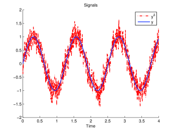
Figure 1: Signal $y$ and noisy signal $y^{\delta}$.

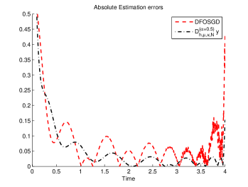
Figure 2: Absolut estimation errors in noise-free case.

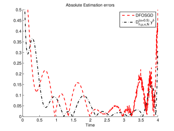
Figure 3: Absolut estimation errors in noisy case.

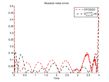
Figure 4: Absolut noise error contributions.

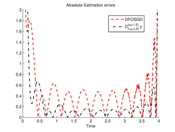
Figure 5: Absolut estimation errors in noise-free case.

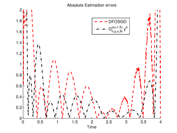
Figure 6: Absolut estimation errors in noisy case.

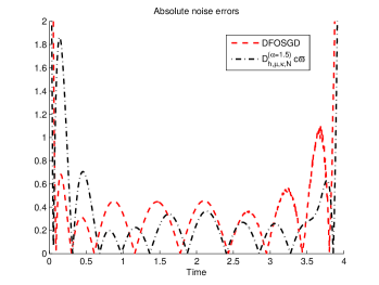
Figure 7: Absolut noise error contributions.

IV CONCLUSION

In this paper, we propose a fractional Jacobi differentiator which is a fractional order differentiator exactly given by an integral formula. This differentiator is deduced from the Jacobi orthogonal polynomial filter and the Riemann-Liouville fractional order derivative definition. It can accurately and easily estimate the fractional order derivatives of noisy signals. There are some parameters $h$, $\mu$, $\kappa$ and $N$ on which the fractional Jacobi differentiator depends. We do not give any analysis on the influence of these parameters on the estimation errors. However, similarly to the integer order differentiation by integration case (see [16, 17, 15, 14]), this study can be easily carried out in a further work. Moreover, we do not use the causal propriety of the fractional Jacobi differentiator in the numerical simulations. It will be used in some interesting applications where the sampling data may be irregularly spaced.

References

- [1] M. Abramowitz and I.A. Stegun, editeurs. Handbook of mathematical functions. GPO, 1965.
- [2] A. Charef, H. H. Sun, Y. Y. Tsao and B. Onaral: Fractal system as represented by singularity function, IEEE Trans. Autom. Control, 37, 9, pp. 1465-1470, 1992.
- [3] D.L. Chen, Y.Q. Chen and D.Y. Xue: Digital Fractional Order Savitzky-Golay Differentiator, IEEE Transactions on Circuits and Systems II: Express Briefs, 58, 11, pp. 758-762, 2011.
- [4] N. Cioranescu: La généralisation de la première formule de la moyenne, Enseign. Math. 37, pp. 292-302, 1938.
- [5] M. Cugnet, J. Sabatier, S. Laruelle, S. Grugeon, B. Sahut, A. Oustaloup and J-M. Tarascon: On Lead-acid battery resistance and cranking capability estimation, IEEE Transactions on Industrial Electronics, 57, 3, pp. 909-917, 2010.
- [6] M. Fliess: Analyse non standard du bruit, C.R. Acad. Sci. Paris Ser. I, 342, pp. 797-802, 2006.
- [7] M. Fliess: Critique du rapport signal à bruit en communications numériques – Questioning the signal to noise ratio in digital communications, International Conference in Honor of Claude Lobry, Revue africaine d’informatique et de Mathématiques appliquées, 9, pp. 419-429, 2008.
- [8] M. Fliess and H. Sira-Ramírez: An algebraic framework for linear identification. ESAIM Control Optim. Calc. Variat., 9, pp. 151-168, 2003.
- [9] M. Fliess, C. Join, M. Mboup and H. Sira-Ramírez: Compression différentielle de transitoires bruités. C.R. Acad. Sci., I(339), pp. 821-826, 2004. Paris.
- [10] M. Fliess, M. Mboup, H. Mounier and H. Sira-Ramírez: Questioning some paradigms of signal processing via concrete examples, in Algebraic Methods in Flatness, Signal Processing and State Estimation, H. Sira-Ramírez, G. Silva-Navarro (Eds.), Editiorial Lagares, México, pp. 1-21, 2003.
- [11] M. Fliess and R. Hotzel: Sur les systèmes linéaires à dérivation non entière. C.R. Acad. Sci. Paris Ser. IIb, (signal, informatique), 324, pp. 99-105, 1997.
- [12] R. Hotzel and M. Fliess: On linear systems with a fractional derivation: Introductory theory with examples. Mathematics and computers in Simulation, 45, pp. 385-395, 1998.
- [13] C. Lanczos: Applied Analysis, Prentice-Hall, Englewood Cliffs, NJ, 1956.
- [14] D.Y. Liu, O. Gibaru and W. Perruquetti: Error analysis for a class of numerical differentiator: application to state observation, 48th IEEE Conference on Decision and Control, Shanghai, China, 2009.
- [15] D.Y. Liu, O. Gibaru and W. Perruquetti: Differentiation by integration with Jacobi polynomials. J. Comput. Appl. Math., 235, 9, pp. 3015-3032, 2011.
- [16] D.Y. Liu, O. Gibaru and W. Perruquetti: Error analysis of Jacobi derivative estimators for noisy signals. Numerical Algorithms, 58, 1, pp. 53-83, 2011.
- [17] D.Y. Liu, O. Gibaru and W. Perruquetti: Convergence Rate of the Causal Jacobi Derivative Estimator. Curves and Surfaces 2011, LNCS 6920 proceedings, pp. 45-55, 2011.
- [18] D.Y. Liu, O. Gibaru, W. Perruquetti, M. Fliess and M. Mboup: An error analysis in the algebraic estimation of a noisy sinusoidal signal. In: 16th Mediterranean conference on Control and automation (MED’08), Ajaccio, France, 2008.
- [19] D.Y. Liu, O. Gibaru and W. Perruquetti: Parameters estimation of a noisy sinusoidal signal with time-varying amplitude. In: 19th Mediterranean conference on Control and automation (MED’11), Corfu, Greece, 2011.
- [20] J.A.T. Machado: Calculation of fractional derivatives of noisy data with genetic algorithms, Nonlinear Dyn., 57, 1/2, pp. 253-260, Jul. 2009.
- [21] M. Mboup: Parameter estimation for signals described by differential equations, Applicable Analysis, 88, pp. 29-52, 2009.
- [22] M. Mboup, C. Join and M. Fliess: A revised look at numerical differentiation with an application to nonlinear feedback control. In: 15th Mediterranean conference on Control and automation (MED’07). Athenes, Greece, 2007.
- [23] M. Mboup, C. Join and M. Fliess: Numerical differentiation with annihilators in noisy environment, Numerical Algorithms 50, 4, pp. 439-467, 2009.
- [24] P. Meer and I. Weiss: Smoothed diferentiation filters for images, J. Visual Comm. Image Repr. 3, pp. 58-72, 1992.
- [25] K.B. Oldham and J. Spanier: The Fractional Calculus, Academic Press, New York 1974.
- [26] A. Oustaloup, B. Mathieu and P. Lanusse: The CRONE control of resonant plants: application to a flexible transmission, European Journal of Control, 1, 2, pp. 113-121, 1995.
- [27] A. Oustaloup, J. Sabatier and X. Moreau: From fractal robustness to the CRONE approach, ESAIM: Proceedings, pp. 177-192, Dec. 1998.
- [28] A. Oustaloup, J. Sabatier and P. Lanusse: From fractal robustness to the CRONE control, FCAA, 1, 2, pp. 1-30, Jan. 1999.
- [29] A. Oustaloup, F. Levron, B. Mathieu and F.M. Nanot: Frequency-band complex noninteger differentiator: Characterization and synthesis, IEEE Trans. Circuits Syst. I, Fundam. Theory Appl., 47, 1, pp. 25-39, 2000.
- [30] P.O. Persson and G. Strang: Smoothing by Savitzky-Golay and Legendre filters, IMA Volume on Math. Systems Theory in Biology, Comm., Comp., and Finance, 134, pp. 301-316, 2003.
- [31] I. Podlubny, Fractional Differential Equations, vol. 198 of Mathematics in Science and Engineering, Academic Press, New York, NY, USA, 1999.
- [32] I. Podlubny, I. Petráš, B.M. Vinagre, P. O’Leary and L. Dorcák: Analogue realizations of fractional-order controllers, Nonlinear Dyn., 29, 1-4, pp. 281-296, Jul. 2002.
- [33] V. Pommier, J. Sabatier, P. Lanusse and A. Oustaloup: CRONE control of a nonlinear hydraulic actuator, Control Engineering Practice, vol. 10, pp. 391-402, Jan. 2002.
- [34] S. Riachy, M. Mboup and J.P. Richard: Multivariate numerical differentiation. J. Comput. Appl. Math., 236, 6, pp. 1069-1089, 2011.
- [35] S. Samadi, M.O. Ahmad and M.N.S. Swamy: Exact fractionalorder differentiators for polynomial signals, IEEE Signal Process. Lett., 11, 6, pp. 529-532, 2004.
- [36] A. Savitzky and M.J.E. Golay: Smoothing and differentiation of data by simplified least squares procedures, Anal. Chem. 36, pp. 1627-1639, 1964.
- [37] R.W. Schafer: What is a Savitzky-Golay filter, IEEE Signal Process. Mag., vol. 28, no. 4, pp. 111-117, Jul. 2011.
- [38] C.C. Tseng and S.L. Lee: Design of fractional order digital differentiator using radial basis function, IEEE Trans. Circuits Syst. I, Reg. Papers, 57, 7, pp. 1708-1718, 2010.
- [39] C.C. Tseng: Improved design of digital fractional-order differentiators using fractional sample delay, IEEE Trans. Circuits Syst. I, Reg. Papers, 53, 1, pp. 193-203, 2006.