Low ionization state plasma in CMEs

Abstract

The Ultraviolet Coronagraph Spectrometer on board the Solar and Heliospheric Observatory (SOHO) often observes low ionization state coronal mass ejection (CME) plasma at ultraviolet wavelengths. The CME plasmas are often detected in O VI (3x10⁵K), C III (8x10⁴K), Ly$\alpha$, and Ly$\beta$, with the low ionization plasma confined to bright filaments or blobs that appear in small segments of the UVCS slit. On the other hand, in situ observations by the Solar Wind Ion Composition Spectrometer (SWICS) on board Advanced Composition Explorer (ACE) have shown mostly high ionization state plasmas in the magnetic clouds in interplanetary coronal mass ejections (ICME) events, while low ionization states are rarely seen. In this analysis, we investigate whether the low ionization state CME plasmas observed by UVCS occupy small enough fractions of the CME to be consistent with the small fraction of ACE ICMEs that show low ionization plasma, or whether the CME plasma must be further ionized after passing the UVCS slit. To do this, we determine the covering factors of low ionization state plasma for 10 CME events. We find that the low ionization state plasmas in CMEs observed by UVCS show average covering factors below 10%. This indicates that the lack of low ionization state ICME plasmas observed by the ACE results from a small probability that the spacecraft passes through a region of low ionization plasma. We also find that the low ionization state plasma covering factors in faster CMEs are smaller than in slower CMEs.

1 Introduction

Coronal mass ejections (CMEs) are among the most explosive solar phenomena. It is important to understand the mechanism of CME eruption and propagation through interplanetary space, which can contribute to understanding the space weather environment. CMEs are often described as a three-part structures: core, cavity, and leading edge (Crifo et al. 1983; Webb 1988). The Ultraviolet Coronagraph Spectrometer (UVCS) on board the Solar and Heliospheric Observatory (SOHO) has observed CME plasmas in UV spectral lines at a few solar radii in corona. The leading edge of CME is often observed in O VI (1032 Å) and Ly$\alpha$ (1216 Å) (e.g. Raymond et al. 2003; Lee et al. 2006) as a diffuse brightening by a modest factor. In contrast, the core of CME is often observed in relatively low formation temperature lines such as C III (977 Å) (Ciaravella et al. 1997, 2000; Lee et al. 2009; Murphy et al. 2011), and it is generally confined to a set of very bright blobs or filaments that appear in small segments of the UVCS slit.

The connection between CMEs and disturbances in the solar wind at 1 AU has been found in the comparison of their plasma characteristics such as temperature and ion composition (see references in Cane & Richardson 2003). For example, CMEs can drive interplanetary shocks (Sheeley et al. 1985). Nowadays, the expanded CME structure and its sheath of swept-up solar wind plasma is referred to as an Interplanetary Coronal Mass Ejection (ICME) (Zhao 1992; Dryer 1994, see also a review for ICME, Howard & Tappin (2009)) The Solar Wind Ion Composition Spectrometer (SWICS) on board Advanced Composition Explorer (ACE) observes ICMEs in situ near Lagrangian point 1, $\sim 1.5$ million km from the Earth toward the Sun. Figure 1 shows ICME and CME material that might be observed by ACE and UVCS, respectively. In CME models, the flux rope may exist before the eruption (Lin & Forbes 2000) or it may form during the eruption (Gosling 1993), but in either case it is believed to evolve into a smoothly rotating magnetic field structure, generally considered to be a flux rope or magnetic cloud in interplanetary space.

Solar wind ionic charge states become “frozen-in” when the ionization and recombination time scales exceed the expansion time scale, i.e. $\tau_{exp}(\equiv\ |\frac{u}{n_{e}}\frac{\partial n_{e}}{\partial r}|^{-1})\ll\tau_{ion}(\equiv\frac{1}{n_{e}(C_{i}+R_{i})})$ (e.g. Hundhausen et al. 1968; Ko et al. 1999), where $u$ is velocity, $n_{e}$ is electron density, $C_{i}$ is ionization rate, and $R_{i}$ is recombination rate. $\tau_{exp}$ and $\tau_{ion}$ are the expansion timescale and ionization/recombination timescale, respectively. A study using an eclipse observation shows that the freezing in height is $\sim$1.5$R_{\sun}$ in the fast solar wind (Habbal et al. 2007). Rakowski et al. (2007) find that the ionization states of Si and Fe freeze in at 2 to 3 $R_{\sun}$ in models of solar eruptions. The lower ionization state ions we consider here, such as H I, C III, and O VI have faster ionization rates and could freeze in at greater heights.

Iron charge state distributions of ICMEs observed by ACE/SWICS show that most magnetic cloud plasmas are highly charged, with ions such as $Fe^{16+}$ (Lepri et al. 2001; Lepri & Zurbuchen 2004). Low ionization states are relatively rare. Lepri & Zurbuchen (2010) show that low ionization state plasmas have been observed only 11 events ($\sim 4\%$ of their events) in a survey of 10 years of SWICS data. In addition, they find that these events originated in filaments near the Sun. UVCS observations have shown that CME plasma is strongly heated even after it leaves the eruption site (Akmal et al. 2001; Lee et al. 2009; Murphy et al. 2011). Comparison of time-dependent ionization models with in situ measurements at 1 AU also requires strong heating in the region around 2$R_{\sun}$ (Rakowski et al. 2007, 2011; Gruesbeck et al. 2011; Lynch et al. 2011). Thus it is possible that the low ionization states observed by UVCS are destroyed as the plasma moves beyond the height of the UVCS slit. It is also possible that much of the low ionization material observed in the corona falls back to the Sun.

Thus the question arises why ACE seldom detects low ionization plasma, while bright, low ionization structures are the salient features of CMEs in UVCS observations. One possibility is that it is a matter of detection criteria. Lepri & Zurbuchen (2010) used stringent selection criteria for low ionization plasma. They used 2 hour binning, and they did not include singly charged ions. Considering that the low ionization states dominate by a large margin in the cool UVCS structures, it is unlikely that ACE would have seen high ionization states but not low if it passed through such a structure. The UVCS structures will expand to several times $10^{11}$ cm by the time they reach 1 AU, so the time resolution is unlikely to be an issue. UVCS generally sees bright C III and O VI, but while C II (1036 Å and 1037 Å) is sometimes observed it has never been found to dominate. Therefore it is unlikely that the exclusion of singly charged ions can account for the difference. We conclude that the low detection rate of low ionization plasma in ICMEs compared with CME observations in the corona is not an artifact of the different measurement techniques. It must therefore is result from a small probability that the spacecraft encounters a clump of low ionization plasma, or else occur because the amount of low ionization plasma at 1 AU is really smaller than the amount at a few solar radii.

In situ observations by the ACE/SWICS represent the plasmas along the ACE trajectory through the ICME (see the left panel of Figure 1). Assuming that the cool plasma maintains the filamentary structure seen by UVCS, the probability that ACE will detect low ionization plasma is proportional to the covering factor of the cool filaments, that is the fraction of the 2D projection of the ICME where cool material is present. Similarly, the UVCS observations of low ionization state plasma at a few solar radii can be transformed into 2D images, and the covering factor of low ionization material equals the probability that a line of sight passes through a low ionization filament or blob (see the right panel of Figure 1). In this analysis, we measure the covering factor of low ionization state plasma observed by SOHO/UVCS. This allows us to determine whether the difference between the low ionization seen by UVCS and the high ionization seen by ACE/SWICS results from a small covering factor of cool plasma, as opposed to heating of CME material as it expands through solar corona or draining of cool plasma back to the Sun.

In §2, we describe the observational data used in this analysis. In §3, we explain how we determine the covering factors of low ionization state CME plasmas observed by UVCS. In §4, we present the covering factors for 10 CME events. In §5, we discuss the results with respect to the heating of CME plasma in lower corona. In addition, we examine an independent list of ICME events for which UVCS observes the corresponding CME plasma to see what fraction shows low ionization material at coronal heights.

2 Observations

SOHO/UVCS (Kohl et al. 1995) observes the solar corona with an instantaneous field of view given by the 40^′ long spectrometer entrance slits as projected on the plane of the sky, which can be placed between 1.5 $R_{\sun}$ and 10 $R_{\sun}$. Different wavelength ranges are covered in different observations because of tradeoffs with spatial and spectral resolution. We select 10 CME events shown in Table 1. These events have been intensively studied for their kinetic and physical properties (see references in Table 2). The UVCS slits are placed between 1.4 $R_{\sun}$ and 2.3 $R_{\sun}$ for these events. The CME speed of the events ranges from about 200 to 2500 $\rm km~{}sec^{-1}$, so both slow and fast CME events are included.

First, we select two particularly well observed events on 2000 June 28 and 2000 Oct. 22 (event numbers 5 and 6 in Table 1). These two events show the shape of erupted prominence material in consecutive UVCS exposures (see §3.1). The observations show very bright emission in the lines C III (977 Å, $8\times 10^{4}$ K) or Ly$\alpha$ (1216 Å, $<7\times 10^{4}$ K in ionization equilibrium) as well as O VI (1032Å, $3\times 10^{5}$ K). The temperatures are formation temperature in ionization equilibrium using CHIANTI 7.0 (Landi et al. 2012). The CME plasma may be far from ionization equilibrium due to its rapid expansion speed, but the low formation temperatures of these ions indicate that the gas was much cooler than coronal temperatures at some point. For both events, the Extreme Ultraviolet Imaging Telescope (EIT) on board SOHO shows a prominence eruption in He II 304 Å on the solar limb.

Second, we select four slow CME events that show speeds of 211$-$498 $\rm km~{}sec^{-1}$ (event numbers 1$-$4 in Table 1). All four events are associated with a prominence eruption (see references in Table 2). However, an eruption on 2000 Feb 11 (event number 4) indicates an $H\alpha$ filament behind the limb as the most likely source (Ciaravella et al. 2003). A few of the four events are associated with B-class X-ray flares (see Table 1).

Lastly, we select four fast CME events that show speeds of 1913$-$2657 $\rm km~{}sec^{-1}$ (event numbers 7$-$10 in Table 1) associated with X-class flares. These events occurred in 2002$-$2003 during solar maximum. EIT 304 Å observations show prominences in the flare occurrence regions associated with these CMEs. However, the observations were taken every 6 hours, and it is not obvious whether the CME events are associated with prominence eruptions or not. The catalog of prominence and filament in the Solar Geophysical Data (SGD) shows a Loop Prominence System (LPS) in 3 cases (see Table 1). The LPSs are observed later than the CME eruption, indicating that the recorded LPS could be a post-flare loop system.

3 Analysis

We measure the covering factors of low ionization state CME plasmas, defined as the fraction of the reconstructed CME image where low ionization material is detected, for 10 CME events observed by SOHO/UVCS. First, we construct two-dimensional images that show CME material along the UVCS slit in consecutive exposures. Then, we calculate the covering factors of low ionization state plasma in an area where CME plasma passes through the UVCS slit in the two-dimensional images. The UVCS observations did not always cover the full extent of the CME, and the events chosen might be biased toward the center of the CME where the prominence material is likely to be seen. Therefore, there is some tendency for the covering factors obtained from the UVCS observations to be larger than would be obtained for the entire CME, but it is probably not a large effect.

3.1 Construction of 2-D image from UVCS observations

In most UVCS CME-watch observations, the UVCS slit is placed at a fixed position over several hours. The observed one-dimensional images of intensity versus position along the slit at a single height can be placed on a 2-D position-time plane with consecutive exposures. This 2-D image represents a temporal scanned image of the event at a fixed position. The time axis can be multiplied by CME speed to obtain an equivalent spatial image. These 2-D images can be found in the LASCO CME catalogue for most of the CME events observed by UVCS.

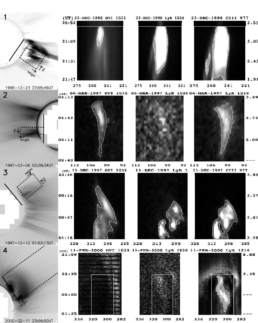
Figure 2: LASCO C2 and UVCS observations. The first left panels show the LASCO observations and the locations of the UVCS slit (solid line). Black dashed lines (box) represent the location of the UVCS 2$-$D image of the right sides estimated by CME velocities in Table 1. Right three panels show the 2$-$D images of OVI, Ly$\alpha$, Ly$\beta$, or CIII. Left axis represents the UVCS observation time. Right axis represents the heights estimated by the CME velocities at the UVCS observation time. The heights of later UVCS observation than LASCO observation are represented as ‘$-$$-$$-$’ which indicates that the material with the mark is not yet erupted on the LASCO observation time shown in the left column. White solid line (box) represents selected area for the covering factor calculation. The events with no white solid line (box) encompasses the entire UVCS 2D image. Contours on 2$-$D images represent selected low ionization CME plasmas.

In Figures 2 to  4, we show the 10 CME events used in this analysis. The first column shows LASCO C2 observations with a solid line segment that represents the position of the UVCS slit for each event. The 2-D images constructed using the observations in O VI, Ly$\alpha$, Ly$\beta$, and CIII are placed in the next panels depending on events. The dotted box in the first column represents the location of the 2-D images on the LASCO observation. The horizontal and the left vertical axes represent polar angles along the slit (counterclockwise from the north pole in degree) and observation time, respectively.

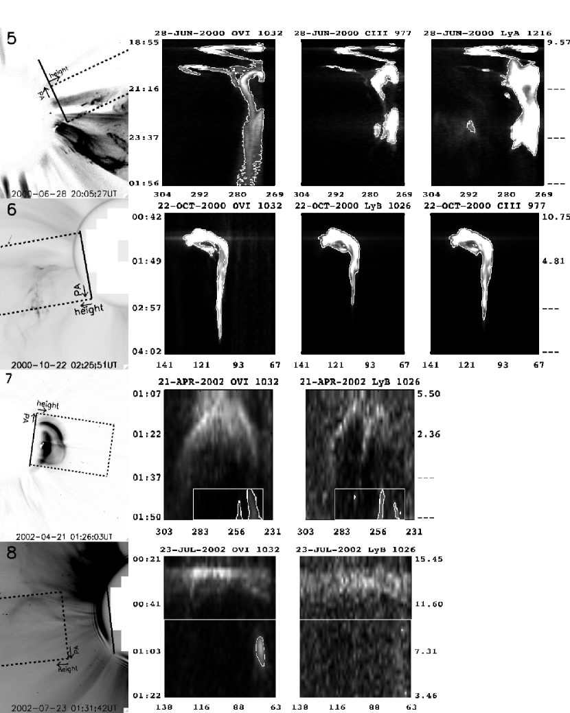
Figure 3: Same as Figure 2 for four more events.

For example, an event on 2000 Oct. 22 helps to understand the constructed 2-D image compared with the LASCO observation (see the second row in Figure 3). The hook shape in the 2D images can be compared with the eruptive prominence on the LASCO observation by rotating of the 2D images 90 ^∘ counterclockwise.

In addition, we show the heights of CME material corresponding to the height at the time observed by UVCS on the 2-D image (the right vertical axis in Figures 2 to 4). The heights are estimated by assuming the constant velocity given in CDAW LASCO CME catalog. However, neither the speed chosen nor the possibility that the CME is not moving perpendicular to the UVCS slit affects the measured covering factor.

3.2 The covering factor of various ionization state CME plasma

We calculate the covering factors of low ionization state CME plasma observed in UV lines, O VI (1032 Å), Ly$\beta$ (1026 Å), C III (977 Å), and Ly$\alpha$ (1216 Å). UVCS often observes low ionization state plasma in the CME core (see a cartoon in the right panel of Figure 1). In this analysis, we exclude the features that indicate CME front and leg because these features are probably ambient coronal plasma with the coronal ionization state. In general the H Lyman lines and O VI lines from the front are diffuse, not very much brighter than the pre-CME corona, and their line widths are at least as large as in the pre-CME observations. On the other hand, prominence material tends to be concentrated in filamentary material, it is very bright, and it often shows a low kinetic temperature based on the narrow line width.

To find the covering factor of the low ionization CME plasma, we first subtract a background. For 9 events, we took the average of 1 to 2 hours of pre-CME exposures as the background. For the event on Dec. 23 1996, the wavelength setting was changed just before the CME occurred, so no background is subtracted. Because the prominence emission in low ionization lines is extremely bright compared to the pre-CME emission, this has little effect on the results. A faint emission feature outside of contour later than 21:10UT in O VI is background emission, so the feature was excluded for selecting the low ionization CME plasmas.

Second, we select the area that does not include the CME front and leg. These are coronal material that is compressed by the expanding flux rope, and while they often appear as enhanced emission regions in Ly$\alpha$ and O VI, the ionization state is that of the ambient corona. For the 1996 Dec. 23, 2002 Jul. 23 and 2003 Nov. 4 events, we use the area below the white line to exclude the background or the CME front. For the 2000 Feb. 11, 2002 Apr. 21 and 2002 Aug. 24 events, we use the area inside the box to exclude the front and leg. For the other events, we take the entire reconstructed UVCS image. We use the same set of spectral lines, O VI, Ly$\beta$, CIII, and Ly$\alpha$ for each event. This allows a comparison of the covering factors for material at different formation temperatures for each event.

Third, we select the low ionization state plasmas (contours in Figures 2 to 4). The contour levels are selected with the lowest value which does not include background noise features. Then the covering factors can be calculated by

$$\mathsf{Covering~{}factor}=\frac{\mathsf{The~{}total~{}number~{}of~{}pixels~{}in~{}contoured~{}area}}{\mathsf{The~{}total~{}number~{}of~{}pixels~{}in~{}selected~{}area}}$$ (1)

The biggest uncertainty in the covering factor comes from the denominator. First, we have chosen the rectangular areas in the UVCS images as large as we can without including emission from the CME front or legs, but the choice is somewhat subjective. It is based upon LASCO movies rather than the images shown the left hand column in Figures 2 to 4, and the images in the figures can be somewhat misleading. In some events, 1996 Dec. 23, 1997 Dec. 12, and 2000 Jun. 28, UVCS observes the partial structures of the CMEs because of the slit location. We exclude the part of the slit outside of the CME structure. Second we give the same weight to each exposure, which is equivalent to assuming a constant speed across the UVCS slit. Acceleration would tend make the areas at later times larger, but in general the expansion speed deep within the CME is smaller than at the front, so the areas at later times would be diminished. These effects probably cause an uncertainty at the 30 to 40% level, which will not affect our conclusion that the covering factor is small.

4 Results

Table 2 shows the covering factors for 10 CME events. A covering factor of 0.00 means that the low ionization line covering factor was smaller than 0.005. Events 1$-$4 are slow CMEs with associated prominence eruptions (see references for each event in Table 2). Event 1 shows several prominence/filament events (ADF, EPL, DSF) near the CME eruption time and location with a small B-class X-ray flare. This event was studied as the first SOHO observation of CME initiation with a prominence eruption (Dere et al. 1997). This event is one of the two events (event 1 and 3) observed in 4 wavelengths (O VI, Ly$\alpha$, Ly$\beta$, and CIII), which allows the comparison of the covering factors for plasma at different formation temperatures. Event 1 shows higher covering factors in Ly$\beta$, CIII, Ly$\alpha$ than in O VI, while in event 3 the O VI covering factor is largest. Event 2 is likely associated with a B8.9 X-ray flare. There is a B-class flare close to the time of event 3. However, the SGD shows the flare without its location information, so it may not be associated with this CME. Event 4 is associated with a prominence eruption behind the limb (Ciaravella et al. 2003).

Events 5 and 6 are associated with prominence eruptions at the solar limb. These events are especially well observed events with cool material. Both events show prominence eruptions in EIT 304 Å observations. Event 5 was observed to exhibit helical motion as the prominence material passed through the UVCS slit (Ciaravella et al. 2005). Event 6 especially shows the hook shape that provides an easy comparison with the LASCO observation (see §3.2). A C-class flare is associated with event 5 while event 6 does not show any associated X-ray flare. These CMEs with speeds of $\sim$1000 $\rm km~{}s^{-1}$ are in the middle of the speed range of the 10 events. The covering factor of C III in event 5 is relatively small compared to O VI and Ly$\alpha$. However, both events show similar covering factors in the different lines.

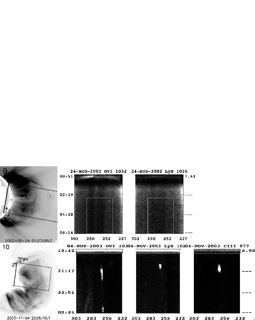
Figure 4: Same as Figure 2 for the final two events.

Events 7 $-$ 10 are fast CMEs ($\gtrsim$2000 $\rm km~{}s^{-1}$). All four events are associated with X-class flares. Event 8 shows ejected material in the LASCO observation that could be the cool material observed in the O VI. Events 7$-$10 are observed in hot spectral lines (Raymond et al. 2003; Ciaravella & Raymond 2008). In the case of event 10, there are ejecta in EIT 195 Å images (Ciaravella & Raymond 2008). UVCS observed small blobs of cool material at three times over the course of many hours, suggesting that those ejecta arose as result of later magnetic field rearrangement (Ciaravella & Raymond 2008). We used a time interval that included only the first cool blob in this analysis (Figure 4), but a similar small covering factor would be obtained with other choices. All the covering factors are small in all 4 fast CME events.

The slow CME events associated with a prominence/filament show relatively larger fractions of cool plasma, while the fast CME events associated with X-class flares show smaller fractions than the slow CME events. This could be because any prominence material in the faster CMEs is more strongly heated, so that it is highly ionized before it reaches the height of the UVCS slit. In addition, the covering factors at the different formation temperatures for each event are mostly similar. Overall, the covering factors in 10 CME events all show small numbers in the range of 0.0$-$0.23. This indicates that the small number of cool ICME events in ACE observations results from a small covering factor of cool plasma.

5 Discussion and Conclusions

We show 26 ICME events in Table 3. The ICMEs are selected for 1996$-$2002 from Cane & Richardson (2003) and for 2003$-$2005 from Richardson & Cane (2010). The list also can be found in their ICME list. The list shows a corresponding CME event for each ICME event. We select the ICME events in which UVCS observes the corresponding CME plasma from LASCO CME catalogue. We exclude cases where the corresponding CME is multiple CMEs or a doubtful association. Two events show a slightly different CME occurrence time in the ICME list and CME catalogue (represented as ^g,h). The events include 3 cool ICME events in Lepri & Zurbuchen (2010) with a mark ^∗.

In Table 3, about half of events are prominence associated. The presence or absence of the associated prominence is indicated in the UVCS pages linked to the LASCO CME catalogue. For a few questionable cases in the catalogue, we examined the UVCS data to determine the presence or absence of cool material. Earlier, it was believed that most CME events are associated with filament/prominence eruption (Webb & Hundhausen 1987). However, a recent study shows many CMEs are detected without low coronal signatures (Ma et al. 2010). The O VI and Ly$\alpha$ can indicate either the front of the CME and a prominence. However, those can be identified by line characteristics (see §3.2). Several events were observed in relatively low temperature lines (e.g. CIII 977 Å ). These are represented with a mark ^∗∗. One event among these four events is associated with a X-class flare, while the other three events are associated with C- and small M- class flares. It is possible that the more energetic flares also have larger heating rates in the ejected prominence region, so that the prominence gas does not appear in low ionization lines in UVCS at coronal heights.

In this analysis, the cool material observed by the UVCS shows a small covering factor, indicating that the small number of cool ICME events detected by ACE results from a small covering factor of cool plasma. Thus there is no evidence that the prominence material must be ionized at heights above the UVCS observations at 1.5$-$2$R_{\sun}$ in order to explain the small fraction of ICMEs that show low ionization material, or that low ionization plasma drains back to the Sun after passing though the heights observed by UVCS. While strong plasma heating is present at these heights (Akmal et al. 2001; Lee et al. 2009; Murphy et al. 2011), the ionization state may be largely frozen-in.

Table 1: CME and Prominence/Filament

event	Date	Timea	Speeda	PAa	Widtha	NOAA	GOES X-ray flareb	Prominence/Filamentb
1	1996 Dec 23	21:16	354	255	58	8005	B2c	ADF  20:06$-$20:11
								EPL  20:11$-$20:48
								DSF  20:16$-$20:46
2	1997 Mar 6	01:36	301	104	27	8020	B8.9  00:41$-$00:52  N02E78d	ASR  00:45$-$10:30
3	1997 Dec 12	01:27	211	291	80		B5.2  00:44$-$01:00	None
4	2000 Feb 11	21:08	498	277	$>$173		None	None
5	2000 Jun 28	19:31	1198	270	$>$134	9046	C3.7  18:48$-$19:10  N20W9	EPL  18:31$-$20:49
6	2000 Oct 22	00:50	1024	103	236		None	EPL  22:30(10/21)$-$01:17
7	2002 Apr 21	01:27	2393	Halo	360	9906	X1.5  00:43$-$02:38  S14W84	LPS  02:01$-$09:56
8	2002 Jul 23	00:42	2285	Halo	360	10039	X4.8  00:18$-$00:47  S13E72	None
9	2002 Aug 24	01:27	1913	Halo	360	10069	X3.1  00:49$-$01:12  S02W81	LPS  01:12$-$07:20
10	2003 Nov 4	19:54	2657	Halo	360	10486	X28   19:29$-$20:06  S19W83	LPS  21:06$-$00:00

Note. — ^a: Time (UT), Linear speed (km/s), PA (deg), and Angular width (deg) in the CME catalog (http://cdaw.gsfc.nasa.gov/CME$\_$list)

^b: Solar Geophysical Data(http://www.ngdc.noaa.gov/stp/solar/sgd.html). ADF: Active Dark Filament, EPL: Eruptive Prominence on the Limb, DSF: Disappearing Solar Filament, ASR: Active Surge Region, LPS: Loop Prominence System

^c: see Dere et al. (1997), No X-ray flare in the Solar Geophysical Data

^d: NOAA active region location

Table 2: Covering factor of low ionization CME plasma

event	Date	PA(deg)a	h(R☉)a	OVI	Ly$\beta$	CIII	Ly$\alpha$	Ref.b
1	1996 Dec 23	235	1.39	0.03	0.18	0.23	0.36	1
2	1997 Mar 6	90	1.55	0.11	0.01	*	0.13	2
3	1997 Dec 12	310	1.63	0.20	0.10	0.16	0.14	3, 4
4	2000 Feb 11	305	2.33	0.00	0.00	*	0.24	5
5	2000 Jun 28	295	2.32	0.15	*	0.08	0.16	6, 7
6	2000 Oct 22	100	1.63	0.06	0.06	0.07	*	7
7	2002 Apr 21	262	1.63	0.14	0.07	*	*	7, 8, 9
8	2002 Jul 23	96	1.63	0.02	0.00	*	*	8, 10, 11
9	2002 Aug 24	260	1.63	0.00	0.00	*	*	8
10	2003 Nov 4	262	1.63	0.01	0.00	0.00	*	12

Note. — *: No UVCS observation in the wavelength ranges

^a: UVCS slit position angle (PA) and height (h)

^b References: 1; Ciaravella et al. (1997), 2; Ciaravella et al. (1999), 3; Ciaravella et al. (2000), 4; Ciaravella et al. (2001), 5; Ciaravella et al. (2003), 6; Ciaravella et al. (2005), 7; Ciaravella et al. (2006), 8; Raymond et al. (2003), 9; Lee et al. (2006), 10; Raymond et al. (2007), 11;Mancuso & Avetta (2008), 12; Ciaravella & Raymond (2008)

Table 3: ICMEs (Cane & Richardson 2003; Richardson & Cane 2010) with UVCS observations

Disturbancea	CMEa	Vel.b	Flarec	PA	h(R☉)d	UVCS obs.	Pe	Notef
1997 02/09 1321	02/07 0030	490	None	270	1.5$-$3.0	OVI	N	L$?$
∗1998 05/01 2156	04/29 1658	1374	M6.8	144	1.9$-$3.8	Ly$\alpha$	Y	V$?$
1998 11/07 0815	11/04 0418g	102	C5.2	359	3.1, 3.6	Ly$\alpha$	N
1999 07/06 1509	07/03 1954	536	C5.6	360	6.1	Ly$\alpha$	N	L
2000 01/22 0023	01/18 1754	739	M3.9	255	1.6, 1.9	Ly$\alpha$, OVI	N	F
2000 02/11 0258	02/08 0930	1079	M1.3	102	2.3, 2.6	Ly$\alpha$	N	F
2000 02/11 2352	02/10 0230	944	C7.3	102, 110	1.9, 2.3	OVI	N	V$?$, L$?$
2000 02/14 0731	02/12 0431	1107	M1	305	2.3	Ly$\alpha$	N	F, V$?$
∗∗2000 04/06 1639	04/04 1632	1188	C9	225	1.4, 1.5	Ly$\alpha$, Ly$\beta$, CIII, OVI, NIII	Y	L
∗2000 07/15 1437	07/14 1054	1674	X5.7	180	1.6$-$4.0	Ly$\alpha$	Y	V$?$
2001 03/03 1121	02/28 1450	313	None	225	3.1, 2.6	OVI	Y	F$?$, L$?$
2001 03/27 1747	03/25 1706	677	C9	360	3.1	Ly$\alpha$	N	F, S$?$
2001 04/04 1455	04/02 2206	2505	X20	223, 225	2.0, 2.5	Ly$\alpha$, OVI	Y	F, S$?$
2001 04/11 1343	04/10 0530	2411	X2.3	270	2.6	Ly$\alpha$	N	F
2001 08/17 1103	08/14 1601	618	None	26	2.0	OVI	Y	F, S$?$
∗∗2001 10/11 1701	10/09 1130	973	M1.4	90$-$180	1.9$-$3.1	Ly$\alpha$, Ly$\beta$, CIII, OVI	Y	F
∗∗2001 11/19 1815	11/17 0530	1379	M2.8	0$-$135	1.7, 1.5	Ly$\alpha$, Ly$\beta$, OVI, SiIII, NIII	Y
2001 11/24 0656	11/22 2330	1437	M9.9	356	2.4	Ly$\alpha$, OVI	Y	F$?$
2002 05/23 1050	05/22 0326h	1557	C5.0	180, 225	1.5$-$1.7	Ly$\alpha$, OVI	Y
∗∗2002 07/17 1603	07/15 2030	1151	X3.0	360	1.7$-$3.6	Ly$\alpha$, Ly$\beta$, CIII, OVI	Y	F, S, V$?$
2003 05/29 1825	05/28 0050	1366	X3.6	360	1.6, 1.7	Ly$\alpha$, OVI	N
∗2003 10/28 0206	10/26 1754	1537	X1.2	245$-$270	1.7$-$3.1	Ly$\alpha$, OVI	N	F, S$?$
2003 10/29 0611	10/28 1130	2459	X17.2	90$-$225	1.7$-$3.1	Ly$\alpha$, OVI	Y	F, S$?$
2003 10/30 1619	10/29 2054	2029	X11	178, 179	2.0, 2.5	Ly$\alpha$, OVI	N	F$?$, L$?$
2005 01/21 1714	01/20 0654	882	X7.1	283	2.3	Ly$\alpha$	N
2005 05/29 0905	05/26 1506	586	B7.5$?$	270	3.0, 2.1	FeXVIII, OVI	N

Note. — ^∗: Cold ICME events in Lepri & Zurbuchen (2010)

^∗∗: Relatively low temperature line observations by UVCS.

^a: The time of associated geomagnetic storm sudden commencement or shock passage in the ICME events and the associated LASCO CME events (Cane & Richardson 2003; Richardson & Cane 2010).

^b: CME speed in the LASCO CME catalog (linear speed km/s)

^c: GOES X-ray flare. It is referred from log files in the CME catalogue and X-ray flare data in SGD. The last one represented with $?$ shows no flare location information in the SGD.

^d: CME plasma detected height. If it is not specified in the catalog, it is the UVCS slit height.

^e: Prominence

^f: L: Leg, F: Front, S: Shock, V: Void

^g: LASCO CME 11/04 0454

^h: LASCO CME 05/22 0350

Figure 1: Left: Low ionization state plasma in ICME observed by ACE, Right: Low ionization state CME plasma observed by UVCS.

References

- Akmal et al. (2001) Akmal, A., Raymond, J. C., Vourlidas, A., Thompson, B., Ciaravella, A., Ko, Y.-K., Uzzo, M., & Wu, R. 2001, ApJ, 553, 922
- Cane & Richardson (2003) Cane, H. V. & Richardson, I. G. 2003, Journal of Geophysical Research (Space Physics), 108, 1156
- Ciaravella & Raymond (2008) Ciaravella, A. & Raymond, J. C. 2008, ApJ, 686, 1372
- Ciaravella et al. (1997) Ciaravella, A., Raymond, J. C., Fineschi, S., Romoli, M., Benna, C., Gardner, L., Giordano, S., Michels, J., O’Neal, R., Antonucci, E., Kohl, J., & Noci, G. 1997, ApJ, 491, L59+
- Ciaravella et al. (2006) Ciaravella, A., Raymond, J. C., & Kahler, S. W. 2006, ApJ, 652, 774
- Ciaravella et al. (2005) Ciaravella, A., Raymond, J. C., Kahler, S. W., Vourlidas, A., & Li, J. 2005, ApJ, 621, 1121
- Ciaravella et al. (2001) Ciaravella, A., Raymond, J. C., Reale, F., Strachan, L., & Peres, G. 2001, ApJ, 557, 351
- Ciaravella et al. (1999) Ciaravella, A., Raymond, J. C., Strachan, L., Thompson, B. J., Cyr, O. C. S., Gardner, L., Modigliani, A., Antonucci, E., Kohl, J., & Noci, G. 1999, ApJ, 510, 1053
- Ciaravella et al. (2000) Ciaravella, A., Raymond, J. C., Thompson, B. J., van Ballegooijen, A., Strachan, L., Li, J., Gardner, L., O’Neal, R., Antonucci, E., Kohl, J., & Noci, G. 2000, ApJ, 529, 575
- Ciaravella et al. (2003) Ciaravella, A., Raymond, J. C., van Ballegooijen, A., Strachan, L., Vourlidas, A., Li, J., Chen, J., & Panasyuk, A. 2003, ApJ, 597, 1118
- Crifo et al. (1983) Crifo, F., Picat, J. P., & Cailloux, M. 1983, Sol. Phys., 83, 143
- Dere et al. (1997) Dere, K. P., Brueckner, G. E., Howard, R. A., Koomen, M. J., Korendyke, C. M., Kreplin, R. W., Michels, D. J., Moses, J. D., Moulton, N. E., Socker, D. G., St. Cyr, O. C., Delaboudinière, J. P., Artzner, G. E., Brunaud, J., Gabriel, A. H., Hochedez, J. F., Millier, F., Song, X. Y., Chauvineau, J. P., Marioge, J. P., Defise, J. M., Jamar, C., Rochus, P., Catura, R. C., Lemen, J. R., Gurman, J. B., Neupert, W., Clette, F., Cugnon, P., van Dessel, E. L., Lamy, P. L., Llebaria, A., Schwenn, R., & Simnett, G. M. 1997, Sol. Phys., 175, 601
- Dryer (1994) Dryer, M. 1994, Space Sci. Rev., 67, 363
- Gosling (1993) Gosling, J. T. 1993, J. Geophys. Res., 98, 18937
- Gruesbeck et al. (2011) Gruesbeck, J. R., Lepri, S. T., Zurbuchen, T. H., & Antiochos, S. K. 2011, ApJ, 730, 103
- Habbal et al. (2007) Habbal, S. R., Morgan, H., Johnson, J., Arndt, M. B., Daw, A., Jaeggli, S., Kuhn, J., & Mickey, D. 2007, ApJ, 663, 598
- Howard & Tappin (2009) Howard, T. A. & Tappin, S. J. 2009, Space Sci. Rev., 147, 31
- Hundhausen et al. (1968) Hundhausen, A. J., Gilbert, H. E., & Bame, S. J. 1968, ApJ, 152, L3+
- Ko et al. (1999) Ko, Y., Gloeckler, G., Cohen, C. M. S., & Galvin, A. B. 1999, J. Geophys. Res., 104, 17005
- Kohl et al. (1995) Kohl, J. L., Esser, R., Gardner, L. D., Habbal, S., Daigneau, P. S., Dennis, E. F., Nystrom, G. U., Panasyuk, A., Raymond, J. C., Smith, P. L., Strachan, L., van Ballegooijen, A. A., Noci, G., Fineschi, S., Romoli, M., Ciaravella, A., Modigliani, A., Huber, M. C. E., Antonucci, E., Benna, C., Giordano, S., Tondello, G., Nicolosi, P., Naletto, G., Pernechele, C., Spadaro, D., Poletto, G., Livi, S., von der Lühe, O., Geiss, J., Timothy, J. G., Gloeckler, G., Allegra, A., Basile, G., Brusa, R., Wood, B., Siegmund, O. H. W., Fowler, W., Fisher, R., & Jhabvala, M. 1995, Sol. Phys., 162, 313
- Landi et al. (2012) Landi, E., Del Zanna, G., Young, P. R., Dere, K. P., & Mason, H. E. 2012, ApJ, 744, 99
- Lee et al. (2006) Lee, J., Raymond, J. C., Ko, Y., & Kim, K. 2006, ApJ, 651, 566
- Lee et al. (2009) —. 2009, ApJ, 692, 1271
- Lepri & Zurbuchen (2004) Lepri, S. T. & Zurbuchen, T. H. 2004, Journal of Geophysical Research (Space Physics), 109, 1112
- Lepri & Zurbuchen (2010) —. 2010, ApJ, 723, L22
- Lepri et al. (2001) Lepri, S. T., Zurbuchen, T. H., Fisk, L. A., Richardson, I. G., Cane, H. V., & Gloeckler, G. 2001, J. Geophys. Res., 106, 29231
- Lin & Forbes (2000) Lin, J. & Forbes, T. G. 2000, J. Geophys. Res., 105, 2375
- Lynch et al. (2011) Lynch, B. J., Reinard, A. A., Mulligan, T., Reeves, K. K., Rakowski, C. E., Allred, J. C., Li, Y., Laming, J. M., MacNeice, P. J., & Linker, J. A. 2011, ApJ, 740, 112
- Ma et al. (2010) Ma, S., Attrill, G. D. R., Golub, L., & Lin, J. 2010, ApJ, 722, 289
- Mancuso & Avetta (2008) Mancuso, S. & Avetta, D. 2008, ApJ, 677, 683
- Murphy et al. (2011) Murphy, N. A., Raymond, J. C., & Korreck, K. E. 2011, ArXiv e-prints
- Rakowski et al. (2007) Rakowski, C. E., Laming, J. M., & Lepri, S. T. 2007, ApJ, 667, 602
- Rakowski et al. (2011) Rakowski, C. E., Laming, J. M., & Lyutikov, M. 2011, ApJ, 730, 30
- Raymond et al. (2003) Raymond, J. C., Ciaravella, A., Dobrzycka, D., Strachan, L., Ko, Y., Uzzo, M., & Raouafi, N. 2003, ApJ, 597, 1106
- Raymond et al. (2007) Raymond, J. C., Holman, G., Ciaravella, A., Panasyuk, A., Ko, Y., & Kohl, J. 2007, ApJ, 659, 750
- Richardson & Cane (2010) Richardson, I. G. & Cane, H. V. 2010, Sol. Phys., 264, 189
- Sheeley et al. (1985) Sheeley, Jr., N. R., Howard, R. A., Michels, D. J., Koomen, M. J., Schwenn, R., Muehlhaeuser, K. H., & Rosenbauer, H. 1985, J. Geophys. Res., 90, 163
- Webb (1988) Webb, D. F. 1988, J. Geophys. Res., 93, 1749
- Webb & Hundhausen (1987) Webb, D. F. & Hundhausen, A. J. 1987, Sol. Phys., 108, 383
- Zhao (1992) Zhao, X. 1992, J. Geophys. Res., 97, 15051