Sigma meson and lowest possible glueball candidate in an extended linear $\sigma$ model

Abstract

We formulate an extended linear $\sigma$ model of a quarkonia nonet and a tetraquark nonet as well as a complex iso-singlet (glueball) field to study the low-lying scalar meson. Chiral symmetry and $U_{A}(1)$ symmetry and their breaking play important role to shape the scalar meson spectrum in our work. Based on our study we will comment on what may be the mass of the lowest possible scalar and pseudoscalar glueball states. We will also discuss on what may be the nature of the sigma or $f_{0}(600)$ meson.

1 Introduction

Theoretical understanding of the so-called Higgs Boson of QCD namely the $\sigma$ or $f_{0}(600)$ meson is important as they play an important role in chiral symmetry breaking and can be used as a probe for QCD vacuum. While the confirmation of its existence from $\pi\pi$ scattering process puts an end to the decades-long controversy Caprini:2005zr ; Scalar , the agreement on the nature of $\sigma/f_{0}(600)$ however has not yet been achieved. The tetraquark model jaffe supports $\sigma/f_{0}(600)$ to be a tetraquark state. Whereas, recent data from $\pi\pi$ and $\gamma\gamma$ scattering Minkowski:1998mf ; arXiv:0804.4452 suggest it has a sizable fraction of glueball and another study from K-matrix analysis Mennessier:2010xg suggested that $f_{0}(600)/\sigma$ should be a glueball dominant state.

On the other hand the agreement on the lowest possible iso-scalar and pseudoscalar glueball states has neither been acheived. The result from Lattice simulations suggests $f_{0}(1500)$ or $f_{0}(1700)$ could be a glueball rich iso-scalar, while $\eta(1489)$ can be a glueball rich pseudoscalar Mathieu:2008me .

The great success of chiral symmetry in understanding the nature of lightest pseudo-scalars motivates us to use an extended version of linear $\sigma$ models qishu ; Fariborz:2011es to study the nature of these low-lying isoscalars and pseudoscalars. The motivation for constructing an extended linear sigma model consisting of effective quarkonia, tetraquark and glueball fields comes from the physical considerations that scalar condensates are allowed by the QCD vacuum. So in principle apart from quarkonia and tetraquark condensates, scalar glueball condensate should also be present in the QCD vacuum and need to be considered while studying the vacuum excitation. The mixing pattern followed in our framework comes from the consideration that mesons having identical external quantum numbers can mix even if they have different internal flavour structures. Based on these premises we attempt to study the nature of $\sigma/f_{0}(600)$ meson as well as lowest iso-scalar and pseudoscalar glueball candidate. In the following section we briefly review the model Lagrangian and the symmetry breaking pattern. At last we will present our results and conclude.

2 Model

The extended linear $\sigma$ model can be systematically formulated under the symmetry group $SU_{R}(3)\times SU_{L}(3)\times U_{A}(1)$. Three types of chiral fields are included: a $3\times 3$ matrix field $\Phi$ which denotes the quarkonia states, a $3\times 3$ matrix field $\Phi^{\prime}$ which denotes the tetraquark state, and a complex chiral singlet field $Y$ which denotes the pure glueball states.

Up to the mass dimension $O(p^{4})$ (we assume that they are the most important operators to determine the nature of light scalars of ground states), the Lagrangian of our model can include two parts: the symmetry invariant part ${\cal L}_{S}$ and the symmetry breaking one ${\cal L}_{SB}$. The symmetry invariant part includes those terms which respect $SU(3)_{L}\times SU(3)_{R}$ symmetry as well as $U_{A}(1)$ symmetry:

$${\cal L}_{S} =Tr(\partial_{\mu}\Phi\partial^{\mu}\Phi^{\dagger})+Tr(\partial_{\mu}\Phi^{\prime}\partial^{\mu}\Phi^{\dagger\prime})+\partial_{\mu}Y\partial^{\mu}Y^{\star}-{m_{\Phi}}^{2}Tr(\Phi^{\dagger}\Phi)-{m_{\Phi^{\prime}}}^{2}Tr(\Phi^{\dagger\prime}\Phi^{\prime})$$ (1)

$$-{m_{Y}}^{2}YY^{\star}-\lambda_{1}Tr(\Phi^{\dagger}\Phi\Phi^{\dagger}\Phi)-{\lambda_{1}}^{\prime}Tr(\Phi^{\dagger\prime}\Phi^{\prime}\Phi^{\dagger\prime}\Phi^{\prime})-\lambda_{2}Tr(\Phi^{\dagger}\Phi\Phi^{\dagger\prime}\Phi^{\prime})-\lambda_{Y}(YY^{\star})^{2}$$

$$-[\lambda_{3}\epsilon_{abc}\epsilon^{def}{\Phi_{d}}^{a}{\Phi_{e}}^{b}{\Phi_{f}}^{\prime c}+h.c.]+[k\,\,YDet(\Phi)+h.c.],$$

While the symmetry breaking part includes the following terms

$${\cal L}_{SB}=[Tr(B.\Phi)+h.c.]+[Tr(B^{\prime}.\Phi^{\prime})+h.c.]+(D.Y+h.c.)-[\lambda_{m}Tr(\Phi\Phi^{\dagger\prime})+h.c.].$$ (2)

To construct the symmetric terms in the Lagrangian we closely follow fariborz1 where the choice of terms are limited by the number of internal quark plus antiquark lines at the effective vertex, which is set to 8. This condition is relaxed for two terms with coupling constants ${\lambda_{1}}^{\prime}$ and $\lambda_{2}$ and the reason to include these two terms stems from the practical consideration of making sure our potential is bounded. For detailed discussion on the terms appearing in the Lagrangian please refer to OurPaper . As evident from the Lagrangian both chiral symmetry $SU(3)_{L}\times SU(3)_{R}$ and $U(1)_{A}$ symmetry are explicitly broken by the terms in ${\cal L}_{SB}$. The $3\times 3$ matrices $B$ and $B^{\prime}$ responsible for the breaking of the symmetry can be parametrized as: $B(B^{\prime})=T_{a}b_{a}(T_{a}{b_{a}}^{\prime})$ ($T_{a}$ are the generators of $U(3)$ with $T_{0}=\sqrt{\frac{1}{6}}{\rm 1\rule{0.43057pt}{6.54443pt}\hskip 0.86108pt}$).

Since the vacuum expectation values of the quarkonia and tetraquark fields can carry those quantum numbers which are allowed by the QCD vacuum, only $a=(0,3,8)$ fields are allowed. The choice of this external fields $b_{a}({b_{a}}^{\prime})$ control the nature and extent of the symmetry breaking. Out of various possible symmetry breaking scenarios, we consider the following case in our present study where:

• $b_{0}({b_{0}}^{\prime})\neq 0$, $b_{3}({b_{3}}^{\prime})=0$ and $b_{8}({b_{8}}^{\prime})\neq 0$. In this case, $U(3)_{A}$ and $SU(3)_{V}$ both are explicitly broken and $SU(3)_{V}$ is broken to $SU(2)_{V}$. As a result $m_{u}=m_{d}\neq m_{s}$, where $m_{i}$ is the quark mass of the $i^{th}$ flavour.

This is reasonable considering the up and down quark masses are nearly equal to each other and thereby indicating $SU(2)_{V}$ is a good (approximate) symmetry. The remnant $SU(2)_{V}$ isospin symmetry allows us to represent two condensates for quarkonia and teraquark fields each as: $v_{0}$, $v_{8}$ and ${v^{\prime}}_{0}$, ${v^{\prime}}_{8}$ respectively. While the gluonic condensate in our theory is labeled as $v_{y}$.

3 Results and Conclusion

Due to the unbroken $SU_{V}(2)$ isospin symmetry, physical scalar and pseudo-scalar states can be categorized into three groups with isospin quantum numbers as $I=1$ (triplet), $\frac{1}{2}$ (doublet) and $0$, respectively. Only bare quarkonia, tetraquark and glueball fields with the same isospin quantum number can mix with each other to form physical states. Moreover, there is no mixing between scalar and pseudoscalar fields. Thus the chiral singlet glueball field can only mix with the isospin singlets of quarkonia and tetraquark fields. Using these facts, the physical states below 2 GeV can be tabulated as given in Table 1, where the isodoublet $\{K,K^{\prime}\}$ is connected with the isodoublet {$K^{*},K^{*\prime}$} by charge conjugation. And a similar relation holds for $\{\kappa$, $\kappa^{\prime}\}$ and $\{\kappa^{*}$, $\kappa^{*\prime}\}$.

Isospin	$I=1$	$I=\frac{1}{2}$	$I=0$
PseudoScalars(P=-1)	$\{\pi,\pi^{\prime}\}$	{K, $K^{\prime}$}, {$K^{*},K^{*\prime}$}	{$\eta_{1},\eta_{2},\eta_{3},\eta_{4},\eta_{5}$ }
Scalars(P=1)	{$a$, $a^{\prime}$ },	{$\kappa$, $\kappa^{\prime}$}, {$\kappa^{*}$, $\kappa^{*\prime}$},	$\{f_{1},f_{2},f_{3},f_{4},f_{5}\}$

Table 1: The categorization of scalar and pseudo-scalar states in term of isospin quantum number are demonstrated. States in the same category can mix with each other.

There are 15 parameters in our model. To solve these parameters we treat the tetraquark vacuum condensates as well as the mixing angles for isotriplet ($\theta_{\pi}$) and isodoublet ($\theta_{K}$) fields as input parameters. Then from the mass matrices of $a,a^{\prime}$, $\kappa$ and $\kappa^{\prime}$, parameters related to isotriplet and isodublet sectors are solved. The symmetry parameters $\{b_{0},b_{8},b_{0}^{\prime},b_{8}^{\prime},D\}$ are solved from the vacuum stability conditions. Whereas, to solve for the parameters related to glueball sector, we use following two conditions:

$$Tr[{M_{\eta}}^{2}]_{Model}=Tr[{M_{\eta}}^{2}]_{Exp}\,\,,\hskip 36.135ptDet[{M_{\eta}}^{2}]_{Model}=Det[{M_{\eta}}^{2}]_{Exp}\,\,.$$ (3)

At the end we are left with one free parameter which is bare glueball mass $m_{Y}$ and is used in our study as a scanning parameter.

For space constriant we refer to OurPaper for details on parameter fixing and method to choose the best fit solution. In choosing the best fit solution we vary the $\pi^{\prime}$ mass from $1.2-1.4$ GeV and choose those solution which give the tree level decay width for $f_{0}(600)\rightarrow\pi\pi$ between $0.35-0.9$ GeV.

Our best fit parameter set is presented in Table (2). We would like to highlight a few features out from it. 1) In absence of the explicit symmetry breaking terms, it is the negative mass parameter ${m_{\Phi}}^{2}$ that would trigger the spontaneous chiral symmetry breaking. 2) The sign of $v_{Y}$ is correlated with the sign of $k$, and the sign of $k$ is determined from the mass spectra of pseudoscalar sector. 3) The couplings $\lambda_{1}$, $\lambda_{1}^{\prime}$, $\lambda_{Y}$ are positive which guarantee the potential is bounded from below. 4) The values of $\lambda_{1}$, $\lambda_{2}$, and $\lambda_{Y}$ as well as $k$ are large, which demonstrate the non-perturbative nature of the model.

  

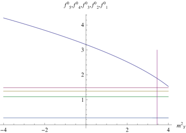
Figure 1: (Left figure) The dependence of $\lambda_{Y}$ upon $m_{Y}^{2}$ is demonstrated. A solid circle marker shows the point $\lambda_{Y}=0$, which corresponds to $m_{Y}^{2}=3.452$ ($m_{Y}=1.858$) . (Right figure) The dependence of mass of $f_{0}$ upon $m_{Y}^{2}$ is demonstrated. A vertical line with $m_{Y}^{2}$ is drawn to read out the lowest mass $m_{f_{0}^{5}}=1.86$.

Parameter	Value	Parameter	Value	Parameter	Value
$\theta_{\pi}$ (radian)	-0.604	${\lambda_{1}}^{\prime}$	8.248	${m_{\Phi}}^{2}$ ($GeV^{2}$)	-0.025
$\theta_{K}$ (radian)	-0.714	$\lambda_{2}$	76.428	${b_{0}}^{\prime}$ ($GeV^{3}$)	0.166
$v_{0}$ (GeV)	0.074	$\lambda_{3}$ (GeV)	-0.738	${m_{\Phi^{\prime}}}^{2}$ ($GeV^{2}$)	0.744
$v_{8}$ (GeV)	-0.115	$\lambda_{Y}$	38.327	${b_{8}}^{\prime}$ ($GeV^{3}$)	0.18
${v_{0}}^{\prime}$ (GeV)	0.203	k	-78.15	$\lambda_{1}$	35.465
${v_{8}}^{\prime}$ (GeV)	0.126	$\lambda_{m}$ ($GeV^{2}$)	-1.044	D ($GeV^{3}$)	-0.265
$v_{y}$ (GeV)	-0.109	$b_{0}$ ($GeV^{3}$)	-0.085
${m_{Y}}^{2}$ ($GeV^{2}$)	3.0	$b_{8}$ ($GeV^{3}$)	-0.161

Table 2: The values of parameters in our fit are shown where the best value of $m_{\pi{{}^{\prime}}}$ is found to be $m_{\pi^{\prime}}=1.2$ GeV.

Meson	Our Value (GeV)	quarkonia ($\%$)	tetraquark ($\%$)	glueball ($\%$)	Experimental Value (GeV)
$\eta_{5}$	1.858	0.037	0.001	99.962	1.756 $\pm$ 0.009
$\eta_{4}$	1.380	75.803	24.167	0.03	1.476 $\pm$ 0.004
$\eta_{3}$	1.291	26.700	73.294	0.006	1.294 $\pm$ 0.004
$\eta_{2}$	0.907	15.852	84.145	0.003	0.958 $\pm$ $24\times 10^{-5}$
$\eta_{1}$	0.595	81.607	18.393	0.0	0.548 $\pm$ $24\times 10^{-6}$
${f_{5}}^{0}$	2.09	0.01	0.0	99.99	-
${f_{4}}^{0}$	1.487	77.469	22.53	0.001	1.505 $\pm$ 0.006
${f_{3}}^{0}$	1.347	22.177	77.82	0.003	1.2-1.5
${f_{2}}^{0}$	1.124	21.561	78.439	0.0	0.980 $\pm$ 0.010
${f_{1}}^{0}$	0.274	78.784	21.211	0.005	0.4-1.2

Table 3: Mass spectra and components for the pseudo-scalar amd scalar mesons based on our fit are shown where the best value of $m_{\pi{{}^{\prime}}}$ is found to be $m_{\pi^{\prime}}=1.2$ GeV.

It is found that the condition $\lambda_{Y}>0$ can predict the lightest glueball scalar should be around 2.0 GeV or so, as can be read off from Fig. (1b), while the lightest glueball pseudo scalar should be $\eta_{5}$. The mass splitting between these two glueball states is controlled by parameters $v_{Y}$ and $\lambda_{Y}$ and is found to be around $0.15$ GeV. When compared with the Lattice QCD prediction for the glueball bare mass reported in lattice where the mass is $1.611$ GeV, our result $m_{Y}=1.73$ GeV is slightly heavier than this prediction. When $m_{Y}=1.611$ GeV is taken, then the predicted mass of the lightest glueball is $m_{f_{5}^{0}}=2.29$ GeV. 3) The lightest scalar $f_{1}^{0}(600)$ is found to be $0.27$ GeV or so and is a quarkonia dominant state.

In Figure 1, we demonstrate the dependence of $\lambda_{Y}$ and $f^{0}$ masses upon the free parameter $m_{Y}^{2}$ with the rest of parameters are given in Table (2). As shown in Fig. (1a), when $m_{Y}^{2}$ is larger than $3.4$ GeV², the $\lambda_{Y}$ becomes negative. Then the potential of our model has to confront with the problem of unbounded vacuum from below. In the allowed values of $m_{Y}^{2}$, the masses of $f^{0}_{i}\,,i=1,2,3,4$ are almost independent of its value, as demonstrated in Fig. (1b). The upper bound of $m_{Y}^{2}$ is determined from the condition $\Gamma_{f^{0}_{1}}>0.35$ GeV.

To conclude, our model predicts that the isoscalar glueball should be heavier than $2.0$ GeV when the pseudoscalar $\eta(1726)$ is the best glueball candidates. The lowest isoscalar $f_{0}(600)$ is found to be quarkonia dominant state with a considerable tetraquark component.

References

- (1) I. Caprini, G. Colangelo and H. Leutwyler, Phys. Rev. Lett. 96, 132001 (2006) [hep-ph/0512364].
- (2) K. F. Liu, arXiv:0805.3364 [hep-lat]; K. F. Liu and C. W. Wong, Phys. Lett. B 107, 391 (1981); H. Y. Cheng, C. K. Chua and K. F. Liu, Phys. Rev. D 74, 094005 (2006); Q. Zhao, B. s. Zou and Z. b. Ma, Phys. Lett. B 631, 22 (2005); D. V. Bugg, M. J. Peardon and B. S. Zou, Phys. Lett. B 486, 49 (2000).
- (3) R. L Jaffe, Phys. Rev. D15, 267, 1977.
- (4) P. Minkowski and W. Ochs, Eur. Phys. J. C 9, 283 (1999) [hep-ph/9811518].
- (5) G. Mennessier, S. Narison and W. Ochs, Phys. Lett. B 665, 205 (2008) [arXiv:0804.4452 [hep-ph]].
- (6) G. Mennessier, S. Narison and X. G. Wang, Phys. Lett. B 688, 59 (2010) [arXiv:1002.1402 [hep-ph]].
- (7) V. Mathieu, N. Kochelev and V. Vento, Int. J. Mod. Phys. E 18, 1 (2009) [arXiv:0810.4453 [hep-ph]].
- (8) S. He, M. Huang and Q. S. Yan, Phys. Rev. D 81, 014003 (2010).
- (9) A. H. Fariborz, arXiv:1109.2630 [hep-ph].
- (10) A. H. Fariborz, R. Jora, J. Schechter, Phys. Rev. D 76, 014011 (2007).
- (11) T K Mukherjee, M. Huang and Q. S. Yan, arXiv:1203.5717.
- (12) C. Michael, Hadron 97 Conference, AIP Conf. Proc. 432 (1998) 657.