Probing quantum coherence in qubit arrays

Abstract

We discuss how the observation of population localization effects in periodically driven systems can be used to quantify the presence of quantum coherence in interacting qubit arrays. Essential for our proposal is the fact that these localization effects persist beyond tight-binding Hamiltonian models. This result is of special practical relevance in those situations where direct system probing using tomographic schemes becomes infeasible beyond a very small number of qubits. As a proof of principle, we study analytically a Hamiltonian system consisting of a chain of superconducting flux qubits under the effect of a periodic driving. We provide extensive numerical support of our results in the simple case of a two-qubits chain. For this system we also study the robustness of the scheme against different types of noise and disorder. We show that localization effects underpinned by quantum coherent interactions should be observable within realistic parameter regimes in chains with a larger number of qubits.

I Introduction

Transport processes are of fundamental importance in a wide variety of physical and biological systems, ranging from the actual motion of particles on a lattice [1, 2] to the transfer of classical and quantum information across spin or harmonic chains [3, 4, 5]. Relevant for our purposes, there exist specific features of the transport process that are intrinsically linked to the dynamics of the chain and in particular to whether or not the chain elements can interact coherently [6]. In the mid-$80$’s the motion of a charged particle on a one-dimensional lattice under the influence of a time-dependent electric field was studied and shown to exhibit dynamic localization (DL) [1]. The canonical situation to illustrate this phenomenon is provided by an infinite linear chain of sites along which a charged particle moves under the combined influence of a nearest-neighbour exchange interaction and a time-dependent external driving. In that setting, it was found that the mean-square displacement of the particle as a function of the field modulation $E_{1}$, rather than exhibiting a diffusive behaviour, does not grow without bounds but oscillates sinusoidally. A related phenomenon is the so called coherent destruction of tunneling (CDT), initially formulated in dissipationless conditions for a symmetric, externally driven, double-well potential [7] and subsequently also studied in a dissipative environment [8] (and references therein). Both DL and CDT are genuine manifestations of coherent quantum effects resulting from the interference between different transition paths that leads to the selective inhibition of transport [9]. In contrast, in the classical case, and from an initially localized state, an equilibrium state would be attained in which neighbouring sites would be equally populated.
Ample experimental evidence supports the existence of both types of localization effects in a variety of systems. DL has been observed in Rydberg atoms, where the localization regime is characterized by a ”freezing” of the width of the wave packet with respect to the Rydberg levels [10]; in driven quantum wells or semiconductor superlattices, where a suppression of the conductance was observed [11]; in ultracold atoms interacting with a standing wave of near-resonant light, where this phenomenon was found in the suppression of momentum [12, 13]. There exist also experimental proposals to use CDT as a means to control the dynamics of ultracold atoms in optical lattices [14] and to create long-distance entanglement between atoms with the possibility to use it in the implementation of quantum logical gates [14, 15]. CDT has also been recently observed in both noninteracting [16] and interacting systems [17]. Further, motivated by the desire to study the effects of quantum coherence and dephasing noise and the interplay of the two on transport processes in biological systems [18], recently the detection of dynamic localization was proposed as a way to demonstrate the possible existence of coherence effects in ion channels [19], i.e. protein complexes that regulate the flow of particular ions across the cell membrane and that are essential for a wide variety of cellular functions.

Here we extend this work and discuss the possibility of observing localization effects beyond the canonical setting, including deviations from a strict tight-binding Hamiltonian as well as the inclusion of non-Hamiltonian (noisy) effects. We will show that signatures of localization effects can still be observed in this case and apply these results to the problem of qualitatively witnessing quantum coherence in an interacting chain of superconducting qubits.

II Renormalization of intra-qubit interactions by means of an external modulation

Motivated by specific qubit realizations in the solid state, we analyze an array of interacting qubits subject to a Hamiltonian of the form ($\hbar=1$):

$$H_{0}=\sum_{k=1}^{N}\frac{\omega_{k}}{2}\sigma_{k}^{z}+\sum_{k=1}^{N-1}J_{k,k+1}\sigma_{k}^{x}\sigma_{k+1}^{x},$$ (1)

with $N$ denoting the number of qubits in the chain, $\omega_{k}$ the site energies for each qubit, and $J_{k,k+1}$ the coupling between neighbouring qubits $k$ and $k+1$. In the presence of a time-dependent external driving of the form

$$H_{\rm ac}(t)=\frac{1}{2}\sum_{k=1}^{N}k\cdot E_{\rm ac}\cos(\omega t)\sigma_{k}^{z}$$ (2)

the Hamiltonian $H(t)=H_{0}+H_{\rm ac}(t)$ of the chain reads

$$H=\frac{1}{2}\sum_{k=1}^{N}\big{(}\omega_{k}+kE_{\rm ac}\cos(\omega t)\big{)}\sigma_{k}^{z}+\sum_{k=1}^{N-1}J_{k,k+1}\sigma_{k}^{x}\sigma_{k+1}^{x}.$$ (3)

With the substitution $\sigma_{k}^{x}=\sigma_{k}^{+}+\sigma_{k}^{-}$, the Hamiltonian above can be rewritten as the sum of three contributions,

$$H(t)=H_{z}(t)+H_{1}+H_{2}$$ (4)

with,

$$H_{z}(t)\equiv\frac{1}{2}\sum_{k=1}^{N}\big{(}\omega_{k}+kE_{\rm ac}\cos(\omega t)\big{)}\sigma_{k}^{z}$$ (5)

$$H_{1}\equiv\sum_{k=1}^{N-1}J_{k,k+1}\big{(}\sigma^{+}_{k}\sigma^{-}_{k+1}+\textrm{h.c.}\big{)}$$ (6)

$$H_{2}\equiv\sum_{k=1}^{N-1}J_{k,k+1}\big{(}\sigma^{+}_{k}\sigma^{+}_{k+1}+\textrm{h.c.}\big{)}.$$ (7)

Defining the total excitation number operator as

$$\hat{N}\equiv\sum_{k=1}^{N}\sigma_{k}^{+}\sigma_{k}^{-}$$ (8)

it is easy to see that $[H_{z}(t),\hat{N}]=[H_{1},\hat{N}]=0$ while $[H_{2},\hat{N}]\neq 0$. For this reason, the term $H_{1}$ is usually referred to as an exchange interaction, in the sense that it allows for a hopping of the excitations within the chain, but it does not create nor annihilate them. This is the canonical interaction in previous studies of dynamical localization in systems that can be modelled with a tight-binding Hamiltonian [1].

In the following lines we will show that the interactions described by the terms $H_{1}$ and $H_{2}$ can be indeed enhanced or inhibited separately by the proper tuning of frequency $\omega$ and amplitude $E_{\rm ac}$ of the external field.
To gain insight into the problem, it is convenient to move to an interaction picture with respect the time-dependent term $H_{z}(t)$. That is, we first define

$$U_{0}(t)\equiv\exp_{+}\left\{-i\int_{0}^{t}d\tau H_{z}(\tau)\right\}=\exp\left\{-i\int_{0}^{t}d\tau H_{z}(\tau)\right\}$$ (9)

where we have made use that $H_{z}(t)$ commutes with itself at different times to write the last equality above. Computing explicitly the integral above and taking into account that the operators acting on different sites commute, we have that

$$U_{0}=\prod_{k=1}^{N}\exp\left\{-i\frac{\omega_{k}t}{2}\sigma_{k}^{z}-i\frac{kE_{\rm ac}}{2\omega}\sin(\omega t)\sigma_{k}^{z}\right\}$$ (10)

Hence, the interaction picture Hamiltonian of our chain can be written as

$$H^{\prime}(t)\equiv U_{0}(t)^{\dagger}(H_{1}+H_{2})U_{0}(t)\equiv H^{\prime}_{1}(t)+H^{\prime}_{2}(t),$$ (11)

where we have defined $H^{\prime}_{1}(t)\equiv U_{0}(t)^{\dagger}H_{1}U_{0}(t)$ and $H^{\prime}_{2}(t)\equiv U_{0}(t)^{\dagger}H_{2}U_{0}(t)$. Now, making use of eq. (10) and the Jacobi-Anger expansion $e^{iz\sin(\phi)}=\sum_{n=-\infty}^{\infty}J_{n}(z)e^{in\phi}$, where $J_{n}(x)$ are the Bessel functions of first kind, we can proceed further and evaluate the form of these terms explicitly as:

$$H^{\prime}_{1}(t)=\sum_{k=1}^{N-1}J_{k,k+1}\sigma^{+}_{k}\sigma^{-}_{k}\exp\left\{i(\omega_{k}-\omega_{k+1})t-i\frac{E_{\rm ac}}{\omega}\sin(\omega t)\right\}+\textrm{h.c.}$$ (12)

$$=\sum_{k=1}^{N-1}J_{k,k+1}\sigma^{+}_{k}\sigma^{-}_{k}e^{i(\omega_{k}-\omega_{k+1})t}\sum_{n=-\infty}^{\infty}J_{n}\left(\frac{E_{\rm ac}}{\omega}\right)e^{inwt}+\textrm{h.c.}$$

$$H^{\prime}_{2}(t)=\sum_{k=1}^{N-1}J_{k,k+1}\sigma^{+}_{k}\sigma^{+}_{k}\exp\left\{i(\omega_{k}+\omega_{k+1})t+i\frac{E_{\rm ac}(2k+1)}{\omega}\sin(\omega t)\right\}+\textrm{h.c.}$$ (13)

$$=\sum_{k=1}^{N-1}J_{k,k+1}\sigma^{+}_{k}\sigma^{+}_{k}e^{i(\omega_{k}+\omega_{k+1})t}\sum_{n=-\infty}^{\infty}J_{n}\left(\frac{E_{\rm ac}(2k+1)}{\omega}\right)e^{inwt}+\textrm{h.c.}$$

For the sake of clarity we will consider in the following the case of a homogeneous chain with $\omega_{k}=\omega_{0}$ and $J_{k,k+1}=J$ for all values of $k$. Under this assumption the Hamiltonian $H^{\prime}(t)$ can be written as:

$$H^{\prime}(t)=\sum_{k=1}^{N-1}g(t)\sigma_{k}^{+}\sigma_{k+1}^{-}+g^{\prime}_{k}(t)\sigma_{k}^{+}\sigma_{k+1}^{+}+\textrm{h. c.}$$ (14)

with time-dependent renormalized couplings $g(t)$ and $g^{\prime}(t)$ defined as

$$g(t)\equiv J\sum_{n=-\infty}^{\infty}J_{n}\left(\frac{E_{\rm ac}}{\omega}\right)e^{inwt}$$ (15)

$$g^{\prime}_{k}(t)\equiv J\sum_{n=-\infty}^{\infty}J_{n}\left(\frac{E_{\rm ac}(2k+1)}{\omega}\right)e^{i(2\omega_{0}+nw)t}$$ (16)

In the regime where the tunneling frequency of the qubits is much smaller than the frequency of the driving field, that is $J\ll\omega$, we can invoke the rotating wave approximation in the series above and neglect those terms that rotate faster than $J$. In particular, for $g(t)$ this means that only the non-rotating term with $n=0$ survives and we can write

$$g(t)\equiv g=J\cdot J_{0}\left(\frac{E_{\rm ac}}{\omega}\right).$$ (17)

Applying the same reasoning to $g^{\prime}(t)$ it follows that the only possibility to have surviving terms is that a resonance between $\omega_{0}$ and $\omega$ ocurrs such that $2\omega_{0}+n^{\prime}\omega=0$ for some integer value $n^{\prime}\in\mathbb{Z}$. In this case, eq.(16) can be further simplified, yielding

$$g^{\prime}_{k}(t)\equiv g_{k}^{\prime}=J\cdot J_{|n^{\prime}|}\left(\frac{|n^{\prime}|E_{\rm ac}(2k+1)}{2\omega_{0}}\right).$$ (18)

We therefore see that the effect of the external modulation can be interpreted as renormalization of the coupling constants, imprinting a periodic dependence that will lead to a selective inhibition of transport. In the following sections we will provide numerical evidence of the accuracy of the expressions derived above. This type of localization effect will be later exploited to detect signatures of coherent interaction in arrays of coupled qubits.

III System description

We will study the persistence of population localization effects induced by the renormalization of the hopping coupling, as explained in the previous section, in the dynamics of superconducting qubit arrays. Superconducting qubits are effective two-level systems with a controllable transition frequency between their eigenstates, whose potential to be manufactured lithographically in a controlled manner and in a variety of geometries makes them a promising candidate for the implementation of quantum registers and information processers [20]. On the other hand, while the fabrication of structures involving many qubits is indeed feasible [21], its effective probing, and in particular the verification that the system does exhibit quantum coherence, is beyond the realm of current technology even for moderate system size. The current state of the art is provided by the tomographic analysis and the entanglement verification of 3 qubit systems [22, 23, 24].

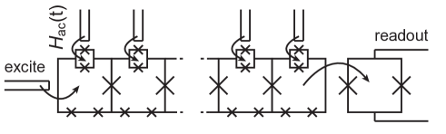
Figure 1: Schematic depiction of a superconducting qubit chain with controllable injection and readout as well as individual addressing for local modulation. By means of population measurements on a selected qubit, the presence of quantum coherence is inferred from dynamical localization effects, as described in the main text.

In general the superconducting qubit Hamiltonian can be written as $H_{s}=(\epsilon/2)\,\sigma^{z}+(\Delta/2)\,\sigma^{x}$. Depending on the particular qubit realization the parameters $\epsilon$ and $\Delta$ refer to different variables defining ”charge”, ”phase” or ”flux” qubits. The latter, also called ”persistent current qubit”, consists of a superconducting loop interrupted by three Josephson junctions, two with capacitance $C_{1}$ and the third with $C_{2}$ [25, 26, 20]. The values of the three Josephson junctions coupling constants, $E_{J,1}$ corresponding to capacitance $C_{1}$ and $E_{J,2}$ to capacitance $C_{2}$ respectively, are chosen so that the Josephson part of the Hamiltonian alone defines a bistable system. At a value of external magnetic flux $\Phi\approx 0.5\Phi_{0}$ ($\Phi_{0}=h/2e$ is the superconducting flux quantum), the system carries either a clockwise or counterclockwise persistent current, each generating an equal but opposite magnetic flux and defining the two possible states of this qubit. With an appropriate choice of the parameters $E_{J,1,2}$ and $C_{1,2}$, the barrier in phase space separating the left and right current states can be made low enough so that tunneling between the two classical states can occur. For the flux qubits $\Delta$ represents the tunneling amplitude, while the energy bias $\epsilon=-I_{p}(\Phi-0.5\Phi_{0})$ is proportional to the detuning $\Phi-0.5\Phi_{0}$, with $I_{p}$ the circulating current. The energies of the ground and first excited states are thus: $E_{\mp}=\mp\sqrt{\epsilon^{2}+\Delta^{2}}$.

For flux qubits, the most natural implementation for the interaction is through the mutual inductances between the loops. The flux generated by one qubit loop, which depends on its internal state, adds to the total flux picked up by the neighbouring qubits, thereby changing the energy biases of those qubits. The mutual inductance, and therefore the strength of the interaction ($J$), depends on the geometry of the qubit loops, specifically their size and their proximity to each other. The strength of the coupling can be enhanced in two steps. First by physically connecting the loops so that their persistent currents share a common line. In this case the kinetic inductance of the shared line adds to the geometrical inductance, where the former term can easily be the dominating part in the total interaction strength. To reach very strong coupling, for example to reach the regime $J>\Delta$, a fourth junction can be placed in the shared line. If the capacitance and Josephson junction coupling constant of this fourth junction are large compared to parameters of the qubit junctions, the single-qubit properties are not significantly altered, while still the interaction strength can be enhanced dramatically. Coupling strengths of several GHz are easily achieved. For the sake of the suggested experiments in this paper it is however not necessary to reach such high coupling values since the hopping inhibition between the qubits is enhanced in the regime where the hopping constant is smaller than the driving frequency, i.e. $J\ll\omega$ (see eqs. (15, 16) and explanations below those expressions).

In the experiment described in reference [27], it is demonstrated how the standard flux qubit design, for which only $\epsilon$ is a tunable parameter, can be extended to also have a tunable $\Delta$. The main change is that the smallest junction of the qubit is replaced by a small loop containing one junction in each arm, i.e. in a SQUID (Superconducting Quantum Interference device) geometry. The SQUID acts as a single junctions with tunable $E_{J}$, tuned by the flux penetrating the small loop. Local control lines can be used to change the flux through this loop, thereby controlling the $E_{J,2}$ of the qubit, and thus the $\Delta$. Fig. 1 shows a schematic of a possible implementation of a chain of strongly interacting flux qubits with tunable tunneling splitting $\Delta$. When the array of interacting superconducting flux qubits is operated at their corresponding degeneracy point the chain is described by a Hamiltonian of the form eq.(1), with $\omega_{i}=\Delta_{i}$. Typical values for the tunneling amplitudes are in the range of 5-20 GHz while nearest neighbour couplings $J\sim 200$ MHz. The residual next-to-nearest coupling is smaller than 10 MHz.

As far as the coupling to the environment is concerned, typically, noise sources that are located relatively far away from the chain couple to multiple or all qubits in the chain, for example magnetic coils, or some parts of the control and readout circuits. Noise sources that are located much closer, such as local control lines for the individual qubits, or microscopic noise sources in the materials surrounding the qubits, couple only, or mostly, to a single qubit. In this work we focus on the latter type: we suppose the array to be in contact with an external environment that acts locally on each qubit and can lead in principle to both pure dephasing and dissipation. In our model each qubit is coupled to its local environment via a spin-boson Hamiltonian of the form

$$H_{SB}=H_{s}+H_{b}+H_{s-b},$$ (19)

where the bath is modelled as a collection of harmonic oscillators, $H_{b}=\sum_{k}\omega_{k}\hat{a}_{k}^{\dagger}\hat{a}_{k}$ and system and bath couple linearly through the Hamiltonian [28]

$$H_{s-b}=\sigma_{z}^{i}\hat{X}_{i}.$$ (20)

Here $\hat{X}_{i}=\sum_{k}g_{k}(\hat{a}_{k}+\hat{a}_{k}^{\dagger})$ denotes the bath’s force operator. In the qubit eigenbasis and using the same symbols to denote the Pauli matrices in this new frame in order not to complicate notation, we can derive, using the standard assumptions, a Markovian master equation $\dot{\rho}=-i[H,\rho]+L_{\rm deph}(\varrho)+L_{\rm diss}(\varrho)$ for the qubit array where the coupling to the local environment is described in terms of Lindblad terms of the form [29, 30, 31]

$$L_{\rm deph}(\varrho)=\gamma_{\rm deph}\sum_{i=1}^{N}(2\sigma_{i}^{+}\sigma_{i}^{-}\varrho\sigma_{i}^{+}\sigma_{i}^{-}-\{\sigma_{i}^{+}\sigma_{i}^{-},\varrho\})$$ (21)

$$L_{\rm diss}(\varrho)=\gamma_{\rm diss}\sum_{i=1}^{N}(2\sigma_{i}^{-}\varrho\sigma_{i}^{+}-\{\sigma_{i}^{+}\sigma_{i}^{-},\varrho\}),$$ (22)

with $\gamma_{\rm deph}$ and $\gamma_{\rm diss}$ denoting the dephasing and dissipation rate, respectively, $\sigma_{i}^{\pm}=(\sigma_{i}^{x}\pm i\sigma_{i}^{y})/2$ acting on the $i$-th qubit of the chain and $\{\,,\,\}$ the anticommutation operation. The value of the noise rates in these expressions depends strongly on the selected qubit operating point via the parameter $\theta={\rm arctan}(\Delta/\epsilon)$. Measured values for $T_{1}=\gamma_{\rm diss}^{-1}$ range from 150 to 500 ns while pure dephasing times $(T_{2}^{\star})$ are typically around 300 ns. In the specific case where each qubit in the chain is operated at the degeneracy point, so that $\epsilon=0$ for every qubit, the pure dephasing term, which has a rate $\gamma_{\rm deph}\sim\cos(\theta)$ [29], cancels out and the chain is subject to dissipative noise only. This is the first parameter regime that we are going to analyze in the next section with the aim of unveiling coherent dynamics through dynamical localization effects in a driven chain. Later, still operating each qubit at its degeneracy point, we will relax the constraint of having only dissipation noise and we will consider possible dephasing effects arising from terms with the form of eq. (21).

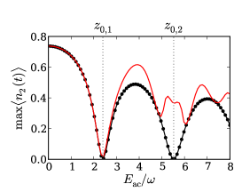
Figure 2: Coherent destruction of tunneling. Simulations corresponding to a $N=2$ chain with $\omega_{1}=\omega_{2}=10\rm GHz$ and hopping $J=10\rm MHz$. The black dots have been computed with $\omega=0.3\rm GHz$ and $H(t)=H_{z}(t)+H_{1}$ (see definitions in the text). The black line has been computed with $\omega=0.3\rm GHz$ and $H(t)=H_{z}(t)+H_{1}+H_{2}$. The red line has been computed with $\omega=2.0\rm GHz$ and $H(t)=H_{z}(t)+H_{1}+H_{2}$. The dissipation rate is the same in all curves $\gamma_{\rm diss}=1\rm MHz$. The dashed vertical lines represent the first $z_{0,1}\simeq 2.4048$ and second $z_{0,2}\simeq 5.5201$ zeros of the Bessel function $J_{0}(z)$.

IV Numerical Results

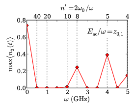
Figure 3: Resonance conditions. Simulations for a $N=2$ chain with $\omega_{1}=\omega_{2}=10\rm GHz$, $J=10\rm MHz$ and a dissipation rate $\gamma_{\rm diss}=1\rm MHz$. For each value of $\omega$, the electric field is fixed so that $E_{\rm ac}/\omega=z_{0,1}$, where $z_{0,1}\simeq 2.4048$ is the first zero of the Bessel function $J_{0}(z)$. The axis on the top represents some integer values $n^{\prime}=2\omega_{0}/\omega$ for which the resonance condition in the coupling constant $g^{\prime}$ is fulfilled.

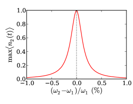
Figure 4: Effect of frequency inhomogeneities. Maximum value of the population transferred from qubit 1 to qubit 2 in a $N=2$ chain after a fixed time $t_{\max}=500\rm ns$. The frequency of the external field is $\omega=1.3\rm GHz$ and its magnitude is fixed so that $E_{\rm ac}/\omega=1.2$, far from the closest zero of the $J_{0}(z)$ Bessel function. The parameters of the qubits are $\omega_{0}=10\rm GHz$ and $J=10\rm MHz$. The dephasing and dissipation rates have been set to zero for clarity.

The phenomenon described above concerning the renormalization of the coupling constants in the interaction Hamiltonian eq.(4) under the effect of an external sinusoidal driving field can be clearly observed in fig. 2. There we study the dynamics of a chain consisting in two inductively coupled superconducting qubits operated at their degeneracy points, so that the (undriven) system Hamiltonian is given by eq.(1). In this case, as discussed before, the noise is purely dissipative when expressed in the rotated basis. The system is initialized so that only the first site is excited. The different curves correspond to the maximum value of the population that has been transferred from the first to the second qubit within a sufficiently long time interval ($1\,\mu{\rm s}$). The black line corresponds to an off-resonance situation ($\omega_{0}=10\,{\rm GHz}$, $\omega=0.3{\rm GHz}$, with no integer value $n^{\prime}$ such that $2\omega_{0}+n^{\prime}\omega=0$). In this situation the coupling of the contribution given by $H_{2}$ effectively renormalizes to zero and the dynamics is governed by the tight-binding term $H_{1}$. According to expression eq.(15), it is the Bessel function $J_{0}(E_{\rm ac}/\omega)$ which governs this behavior and when its argument $E_{\rm ac}/\omega$ coincides with one of its zeros, then the hopping between both qubits is suppressed. On the other hand, the red curve has been computed on a resonance situation ($\omega_{0}=10\,{\rm GHz}$, $\omega=2.0{\rm GHz}$, such that $2\omega_{0}+n^{\prime}\omega=0$ for $n^{\prime}=-10$). In this situation both couplings $g$ and $g^{\prime}$ in eqs.(15, 16) are in general different from zero and the total dynamics is hence more convoluted. Notice that the fact that both the red and black curves are indistinguishable to the eye for low values of $E_{\rm ac}/\omega$ is due to the slow buildup of the Bessel function $J_{n^{\prime}}(z)$ (with $n^{\prime}=10$) that governs the $H_{2}$ term. Finally, the black circles in fig. 2 have been computed using the same parameters that we used for the off-resonance situation but this time we explicitly excluded the contribution given by the $H_{2}$ terms. The fact that the black line and the black circles superimpose each other is a clear indication that the term $H_{2}$ effectively renormalizes to zero when the field is out of resonance with this term.

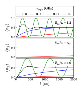
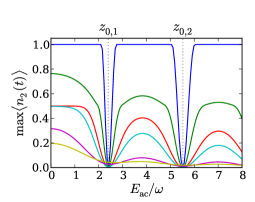
Figure 5: Effect of pure dephasing noise.(top) Population transfer from qubit 1 to qubit 2 in a $N=2$ chain and the following parameters: $\omega_{1}=\omega_{2}=10\rm GHz$, $J=10\rm MHz$, $\omega=1.3\rm GHz$. The dissipation rate has been set to zero ($\gamma_{\rm diss}=0.0$) for clarity and a new dephasing rate $\gamma_{deph}$ has been included ($\mathcal{L}_{\rm deph}\equiv\gamma_{\rm deph}\sum\mathcal{L}_{k}(\sigma^{z})$, with $\mathcal{L}_{k}(\sigma_{z})=\sigma_{k}^{z}\rho\sigma_{k}^{z}-\rho$). Each panel corresponds to a fixed value $z=E_{ac}/\omega$ with $z_{0,1}\simeq 2.4048$ the first zero of the Bessel function $J_{0}(z)$. (bottom) Maximum value of the population transferred to the second qubit in the time interval and with the same parameters as the figure on top and the following dephasing rates (in ${\rm GHz}$): $\gamma_{\rm deph}=0.0$ (blue),$\gamma_{\rm deph}=0.001$ (green),$\gamma_{\rm deph}=0.005$ (red),$\gamma_{\rm deph}=0.01$ (turquoise),$\gamma_{\rm deph}=0.05$ (cyan),$\gamma_{\rm deph}=0.1$ (yellow)

The existence of resonance conditions for the terms contributed by $H_{2}$ in expression eq.(4) is clearly illustrated in fig. 3, which has been evaluated with the same parameters as in fig. 2. We have however fixed the ratio $E_{\rm ac}/\omega=z_{0,1}$ with $z_{0,1}\simeq 2.4048$ the first zero of the Bessel function of order zero. With this constraint the population transfer induced by the terms contributed by $H_{1}$ in eq.(4) is completely suppressed. We have however the freedom to use different values of the driving field $\omega$ such that the term $H_{2}$ is either on- or off-resonance with the frequency $\omega_{0}$. We can clearly see in fig. 3 those values (compatible with the discrete grid used to sample the frequency $\omega$) where the resonance condition is fulfilled and a peak in the population transfer appears induced entirely by the terms in $H_{2}$.

As a result, the presence of a correction to the canonical Hamiltonian $H_{1}$ does not hinder the manifestation of localization effects. By appropriate tuning of the external driving we can select resonance conditions that lead to inhibition of transport and provide a fingerprint of the underlying coherent evolution. In fig. 4 we illustrate the effect of an inhomogeneous distribution of the tunneling amplitudes of the qubits within the chain. Not surprisingly, the presence of this sort of disorder in the array leads to a quick loss of contrast. However, the fact that the tunneling amplitude of superconducting flux qubits is actually tunable can provide mechanism to overcome this difficulty by minimizing or even suppressing the local disorder in the chain [33]. On the other hand, real implementations of interacting superconducting flux qubits typically result in interaction strengths differences of the order of few percents between different nearest neighbors. It is important to stress at this point that this differences have little effect in our previous discussion since they do not affect the resonance conditions in eqs.(15, 16), that are the key to the hopping inhibition effect presented in this work.

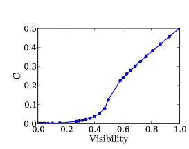
Figure 6: Quantum coherence in a N=2 chain. In this graph we plot the magnitude $C\equiv\max\sum_{i,j\neq i}{\rm abs}\big{(}\rho_{i,j}(t)\big{)}$ as a function of the visibility of the transport pattern (population fringes in Fig. 5). We have considered 27 values of the pure dephasing rate in a logarithmic scale from $\gamma_{\rm deph}=0.1{\rm GHz}$ $(C_{\rm max}\simeq 0)$ to $\gamma_{\rm deph}=0.0{\rm GHz}$ $(C_{\rm max}=0.5)$. For convenience we have fixed $\gamma_{\rm diss}=0$.

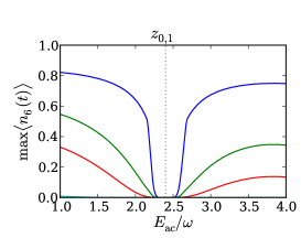
Figure 7: Hopping inhibition in a N=6 chain. Maximum value of the population transferred from the first qubit to the last one in a $N=6$ chain within a time interval of $2.8$ $\mu\rm s$. The frequency of the external field is $\omega=1.3\rm GHz$ and its magnitude is fixed so that $E_{\rm ac}/\omega=1.2$, far from the closest zero of the $J_{0}(z)$ Bessel function. The parameters of the qubits are $\omega_{1}=10\rm GHz$ and $J=10\rm MHz$.For this computation we have considered dissipation noise only, with the following rates (in ${\rm GHz}$): $\gamma_{\rm diss}=0.0001$ (blue), $\gamma_{\rm diss}=0.0005$ (green), $\gamma_{\rm diss}=0.001$ (red), $\gamma_{\rm diss}=0.005$ (turquoise, slightly visible).

In real implementations of superconducting flux qubits we should also expect deviations from a purely dissipative model of noise. This motivates the study of the effect of pure dephasing processes in our system. To this end we will introduce in the master equation a Lindblad term of the form given in eq.(22), with dephasing rate $\gamma_{\rm deph}$. To single out the effect of pure dephasing, we will take a vanishingly small dissipation rate, that is $\gamma_{\rm diss}=0$.
In fig. 5 we have studied how the transference of population in a chain is affected by pure dephasing noise terms. In fig. 5(up) we plot the dynamics of the population for different values of the dephasing rate, $\gamma_{\rm deph}=\{0.0,0.001,0.01,0.1\}{\rm GHz}$. It is worth remarking that the inclusion of these terms in the master equation leads to an asymptotic stationary state that is maximally mixed [34]. However, the transient dynamics still provides valuable information. It is remarkable to notice that even though the dephasing rapidly destroys the coherent oscillations of the population, still the renormalization of the hopping rate survives for surprisingly large values of $\gamma_{\rm deph}$. This fact can be clearly appreciated in the panel with $E_{\rm ac}/\omega=z_{0,1}$ where the hopping is strongly inhibited and still noticeable for dephasing rates as high as $\gamma_{\rm deph}=100$ ${\rm MHz}$. In fig. 5(down) we have plotted the same information in a more compact format. In this graph the effect of dephasing can be clearly seen to reduce the visibility of the population transfer oscillations (as a function of $E_{\rm ac}/\omega$ ). Nonetheless, as stated above, the hopping modulation is quite visible also in this graph even for large values of the dephasing rate.

The qualitative relation between the properties of the transport dynamics and the coherence in the system is illustrated in fig. 6. In this figure we have represented the coherence of the chain, quantified by the sum of the off diagonal elements of the density matrix $C\equiv\max\sum_{i,j\neq i}{\rm abs}\big{(}\rho_{i,j}(t)\big{)}$, as a function of the visibility of the population fringes depicted in fig. 5. For the sake of clarity we have used a purely dephasing noise since it uniquely affects the coherence terms of the density matrix. The main conclusions are however unaffected by including dissipation terms. We can see in this graph that the degree of quantum coherence of the system can be properly quantified by the transport schemes proposed in this work. For small values of the dephasing rate, the relation between coherence and visibility is indeed essentially linear. As a result, population measurements alone would allow, in the presence of a tunable driving, to detect signatures of quantum coherence in the system. The scalability of the procedure is illustrated in fig. 7 for an array of $N=6$ qubits, a system size that is currently untractable with tomographic schemes. As opposed to the previous graphs computed for $N=2$, now the one-excitation sector contains more than two eigenstates and hence the population dynamics is affected by more than one characteristic frequency. This results in a more convoluted dynamics and different possible protocols to measure the hopping inhibition. For this graph we have chosen to start with a chain where only the first qubit is initially on its excited configuration, we measure then the maximum population transferred to the last qubit within a time interval of $2.8\mu\textrm{s}$, long enough to allow the initial excitation to reach the end of the chain. Notice in this graph that the perfect hopping inhibition is again only achieved at the zeros of the corresponding Bessel functions. The fact that the hopping seems to vanish in an extended interval around this point is only a consequence of the interplay between the finite time interval used to perform the population measure and the arrival time required for a wavepacket created at the begining of the chain to reach its end (see ref.[15] for a thorough study of this topic), which increases as the hopping rate decreases.

V Conclusions

To summarize, we have analyzed the persistence of localization effects beyond exact tight binding Hamiltonians and beyond a closed system description. Introducing an a.c. interaction term of the form of eq.(2), we have seen that the original ZZ coupling, which provides the natural model for the actual coupling in superconducting architectures, can be effectively mapped into the Hamiltonian eq.(14) where the excitation-preserving and non-preserving terms are affected by two different renormalized couplings $g$ and $g^{\prime}$. We have seen that these effective couplings are determined by certain resonance conditions (for the coupling $g$ there is always a resonance for $n^{\prime}=0$, for $g^{\prime}$ the stronger condition $2\omega_{0}+n^{\prime}\omega=0$ is required) and, given that the resonance conditions are fulfilled, by the arguments of the Bessel functions that define these couplings. In conclusion, we have proposed a method that allows to tune independently two kinds of interaction of very different nature but with the common feature of leading to localization phenomena. These are shown to be useful for witnessing the coherent behaviour of coupled qubit arrays. As a proof of principle, using typical parameter regimes in chains of superconducting flux qubits, we have shown that transport inhibition can be qualitatively linked to the degree of coherence in the system. This type of experiments, which involve population measurements only, can provide a benchmark for quantum behaviour in systems whose complexity makes them unsuited for detailed tomographic analysis, ranging from arrays of self-assembled quantum dots [35] to coupled nanomagnets [36].

VI Acknowledgements

Financial support from the EU Integrated Project Q-Essence, STREP actions CORNER and PICC and the Humboldt Foundation is gratefully acknowledged. We thank H. Mooij, A. Rivas and B. Röthlisberger for helpful discussions and their comments on the precursor of this manuscript and to A. Bermúdez and M. Paternostro for their feedback on the current manuscript.

References

- [1] Dunlap D H and Kenkre V M 1986 Dynamic localization of a charged particle moving under the influence of an electric field Phys. Rev. B 34 3625
- [2] Holthaus M and Hone D W 1996 localization effects in ac-driven tight-binding lattices Phil. Mag. B 74 104-137
- [3] Audenaert K, Eisert J, Plenio M B and Werner R F 2002 Entanglement properties of the harmonic chain Phys. Rev. A 66 042327
- [4] Plenio M B, Hartley J and Eisert J 2004 Dynamics and manipulation of entanglement in coupled harmonic systems with many degrees of freedom New J. Phys. 6 36
- [5] Bose S 2007 Quantum communication through spin chain dynamics: an introductory overview Contemporary Physics 48 13
- [6] For a recent review, see S. Kohler, J. Lehmann and P. Häggi 2005 Phys. Rep. 406, 379
- [7] F. Grossmann, T. Dittrich, P. Jung, and P. Hänggi 1991 Coherent destruction of tunneling Phys. Rev. Lett. 67, 516
- [8] M. Grifoni and P. Hänggi, driven quantum tunneling, Phys. Rep. 304, 229 (1998).
- [9] Y. Kayanuma and K. Saito 2008 Coherent destruction of tunneling, dynamical localization and the Landau-Zehner formula Phys. Rev. A 77 010101(R)
- [10] Blümel R, Buchleitner A, Graham R, Sirko L, Smilansky U and Walther H 1991 Dynamical localization in the microwave interaction of Rydberg atoms: the influence of noise Phys. Rev. A 44 4521
- [11] Keay B J, Zeuner S, Allen S J Jr., Maranowski K D, Gossard A C, Bhattacharya U and Rodwell M J W 1995 Dynamic localization, absolute negative conductance, and stimulated, multiphoton emission in sequential resonant tunneling semiconductor superlattices Phys. Rev. Lett. 75 4102
- [12] Moore F L, Robinson J C, Bharucha C F, Williams P E and Raizen M G 1994 Observation of dynamical localization in atomic momentum transfer: a new testing ground for quamtum chaos Phys. Rev. Lett. 73 2974
- [13] Bharucha C F, Robinson J C, Moore F L, Sundaram B, Niu Q and Raizen M G 1999 Dynamical localization of ultracold sodium atoms Phys. Rev. E 60 3881
- [14] Creffield C. E. 2007, Quantum Control and Entanglement using Periodic Driving Fields, Phys. Rev. Lett. 99, 110501.
- [15] Galve F., Zueco D., Kohler S., Lutz E. and Hänggi P. 2009, Entanglement resonance in driven spin chains, Phys. Rev. A 79, 032332.
- [16] Kierig E et al 2008 Single-Particle Tunneling in Strongly Driven Double-Well Potentials Phys. Rev. Lett 100, 190405
- [17] Eckardt A and Holthaus M 2008 Avoided-Level-Crossing Spectroscopy with Dressed Matter Waves Phys. Rev. Lett 101, 245302
- [18] Fleming G R, Huelga S F and Plenio M B 2011 Focus on quantum effects and noise in biomolecules New. J. Phys 13 115002
- [19] Vaziri A and Plenio M B 2010 Quantum coherence in ion channels: resonances, transport and verification New J. Phys. 12 085001
- [20] Devoret M H, Wallraff A and Martinis J M 2004 Superconducting qubits: a short review arXiv:cond-mat/0411174, J. Q. You and F. Nori 2011 Atomic physics and quantum optics using superconducting circuits Nature 474, 589
- [21] Johnson M W et al 2011 Quantum annealing with manufactured spins Nature 473 194
- [22] M. Neeley et al 2010 Generation of Three-Qubit Entangled States using Superconducting Phase Qubits, Nature 467, 570
- [23] DiCarlo L et al 2010 Preparation and measurement of three-qubit entanglement in a superconducting circuit, Nature 467 574
- [24] Lucero E et al 2012 Computing prime factors with a Josephson phase qubit quantum processor, Nat. Phys. Advanced online publication, DOI: 10.1038/NPHYS2385
- [25] Mooij J E, Orlando T P, Tian L, van der Wal C H, Levitov L S, Lloyd S and Mazo J J 1999 A superconducting persistent current qubit Science 285 1036
- [26] Orlando T P, Mooij J E, Tian L, van der Wal C H, Levitov L S, Lloyd S, and Mazo J J 1999 Superconducting persistent-current qubit Phys. Rev. B 60 15398-15413
- [27] Paauw F G, Fedorov A, Harmans C J P M and Mooij J E 2009 Tuning the gap of a superconducting flux qubit Phys. Rev. Lett. 102 090501
- [28] Shnirman A, Makhlin Y and Schön G 2002 Noise and decoherence in quantum two-level systems Phys. Scr. T102 147
- [29] Tsomokos D I, Hartmann M J, Huelga S F and Plenio M B 2007 Entanglement dynamics in chains of qubits with noise and disorder New Journal of Physics 9 79
- [30] Rivas A, Plato A D K, Huelga S F and M.B. Plenio M B 2010 Markovian Master Equations: A Critical Study. New J. Phys. 12, 113032
- [31] Rivas A and Huelga S F, Open Quantum Systems. An Introduction. Springer Verlag, Heidelberg, 2011
- [32] Oxtoby N P, Rivas A, Huelga S F and Fazio R 2009 Probing a composite spin-boson environment New J. Phys. 11 063028
- [33] Recent work on tunable schemes is for instance reported in Bialczak R C et al 2011 Fast Tunable Coupler for Superconducting Qubits Phys. Rev. Lett. 106 060501
- [34] Rivas A, Oxtoby N P and Huelga S F 2009 Stochastic resonance phenomena in spin chains Eur. Phys. J. B 69, 51
- [35] Miller B T et al 1997 Few-electron ground states of charge-tunable self-assembled quantum dots Phys. Rev. B 56, 6764
- [36] Timco G A et al 2009 Engineering the coupling between molecular spin qubits by coordination chemistry, Nat. Nanotechnology 4, 173