Networks of noisy oscillators with correlated degree and frequency dispersion

Abstract

We investigate how correlations between the diversity of the connectivity of networks and the dynamics at their nodes affect the macroscopic behavior. In particular, we study the synchronization transition of coupled stochastic phase oscillators that represent the node dynamics. Crucially in our work, the variability in the number of connections of the nodes is correlated with the width of the frequency distribution of the oscillators. By numerical simulations on Erdös-Rényi networks, where the frequencies of the oscillators are Gaussian distributed, we make the counterintuitive observation that an increase in the strength of the correlation is accompanied by an increase in the critical coupling strength for the onset of synchronization. We further observe that the critical coupling can solely depend on the average number of connections or even completely lose its dependence on the network connectivity. Only beyond this state, a weighted mean-field approximation breaks down. If noise is present, the correlations have to be stronger to yield similar observations.

1 Introduction

In the last decade network science has become a field of research with increasing importance. This is mainly due to the fact that in principle any kind of coupling structure can be mapped to a network of specific complexity. In this way, one aims for understanding fundamental properties that networks with given structure may have in common. Besides a large variety of locally connected networks, the two most prominent examples were coined by Watts and Strogatz WaStr98 , and Barabási and Albert BarAl99 , who showed that various networks can be divided into so-called small-world or scale-free networks, respectively. In small-world networks, all the nodes typically have the same range of neighbor connections plus a few random shortcuts are established. In contrast, scale-free networks are characterized by a significant amount of “hub” nodes with a very large number of connections. Network science further owes its popularity to the growing relevance of interdisciplinary topics and to the advances in computer technology and science KlEguToSan03 .

One important topic is the study of the interplay between network topology and dynamics on the nodes, as impressively reviewed in AlBar02 ; New03 ; BocLaMoChHw06 ; BaBartVesp08 ; ArDiazKuMoZh08 . We pose the question, how correlations between connectivity and dynamics on the microscopic level affect the macroscopic behavior of a network. Such a connection between the numbers of links in a network and the functional ability of the node dynamics is evident and possibly caused by various reasons, for example by limited energy supply, restricted space or chemical resources, etc. Indeed, various types of neurons differ in the typical number of connections and firing rates VarChPanHaChk11 .

In order to approach the problem, we investigate the synchronization transition of phase oscillators in complex networks. The phenomenon of synchronization suits a
benchmark by virtue of its importance as a paradigmatic emergence of collective behavior, as outlined for instance in PikRosKu03 ; BalJaPoSos10 .

Only recently, Gómez-Gardeñes et al. showed that a special type of such a correlation can lead to an onset of synchronization resembling a first-order phase synchronization GogaGoArMo11 . This is remarkable, because the synchronization transition was always found to be of second order, if one only considers how different network topologies affect the dynamics. They instead identified the natural frequency of each node with its individual degree $\omega=k$, i.e., its number of connections. Furthermore, they interpolated between Erdös-Rényi random networks and scale-free networks. In this way it was found that the first-order nature of the synchronization transition appears only in scale-free networks; those networks are characterized by an unlimited dispersion of degrees. Hence, it was shown that a positive correlation between the dynamics of the oscillators and the large heterogeneity of the network has a drastic effect on the onset of synchronization.

In this paper, we consider a more general correlation between the degree and the frequency distributions; we relate the diversity of the frequencies to the degrees. Two different settings are generated, namely either positive or negative correlations between the degree of a node and how broad its oscillatory frequency varies from the mean one. We explore whether this kind of correlation with fixed average natural frequency is enough to yield a notable impact on the synchronization transition. In particular, we focus on the Erdös-Rényi random network model, which often serves as an important benchmark VarChPanHaChk11 . We show by simulations that the correlations can either support or impede the synchronizability. The results are supported by help of a weighted mean field theory SonnSchi12 which allows to formulate quantitative dependencies for the critical coupling within the validity of the approximative theory. We conclude by a qualitative discussion of our findings.

2 How degree-frequency correlations affect the synchronization transition

The most prominent model in studying synchronization phenomena is the Kuramoto model Kur84

$$\dot{\phi}_{i}(t)=\omega_{i}+\frac{\kappa}{N^{q}}\sum_{j=1}^{N}A_{ij}\sin\left(\phi_{j}(t)-\phi_{i}(t)\right)+\xi_{i}(t),$$ (1)

where $i=1,\ldots,N$, with natural frequency $\omega_{i}$ and phase $\phi_{i}(t)$ of oscillator $i$ at time $t$, respectively. The coupling strength is denoted by $\kappa$, the number of oscillators by $N$ and $q$ is a denseness parameter scaling the number of links with changing $N$;

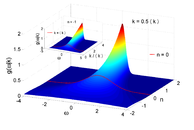
Figure 1: (Color online) Conditional Gaussian frequency distribution with $\sigma_{0}=1$ shown as a function of the correlation power $n$ and the relative degree $k/\langle k\rangle$ (inset).

for $q=0$ the network is sparse, while it is dense for $q=1$. Such a normalization is appropriate as long as all the degrees share the same scaling with the system size. Otherwise one may choose the maximum degree occurring in the network to guarantee an intensive coupling term ArDiazKuMoZh08 . We consider undirected and unweighted networks, in which case the adjacency matrix is symmetric with elements $A_{ij}=1$, if the units $i$ and $j$ are coupled, otherwise $A_{ij}=0$. Complex topologies of real-world networks can be encoded into the adjacency matrix, and decoded by counting all the degrees, which are given by

$$k_{i}=\sum_{j=1}^{N}A_{ij},$$ (2)

$k_{i}>0$ by definition. Calculating the probabilities of occurring degrees, yields the degree distribution $P(k)$. Various stochastic processes are brought together in the noise terms $\xi_{i}(t)$, such as the variability in the release of neurotransmitters or the quasi-random synaptic inputs from other neurons LiGarNeiSchi04 . The sum of stochastic influences is modeled by Gaussian white noise:

$$\langle\xi_{i}(t)\rangle =0,$$ (3)

$$\langle\xi_{i}(t)\xi_{j}(t^{\prime})\rangle =2D\delta_{ij}\delta(t-t^{\prime})\,.$$

The single parameter $D$ scales the noise intensity and is nonnegative. The angular brackets denote an average over different realizations of the noise.

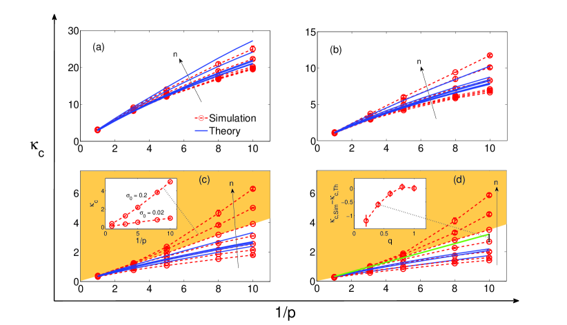
Figure 2: (Color online) The critical coupling strength depicted as a function of the inverse edge probability, which is proportional to the inverse average degree, see Eq. (7). Measurements are done via finite-size scaling analysis with systems of size $N=300,500,800,1200$ and $q=0.4$. Furthermore, a Gaussian frequency distribution is used with zero mean and standard deviation $\sigma_{n}(k_{i})$, where $\sigma_{0}=0.2$ (cf. Eq. (5)). Markers connected by dashed lines (red) show simulation results, while (blue) solid lines depict corresponding theoretical results, obtained by numerical integration. The thick solid (green) line in panel (d) is exactly obtained by Eq. (15) with $n=1,2$. The arrows show the direction of increasing $n$, from $n=-2$ to $n=4$. Panels (a)-(d) show results with decreasing noise intensity: (a) $D=1.5$, (b) $D=0.5$, (c) $D=0.05$, and (d) $D=0$. Inset in (c) presents $\kappa_{c}$ comparing $\sigma_{0}=0.2$ with $\sigma_{0}=0.02$ in case of $n=3$. Inset in (d) depicts the discrepancy $\kappa_{c,\mathrm{Sim}}-\kappa_{c,\mathrm{Th}}$ between simulation and theory as a function of the denseness parameter $q$ in case of $n=1$ and $p=0.1$. In the unshaded regions of (a)-(d) simulation results are accompanied by theoretical results, whereas in the shaded areas (orange) in (c) and (d) a superlinear growth of $\kappa_{c}$ cannot be described by our mean-field theory.

There are various possibilities how the individual oscillation frequencies and degrees can be correlated, including correlations between the mean values or the widths of the corresponding distributions. In Br08 ; FaHi09 the frequencies and degrees are assumed to be positively correlated, hence mean values and widths of the frequency and degree distributions are directly correlated. It is found that with increasing positive correlation, the oscillators are easier to synchronize. This phenomenon gives rise to the fact that one can observe an abrupt synchronization transition, if the natural frequencies and degrees are identified GogaGoArMo11 .

However, we remark that with respect to many real-world systems, one cannot observe a direct correlation between individual dynamics and connectivity. In neuronal networks for instance, a higher number of connections is not directly linked to a higher neuronal firing rate with respect to one cell type. This is due to the balance of inhibition and excitation VoSprZeClGer11 , where de- and acceleration compensate each other. Therefore, the central idea in this work is to consider correlations that are due to or affect only the variability in the degree or the frequency distribution, respectively. Hence, the mean values are not affected. To this end, we assume

$$\sqrt{\langle\omega_{i}^{2}\rangle-\langle\omega_{i}\rangle^{2}}=\sigma_{n}(k_{i}).$$ (4)

Each oscillator draws its natural frequency from the same distribution function, but with an individual standard deviation, given by the degree $k_{i}$. Here, $\sigma_{n}(k_{i})$ is an abbreviation for the power-law function

$$\sigma_{n}(k_{i})=\sigma_{0}\left(\frac{k_{i}}{\langle k\rangle}\right)^{n},n\in\mathbb{R}.$$ (5)

We call $n$ the correlation power; $\sigma_{0}$ stands for the original standard deviation without correlations. Eq. (5) gives rise to two different settings, namely either positive, $n>0$, or negative correlations, $n<0$. Note that for $k<\langle k\rangle$, i.e. nodes with degrees smaller than the average degree, the natural frequencies are the more sharply distributed around the mean frequency, the larger is $n$, while for $k>\langle k\rangle$ it is just the opposite case (see Fig. 1 for visualization).

We consider Erdös-Rényi like random networks that are constructed by assigning an edge probability

$$p_{e}=p\cdot N^{q-1},\ 0\leq p,q\leq 1$$ (6)

for any two of the $N$ nodes in the network with the scaling parameter $q$ introduced in Eq. (1). The further additional requirement is that besides the edge probability, each node is a priori connected to another randomly chosen one. In this way we guarantee that there are no isolated nodes, which are not interesting here, because they are not able to take part in the synchronization process and they only reduce the effective system size. Hence, the average degree reads

$$\langle k\rangle=2+pN^{q}\left(1-\frac{3}{N}\right),$$ (7)

which is approximately $pN^{q}$ for $q>0$ and $N\rightarrow\infty$. The first term in Eq. (7) stems from the random connections that are a priori chosen, whereas the second term is a result of the edge probabilities, Eq. (6). Higher moments and the degree distribution $P(k)$ are not known exactly. However, for large systems and $q>0$, the second term in Eq. (7) dominates and the degrees become binomially distributed New03 .

In our simulations, the stochastic differential equations are integrated up to $t=600$ with time step $\Delta t=0.05$ by using the Heun scheme. We consider a Gaussian frequency distribution with zero mean and standard deviation $\sigma_{n}(k_{i})$, where $\sigma_{0}=0.2$ (cf. Eq. (5)). Moreover, we discard the data up to $t=200$, by which transient effects are safely avoided. The statistical equilibria are further calculated as averages over at least $100$ different network realizations. The different network configurations do not differ only in the configuration of the connections, but the oscillators on the network differ as well: all the natural frequencies and the initial values of the phases change from one configuration to another.

In order to measure the critical coupling strength, we perform a finite-size scaling analysis SonnSchi12 ; HCK02 , where we take networks of size $N=300,500,800,1200$ with $q=0.4$. Fig. 2 displays the measured critical coupling strengths (red circles). As expected, both a larger noise intensity $D$ and a decrease of the number of connections, here parameterized by the inverse edge probability $1/p$, impedes the synchronizability. This causes the higher coupling strength $\kappa_{c}$ needed for the onset of synchronization (compare panels (a)-(d)).

Besides that, we observe that $\kappa_{c}$ increases with the correlation power $n$, which is by far not a foregone conclusion. One could have expected that both settings of correlation, i.e. $n<0$ and $n>0$ in (5), lead to a decrease of $\kappa_{c}$, because the latter marks the transition from the completely asynchronous to a partially synchronous state, and not to the completely synchronous state. For any correlation power, oscillators with a narrower frequency distribution appear which are easier to synchronize. Hence, a lower coupling strength would be needed for the onset of synchronization.

Instead, the uncorrelated case $n=0$ needs a critical coupling strength intermediate to the two settings with $n\neq 0$. Positive correlations require higher critical coupling strengths $\kappa_{c}$, negatively correlated networks can be easier synchronized, i.e. $\kappa_{c}$ decays.

First, we provide an intuitive explanation for this observation above; in the next section a mathematical reasoning will be given. The phenomenon of synchronization arises by virtue of interactions. Therefore, nodes with a larger degree $k>\langle k\rangle$ (hubs) are more crucial than nodes with a smaller degree $k<\langle k\rangle$ (compare with Ref. Per10 ). If the frequencies of these hubs are much broader spread around the average frequency, it is more difficult for the whole network to exhibit a synchronized oscillation. In other words, a population of oscillators is easier to synchronize, if the important nodes possess frequencies closer to the average frequency. In particular, for the case $n>0$, hubs are favored to have a great variability of frequencies, whereas sparsely linked nodes do the opposite. Necessary coupling for the onset of synchronization has to be larger than in the uncorrelated case. Differently for $n<0$, the less linked nodes own an increased variabilty compared to the uncorrelated case, but the hubs are now easier to synchronize since their frequencies are narrower distributed.

We further observe that the curves for different $n$ approach each other with increasing noise intensity $D$. This is due to the fact that a strong noise outweighs the diversity of the oscillators given by the frequency distribution; the effect of correlations is destroyed for large noise intensities and they become negligible.

Finally, it turns out to be beneficial to plot the critical coupling strength $\kappa_{c}$ as a function of the inverse edge probability $1/p$ as done in Fig. 2. In this way we observe two distinct regions: for small correlation power $n$, the critical coupling strength increases sublinearly as a function of $1/p$, while for large $n$, it increases superlinearly. In panel (d) a linear dependence is located between $n=1$ and $n=2$ for $D=0$. For larger noise intensities or smaller standard deviations $\sigma_{0}$ (compare inset in panel (c)), the separation between the two regions appears for larger correlation powers $n$. The shaded areas (orange) in panels (c) and (d) depict up to which $n$ we find the superlinear region by numerical simulations.

A linear dependence indicates that the onset of synchronization $\kappa_{c}$ solely depends on the mean degree $\langle k\rangle$, which is determined by $p$. Hence, for a certain $n_{c}$, the onset of synchronization seems to become independent of higher moments of the degree distribution. The heterogeneity in the network is masked by the correlations.

3 Theoretical considerations

In what follows, we discuss an approximation scheme SonnSchi12 that allows to reproduce analytically our observations above. We replace the random network by a fully connected network with random coupling weights that mimic the actual network structure. Requiring thereby the conservation of the individual degrees, $k_{i}=\sum_{j=1}^{N}\tilde{A}_{ij},\ i=1,\ldots,N$ (cf. Eq. (2)), the elements of the approximated adjacency matrix read

$$\tilde{A}_{ij}\,=\,k_{i}\,\frac{k_{j}}{\sum_{l=1}^{N}k_{l}}.$$ (8)

Inserting this into Eq. (1) yields a weighted mean-field approximation and effectively a one-oscillator description SonnSchi12 . In the following we consider the thermodynamic limit $N\rightarrow\infty$, where the system is conveniently described by the density $\rho(\phi,t|\omega,k)$, which is normalized according to $\int_{0}^{2\pi}\rho(\phi,t|\omega,k)\mathrm{d}\phi=1\ \forall\ \omega,k,t$.

For given degree $k$ and natural frequency $\omega$, $\rho(\phi,t|\omega,k)$ $\mathrm{d}\phi$ gives the fraction of oscillators having a phase between $\phi$ and $\phi+\mathrm{d}\phi$ at time $t$ (indices can be neglected, since all the nodes are assumed to be statistically identical). The completely asynchronous state is given by $\rho(\phi,t|\omega,k)=1/(2\pi)\ \forall\ \omega,k,t$ and we aim at calculating the critical coupling strength, where it loses its stability, which marks the onset of synchronization. The linear stability of the completely asynchronous state is characterized by a single real-valued eigenvalue $\lambda$ given by a self-consistent equation SonnSchi12 :

$$1=\frac{\kappa}{2N^{q}\langle k\rangle}\int_{-\infty}^{+\infty}\mathrm{d}\omega^{\prime}\sum_{k^{\prime}}\frac{(\lambda+D)k^{\prime 2}}{(\lambda+D)^{2}+\omega^{\prime 2}}P\left(\omega^{\prime},k^{\prime}\right)\ .$$ (9)

The sum over $k^{\prime}$ covers all possible degrees, which could be further approximated by an integral. The joint probability density $P(\omega,k)$ takes into account the possibility of correlations between the frequencies and degrees. In the derivation of Eq. (9) we assume that, with regard to the $\omega$-dependency, $P(\omega,k)$ has a single maximum at frequency $\omega=0$ (this choice is always possible due to the rotational symmetry) and is symmetric with respect to it.

The critical condition $\lambda=\lambda_{c}=0$ yields the critical coupling strength

$$\kappa_{c}=2N^{q}\langle k\rangle\left[\int_{-\infty}^{+\infty}\mathrm{d}\omega^{\prime}\sum_{k^{\prime}}\frac{Dk^{\prime 2}}{D^{2}+\omega^{\prime 2}}P\left(\omega^{\prime},k^{\prime}\right)\right]^{-1}\ .$$ (10)

This equation is not valid in the noise-free case, where one has to take the limit $\lambda\to 0^{+}$ in Eq. (9) with $D=0$ resulting in

$$\kappa_{c}=2N^{q}\langle k\rangle\left[\pi\sum_{k^{\prime}}k^{\prime 2}P\left(0,k^{\prime}\right)\right]^{-1}\ .$$ (11)

To see this, note that $\lim_{\lambda\to 0^{+}}\int_{-\infty}^{+\infty}\mathrm{d}\omega^{\prime}\lambda/\left(\lambda^{2}+\omega^{\prime 2}\right)=\pi\int_{-\infty}^{+\infty}\mathrm{d}\omega^{\prime}\delta(\omega^{\prime})$ StrMir91 .

Assuming a given degree distribution $P(k)$, the joint frequency and degree distribution separates as $P(\omega,k)\equiv g(\omega|k)P(k)$ with the conditional frequency distribution $g(\omega|k)$. It gives the probability that an oscillator at a node with degree $k$ has the natural frequency $\omega$. It includes the relation (4), i.e. the correlations between the degree and the frequency variation.

First, in accordance with the numerics above, we consider a Gaussian frequency distribution:

$$g_{\rm{gauss}}(\omega|k)=\frac{1}{\sqrt{2\pi}\sigma_{n}(k)}\mathrm{e}^{-\frac{1}{2}\frac{\omega^{2}}{\sigma_{n}(k)^{2}}}.$$ (12)

and $\sigma_{n}(k)$ is expressed by (4). Taking the integral, we derive the critical coupling strength (10):

$$\kappa_{c,\rm{gauss}}= \ 2\sqrt{\frac{2}{\pi}}\sigma_{0}N^{q}\langle k\rangle^{1-n}$$ (13)

$$\times\left\langle k^{2-n}\operatorname{erfc}\left(\frac{D}{\sqrt{2}\sigma_{n}(k)}\right)\exp\left(\frac{D^{2}}{2\sigma_{n}(k)^{2}}\right)\right\rangle^{-1},$$

which is an intensive parameter and scales with the variation of frequencies for small $\sigma_{0}$ (see inset in panel (c) of Fig. 2).

By calculating $\mathrm{d}\kappa_{c}/\mathrm{d}n$, we want to validate that the critical coupling strength indeed grows with the correlation power, as stated in the previous section. To this end, we use Eq. (13) and arrive at a sufficient condition for $\mathrm{d}\kappa_{c,\rm{gauss}}/\mathrm{d}n>0$, namely

$$\frac{2}{\sqrt{\pi}}y>\left(2y^{2}-1\right)\exp\left(y^{2}\right)\operatorname{erfc}\left(y\right),$$ (14)

with $y=D\left(\langle k\rangle/k\right)^{n}/\left(\sqrt{2}\sigma_{0}\right)$. Since we have $y>0$, the inequality (14) is true; in fact, the right-hand side divided by $y$, approaches $2/\sqrt{\pi}$ from below for $y$ going to infinity.

In the noise-free case $D=0$ we find

$$\kappa_{c,\rm{gauss}}(D=0)=2\sqrt{\frac{2}{\pi}}\sigma_{0}N^{q}\frac{\langle k\rangle^{1-n}}{\langle k^{2-n}\rangle}.$$ (15)

Interestingly, for $n=1$ and $n=2$, we get the same critical coupling strength growing inversely to the average degree:

$$\kappa_{c,\rm{gauss}}(D=0,n=1,2)=2\sqrt{\frac{2}{\pi}}\frac{\sigma_{0}}{p}$$ (16)

in the thermodynamic limit (cf. Eq. (7)). In Fig. 2 the solid blue lines describe the critical coupling strength as given by numerical integration of Eqs. (13) or (15) with a binomial degree distribution and system size $N=1000$. In panel (d) for $n=1,2$, instead of the numerical integration of Eq. (15), the exact expression (16) is shown (thick green line). The agreement between theory and simulation is satisfactory in (a)-(d) and confirms the previous observations. The weighted mean-field approximation does not yield superlinear dependencies. Simulation results in the shaded (orange) areas in panels (c) and (d) are therefore not covered by the theory; the validity of the approximation restricts to correlation strengths with sub- and linear growth of $\kappa_{c}$. For large noise intensities $D$ the theory overestimates the critical coupling strength $\kappa_{c}$, irrespective of the correlation power $n$, but this may turn into the opposite case when decreasing $D$ depending on $n$. In summary, there seems to be some particular noise values where the agreement between theory and simulation is particularly good. As presented in the inset of panel (d), deviations between the results from the numerical simulations $\kappa_{c,\mathrm{Sim}}$ and from the weighted mean-field theory $\kappa_{c,\mathrm{Th}}$ can be further reduced by increasing $q$. Hence, more densely connected networks are better reflected by the theory.

4 Generalizations

The network model under consideration constitutes already a generalized model, since it allows to interpolate between sparse and dense random networks. Here we discuss two further generalizations, namely other frequency distributions and different normalization variants of the coupling term, cf. Eq. (1). In particular, we consider now a Lorentzian and a uniform frequency distribution:

$$g_{\rm{lorentz}}(\omega|k) =\frac{\sigma_{n}(k)}{\pi}\frac{1}{\sigma_{n}(k)^{2}+\omega^{2}},$$ (17)

$$g_{\rm{uni}}(\omega|k) =\frac{1}{2\sqrt{3}\sigma_{n}(k)},\ |\omega|\leq\sqrt{3}\sigma_{n}(k),$$

Note that in case of the Lorentzian, $\sigma_{n}(k)$ does not have the meaning of a standard deviation, instead it is the scale parameter for the width of the distribution. We further introduce a generalized normalization $\mathcal{N}(k)$ instead of $N^{q}$, which can be a function of the degree $k$. Then we find for the critical coupling strength:

$$\kappa_{c,\rm{lorentz}}=2\langle k\rangle\left\langle\frac{k^{2}}{\mathcal{N}(k)}\frac{1}{D+\sigma_{n}(k)}\right\rangle^{-1},$$ (18)

$$\kappa_{c,\rm{uni}}=2\sqrt{3}\sigma_{0}\langle k\rangle^{1-n}\left\langle\frac{k^{2-n}}{\mathcal{N}(k)}\arctan\left(\frac{\sqrt{3}\sigma_{n}(k)}{D}\right)\right\rangle^{-1}.$$

Let us now specify the normalization $\mathcal{N}(k)$ by considering two cases: $\mathcal{N}(k)=\langle k\rangle$ and $\mathcal{N}(k)=k$. In the first case, one assumes again that the system-size scaling of the number of connections is the same for all nodes. In order to distinguish the two normalizations, we denote the critical coupling strength by $\kappa_{a}$ or $\kappa_{w}$, respectively. In the noise-free case $D=0$ we obtain, in contrast to (15), the following relations with the same constant of proportionality $C$:

$$\kappa_{a}=C\sigma_{0}\frac{\langle k\rangle^{2-n}}{\langle k^{2-n}\rangle},\ \kappa_{w}=C\sigma_{0}\frac{\langle k\rangle^{1-n}}{\langle k^{1-n}\rangle},$$ (19)

irrespective of whether we consider a Gaussian, a Lorentzian or a uniform frequency distribution. Only the constant of proportionality $C$ is different, namely $C_{\rm{gauss}}=2\sqrt{2/\pi}\approx 1.60$, $C_{\rm{lorentz}}=2$ or $C_{\rm{uni}}=4\sqrt{3}/\pi\approx 2.21$.

Again we find a disappearance of network effects for specific correlation powers. The phenomenon is even more pronounced here, since $\kappa_{a}$ becomes a constant for $n=1,2$. Moreover we see that $\kappa_{w}(n)=\kappa_{a}(n+1)$. Correspondingly, $\kappa_{w}$ becomes a constant for $n=0,1$. It has been pointed out in the literature, e.g. in ArDiazKuMoZh08 , that the additional weight introduced by the normalization $\mathcal{N}(k)=k$ can mask the heterogeneity of the network. Our results constitute a generalization of this statement. Preliminary numerical simulations can reproduce our theoretical result $\kappa_{w}(n)=\kappa_{a}(n+1)$, while the point where the onset of synchronization loses its dependence on the network connectivity is found to appear at smaller values of $n$ than predicted by the theory.

5 Conclusion

We assumed correlations between the degree number in a complex betwork and the variance of frequencies of phase oscillators belonging to the nodes. By estimating numerically and analytically the critical coupling strength that marks the onset of synchronization, we were able to show that correlations can favor as well as impede the ability of creating coherent network oscillations. In both scenarios, the behavior of hubs (nodes with large degree) plays a dominant role. Stronger coupling is necessary, if the hubs have broadly distributed frequencies. The onset of synchonization is shifted up, despite the fact that the less linked nodes possess a narrower frequency band and would, taken separately, synchronize at lower couplings. The opposite happens in case that hubs have narrowed distributions. We have further demonstrated that noise acting on the frequencies plays a crucial role; correlation effects become maximally strong in case of vanishing noise intensity.

We mention that our analysis was performed for edge probabilities $p$ larger than $0.1$. In this region we have found a good applicability of the weighted mean field theory proposed in SonnSchi12 . Analytical results agree satisfactorily with numeric ones for sufficiently large noise $D$ or not too strong correlation powers $n$ and dense enough scaling of the links $q>0$ in particular, as long as the critical coupling grows sub- or linearly with $1/p$. Beyond a certain denseness parameter for given correlation power, the weighted mean-field approximation breaks down.

In a recent preprint SkSuTaRes12 , the masking of the structural heterogeneity was independently found for another type of correlation.

- (1) D. J. Watts and S. H. Strogatz. Nature, 393:440–442, 1998.
- (2) A.-L. Barabási and R. Albert. Science, 286(5439):509, 1999.
- (3) K. Klemm, V. M. Eguiluz, R. Toral, and M. SanMiguel. Phys. Rev. E, 67(2):026120, 2003.
- (4) R. Albert and A.-L. Barabási. Rev. Mod. Phys., 74(1):47–97, 2002.
- (5) M. E. J. Newman. SIAM Rev., 45(2):167–256, 2003.
- (6) S. Boccaletti, V. Latora, Y. Moreno, M. Chavez, and D.-U. Hwang. Phys. Rep., 424:175–308, 2006.
- (7) A. Barrat, M. Barthélemy, and A. Vespignani. Dynamical Processes on Complex Networks. Cambridge Univ. Press, U. K., 2008.
- (8) A. Arenas, A. Díaz-Guilera, J. Kurths, Y. Moreno, and C. Zhou. Phys. Rep., 469:93–153, 2008.
- (9) L. R. Varshney, B. L. Chen, E. Paniagua, D. H. Hall, and D. B. Chklovskii. PLoS Comput. Biol., 7(2):e1001066, 2011.
- (10) A. Pikovsky, M. Rosenblum, and J. Kurths. Synchronization: A universal concept in nonlinear sciences. Cambridge Univ. Press, U. K., 2003.
- (11) A. Balanov, N. Janson, D. Postnov, and O. Sosnovtseva. Synchronization: From Simple to Complex. Springer-Verlag, Berlin, Heidelberg, New York, Tokyo, 2010.
- (12) J. Gómez-Gardenes, S. Gómez, A. Arenas, and Y. Moreno. Phys. Rev. Lett., 106:128701, 2011.
- (13) B. Sonnenschein and L. Schimansky-Geier. Phys. Rev. E, 85:051116, 2012.
- (14) Y. Kuramoto. Chemical Oscillations, Waves, and Turbulence. Springer-Verlag, Berlin, Heidelberg, New York, Tokyo, 1984.
- (15) B. Lindner, J. García-Ojalvo, A. Neiman, and L. Schimansky-Geier. Phys. Rep., 392:321–424, 2004.
- (16) M. Brede. Phys. Lett. A, 372:2618, 2008.
- (17) J. Fan and D. J. Hill. Enhancement of Synchronizability of the Kuramoto Model with Assortative Degree-Frequency Mixing. In J. Zhou, editor, Complex Sciences, volume 5, pages 1967–1972. Springer-Verlag, Berlin Heidelberg, 2009.
- (18) T. P. Vogels, H. Sprekeler, F. Zenke, C. Clopath, and W. Gerstner. Science, 334:1569, 2011.
- (19) H. Hong, M. Y. Choi, and B. J. Kim. Phys. Rev. E, 65:026139, 2002.
- (20) T. Pereira. Phys. Rev. E, 82:036201, 2010.
- (21) S. H. Strogatz and R. E. Mirollo. J. Stat. Phys., 63(3/4):613–635, 1991.
- (22) P. S. Skardal, J. Sun, D. Taylor, and J. G. Restrepo. arXiv:1208.4540 [nlin.AO], 2012.