Asymptotically Matched Spacetime Metric for Non-Precessing, Spinning Black Hole Binaries

Abstract

We construct a closed-form, fully analytical $4$-metric that approximately represents the spacetime evolution of non-precessing, spinning black hole binaries from infinite separations up to a few orbits prior to merger. We employ the technique of asymptotic matching to join a perturbed Kerr metric in the neighborhood of each spinning black hole to a near-zone, post-Newtonian metric farther out. The latter is already naturally matched to a far-zone, post-Minkowskian metric that accounts for full temporal retardation. The result is a $4$-metric that is approximately valid everywhere in space and in a small bundle of spatial hypersurfaces. We here restrict our attention to quasi-circular orbits, but the method is valid for any orbital motion or physical scenario, provided an overlapping region of validity or buffer zone exists. A simple extension of such a metric will allow for future studies of the accretion disk and jet dynamics around spinning back hole binaries.

1 Introduction

A closed-form, analytic understanding of the two-body problem in General Relativity has proven quite elusive. From the point of view of gravity, this holds true for Newtonian stars described by Newtonian gravity, but even more so for binary compact objects, such as black holes (BHs) and neutron stars (NSs), in the last stages of inspiral and merger. Perhaps, this can be traced to the fact that the “two-body problem” in General Relativity is really a “one-spacetime” problem, where the orbital dynamics cannot be easily separated from the spacetime dynamics. Fortunately, the breakthroughs in numerical relativity [1, 2, 3] have now made possible to fully compute the dynamics of any binary BH (BBH) spacetime for a wide variety of mass ratios and spins parameters. However, these calculations are still very expensive, and therefore are limited to few orbital evolutions with the BHs starting at relatively close separations.

A closed-form, analytic understanding of the full spacetime in the inspiral regime would be extremely useful to study a variety of astrophysical phenomena that require a large number of orbits. The study of the dynamics of accretion disks around BBHs and of any associated electromagnetic emission and jets is a good example. With this goal in mind, we develop an asymptotically matched spacetime metric for non-precessing, spinning BBHs. Further motivation for our work is described in [4].

Our work builds on important previous analytic perturbative techniques, which have been successfully developed to tackle the BBH problem. Post-Newtonian (PN) theory (see, e.g., [5] for a review) can be successfully used to describe the motion of the BBH in the early stages of the inspiral. Here, all fields are perturbatively expanded in a slow motion $v/c\ll 1$ and weak field $GM/(rc^{2})\ll 1$ approximation . Close to each of the BHs, one can use perturbation theory, where all fields are treated as small deformations of a known analytic solution, such as the Schwarzschild or Kerr metric.

During the late stages of a binary BH, however, the whole spacetime cannot be described using a single perturbative method. For clarity, let us classify different spatial regions on a spacelike hypersurface into zones [6] (see Figure 1 and Table 1 for a BBH). The inner zone (IZ) is defined as the region close enough to either BH that the metric can be treated as a perturbation of the Kerr spacetime due to some external universe [7, 8, 9, 10, 11, 12]. The near zone (NZ) is defined as the region both far enough from either BH that the metric can be perturbatively expanded in a weak-field approximation, while simultaneously much smaller than a gravitational wavelength, so that time retardation can be treated perturbatively [5]. The far zone (FZ) is defined as the region sufficiently far away from the center of mass of the system (much farther than a gravitational wavelength) that the metric can be modeled via a multipolar post-Minkowskian expansion [5]. In each of these zones, one can construct an approximate $4$-metric, in some coordinate system well-adapted to that particular zone, and in terms of certain physical parameters, like the BH masses and spins.

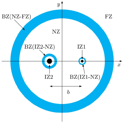
Figure 1: BH1 and BH2 are denoted by solid black dots, where the orbital separation is $b$. The BZs are denoted with cyan shells, the outer one representing the FZ/NZ BZ and the two inner ones representing the NZ/IZ BZs (see also Table 1). The circular nature of these buffers zones is because the diagram is schematic; in practice, one expects these to be distorted. The IZ, NZ and FZ are also shown in the figure.

Asymptotic matching is the mathematical technique that allows one to relate the coordinates and parameters used in adjacent zones inside of a common overlapping region of validity, or buffer zone (BZ) (see Figure 1 and Table 1). Formally, asymptotic matching requires that one set the asymptotic expansion of approximate $4$-metrics inside the BZ equal to each other. This yields a system of differential and algebraic equations for the coordinate and parameter transformation that relates adjacent approximate metrics. After applying such a transformation, one can then join the approximate metrics with carefully constructed transition functions to obtain an approximate global metric.

Such an approximate global metric is ideal as initial data, because in practice asymptotic matching is carried in the neighborhood of some fiducial time $t_{0}$, i.e., the BZ is the product of a $3$-torus with a small segment of the real (temporal) line. Alvi [13, 14] was the first to attempt such an initial data construction, but ended up carrying out asymptotic patching rather than matching . Yunes et al. [15, 17, 18, 19] succeeded in carrying out matching for non-spinning BBHs and this data has recently been evolved in [20] (see also [21] for numerical evolutions of superposed tidally perturbed BHs).

Table 1: $r_{\rm in}$ and $r_{\rm out}$ denote the approximate inner and outer boundary radius, respectively, while “Region” stands for the spatial domain in which the BZs exist. $r_{A}$ is the distance from a $A$th BH with mass $m_{A}$, $r$ is the distance from the center of mass, and $b$ and $\lambda$ are the orbital separation and the gravitational wavelength, respectively.

Zone	$r_{\rm in}$	$r_{\rm out}$	Region
IZ BH1 ($r_{1}$)	$0$	$\ll b$	$\cdot$
IZ BH2 ($r_{2}$)	$0$	$\ll b$	$\cdot$
NZ ($r_{A}$)	$\gg m_{A}$	$\ll\lambda$	$\cdot$
FZ ($r$)	$\gg b$	$\infty$	$\cdot$
IZ-NZ BZ	$\cdot$	$\cdot$	$m_{A}\ll r_{A}\ll b$
NZ-FZ BZ	$\cdot$	$\cdot$	$b\ll r\ll\lambda$

In this paper, we extend the calculation in [15, 17, 19] to non-precessing, spinning BBHs in a quasi-circular orbit, with BH spins aligned or anti-aligned with the orbital angular momentum. The NZ and FZ are modeled via the standard PN approximation [22, 23, 24, 25, 26] (and references therein). The IZ around each BH is modeled as a Kerr spacetime with a leading-order vacuum perturbation, following Yunes and González [27]. The IZ metrics are cast in a coordinate system that is both horizon-penetrating and harmonic [28]. This simplifies the matching and allows for excision of the singularities.

We first carry out asymptotic matching in the non-spinning limit. Our results for the matching coordinate and parameter transformation differ from those of [15, 17, 19] because our IZ metrics differ by a gauge transformation. We then carry out asymptotic matching for an aligned or counter-aligned, arbitrarily spinning binary. The matching coordinate and parameter transformation are not affected by spin to the matching order studied. Asymptotically matching the metrics to higher order would introduce spin-dependent terms in the coordinate and parameter transformation, but this would require perturbed Kerr metrics valid to higher multipolar order in the IZs. Once asymptotic matching has been carried out, we stitch the different metrics via appropriate transition functions, thus obtaining a global approximate metric.

We verified that this metric is indeed an approximate solution to the Einstein equations. One might be worried that the stitching procedure introduced errors in the global metric that are larger than those inherently contained in any of the approximate metrics. This is not the case because the transition functions used satisfy the Frankenstein theorems of [18]. We verified this qualitatively by visually inspecting different components and the volume element of the global metric. We then verified this quantitatively by evaluating the Ricci scalar for the global metric on a $t=0$ spatial hypersurface. We find that the global metric is an approximate solution to the Einstein equations for all values of spin considered, provided the binary orbital separation is sufficiently large, so that BZs in which to carry out asymptotic matching exist. We further verified that as this orbital separation is increased, the satisfaction of the Einstein equation increases at the expected rate (given by the matching order).

Such a global metric is technically valid close to a $t=0$ spatial hypersurface because the BZ in which matching is carried out is formally a small $4$-volume about this hypersurface. One can, however, extend this global metric to a dynamical global representation of the full spacetime, following the procedure in [29]. This scheme essentially consists of using a sequence of temporally-spaced global metrics and properly gluing these together. Such a spacetime was successfully employed to model how the inspiral of BBHs affects accretion disks [4].

The remainder of this paper is organized as follows. In section 2, we summarize how the metrics of each zone are constructed. In section 3, we first redo asymptotic matching between IZ and NZ metrics in the non-spinning case but using an IZ metric different from the one used in [15, 17, 18, 19], and then extend it to the spinning case. We present some technical details and supplementary analyses in the appendices. In A, we review how this paper is related to [27], and extend the formulation by including the $m=0$ azimuthal mode. In B, we present a detailed and complete analysis of asymptotic matching. In C, we discuss how to glue the metrics in each zone with transition functions. In D, we summarize some higher order metrics which are available for the non-spinning case in the supplemental material of [19].

All throughout, we use the following conventions, following mostly Misner, Thorne and Wheeler [30]. We use the Greek letters $(\alpha,\beta,\cdots)$ to denote spacetime indices, and Latin letters $(i,j,\cdots)$ to denote spatial indices. The metric is denoted $g_{\mu\nu}$ and it has signature $(-,+,+,+)$. We use geometric units, with $G=c=1$.

2 Approximate Metrics

2.1 Inner Zone

The metric in either IZ is approximated with a Kerr solution plus a linear vacuum perturbation [27]:

$$g_{\mu\nu}^{{\mbox{\tiny IZ}}}=g_{\mu\nu}^{{\mbox{\tiny Kerr}}}+h_{\mu\nu}^{{\mbox{\tiny IZ}}}\,;$$ (1)

the construction of $h_{\mu\nu}^{{\mbox{\tiny IZ}}}$ is difficult but essential for our purposes. Vacuum perturbations of Schwarzschild have been studied, for example, in [31], where one can use the Regge-Wheeler-Zerilli-Moncrief formalism [32, 33, 34]. When considering the Kerr background, however, the perturbation equations do not easily decouple, as tensor spherical harmonics are not eigenfunctions of the angular sector of the linearized Einstein equations [35]. Instead one has to carry out the so-called Chrzanowski procedure [36], amended by Wald [37] and by Kegeles and Cohen [38], as we describe below.

In the Chrzanowski procedure [36], the vacuum perturbation $h_{\mu\nu}^{{\mbox{\tiny IZ}}}$ is obtained from a so-called Hertz potential $\Psi$ via

$$h_{\mu\nu}^{{\mbox{\tiny IZ}}} =\hat{h}_{\mu\nu}\left[\Psi\right]\,,$$ (2)

where $\hat{h}_{\mu\nu}\left[\cdot\right]$ is a differential operator. This potential must satisfy a certain non-linear differential equation with a source given by the Newman-Penrose scalar $\psi_{0}$ (or $\psi_{4}$ depending on the radiation gauge used). This differential relation can be inverted through the Teukolsky-Starobinski relation to yield $\Psi$ in terms of $\psi_{0,4}$ ([37, 39, 40]). Thus, the construction of a metric perturbation reduces to finding an appropriate solution for the Newman-Penrose scalar.

The Newman-Penrose scalar must, of course, satisfy the Teukolsky equation, but when the source is a slowly-varying external universe (as is the case when the perturbation is due to a BH binary companion in a circular orbit with large semi-major axis), this equation can be solved perturbatively. One first performs a harmonic decomposition of $\psi_{0}$ in terms of spin-weight $2$ spherical harmonics (or $\psi_{4}$ in terms of spin-weight $-2$ spherical harmonics), ${}_{2}Y^{\ell m}$:

$$\psi_{0}=\sum_{\ell,m}R_{\ell m}(r)z_{\ell m}(v)\;{}_{2}Y^{\ell m}(\theta,\phi)\,,$$ (3)

where the radial and temporal dependence are product decomposed in terms of unknown real functions $R_{\ell m}(r)$ and unknown complex functions $z_{\ell m}(v)$, where $v$ is the advanced Kerr-Schild time coordinate. The latter can be written in terms of certain combinations of electric and magnetic tidal tensor components, which characterize the perturbations of the external universe. To leading order in a small-hole/slow-motion approximation [41] in BH perturbation theory, it suffices to keep only the $\ell=2$ quadrupolar deformation (see also A). The radial functions are then required to satisfy the (time-independent) Teukolsky equation, which one can solve in terms of hypergeometric functions [41, 27]. This means that $z_{\ell m}$ is constant or slowly varying in time. With the Newman-Penrose scalars under control, one then proceeds to compute the Hertz potential $\Psi$, and from that, the metric perturbation. Reference [27] provides explicit expressions for $g_{\mu\nu}^{{\mbox{\tiny IZ}}}$ in Boyer-Lindquist (BL) coordinates.

For ease during the matching procedure, one wishes to express the IZ metric in a coordinate system that closely parallels that used in the NZ. We thus transform the IZ metric from BL coordinates ($t_{\rm BL},\,r_{\rm BL},\,\theta_{\rm BL},\,\phi_{\rm BL}$) to harmonic, horizon-penetrating coordinates ($T,\,X,\,Y,\,Z$). Harmonic coordinates are those that satisfy $\square x^{\mu}=0$, which of course defines a class of coordinate systems. Several coordinate transformations between BL and different members of this class were developed in [42, 43, 28, 44, 45, 46, 47]; we here employ one such transformation that leads to harmonic coordinates that are also horizon-penetrating [28], namely

$$T=t_{\rm BL}+\frac{r_{+}^{2}+A^{2}}{r_{+}-r_{-}}\,\ln\left|\frac{r_{\rm BL}-r_{+}}{r_{\rm BL}-r_{-}}\right|\,,\;Z=(r_{\rm BL}-M)\cos\theta_{\rm BL}\,,$$

$$X+i\,Y=(r_{\rm BL}-M+i\,A)e^{i\,\phi_{\rm IK}}\,\sin\theta_{\rm BL}\,;\;\phi_{\rm IK}=\phi_{\rm BL}+\frac{A}{r_{+}-r_{-}}\,\ln\left|\frac{r_{\rm BL}-r_{+}}{r_{\rm BL}-r_{-}}\right|\,,$$ (4)

where $A=S/M$ is the dimensional Kerr spin parameter associated with the Kerr background with spin $S$, and $M$ is the mass of the Kerr background, with $r_{\pm}=M\pm\sqrt{M^{2}-A^{2}}$ the location of the unperturbed inner and outer horizons in BL coordinates. The quantity $\phi_{\rm IK}$ should be thought of as an azimuthal variable of ingoing Kerr (IK) coordinates, not as a spherical polar $\Phi$ coordinate associated with harmonic, horizon-penetrating coordinates.

The IZ metric is then in harmonic, horizon-penetrating coordinates $X^{\alpha}$ and it is characterized by the parameters $\Lambda^{\alpha}=(M,A,z_{R,m},z_{I,m})$, where the first two are associated with the background and the latter two are related to the metric perturbation, i.e., the real and imaginary parts of $z_{2m}$. In section 3, we will carry out asymptotic matching and relate these coordinates and parameters to the NZ ones.

2.2 Near Zone

The NZ metric is chosen to be given by the PN expansion,

$$g_{\mu\nu}^{{\mbox{\tiny NZ}}}=\eta_{\mu\nu}+h_{\mu\nu}^{{\mbox{\tiny NZ}}}\,,$$ (5)

where $\eta_{\mu\nu}$ is the Minkowski metric, while $h_{\mu\nu}$ is a PN metric perturbation. The latter can be decomposed into spin-independent and spin-dependent terms. All spin-independent terms are given explicitly in [23], and we will here only keep the first non-vanishing spin terms in the metric perturbation, which can be found in [24, 25].

The metric perturbation of linear-in-spin contributions can be written as

$$\delta h_{00}^{{\mbox{\tiny NZ}},\rm(S)}=2\delta V^{\rm(S)}+{\cal{O}}(v^{7})\,,\quad\delta h_{0i}^{{\mbox{\tiny NZ}},\rm(S)}=-4\delta V_{i}^{\rm(S)}+{\cal{O}}(v^{6})\,,\quad\delta h_{ij}^{{\mbox{\tiny NZ}},\rm(S)}={\cal{O}}(v^{5})\,.$$ (6)

The PN ordering system we employ is as follows: a term that corrects the leading-order coefficient of some expression by a quantity of relative ${\cal{O}}(v^{2n})={\cal{O}}(v^{2n}/c^{2n})$ is said to be of $n$-th PN order. The spin potentials to leading order are

$$\delta V^{\rm(S)}=\frac{2}{r_{1}^{2}}\epsilon_{ijk}v_{1}^{i}s_{1}^{j}n_{1}^{k}+(1\leftrightarrow 2)+{\cal{O}}(v^{5})\,,$$

$$\delta V_{i}^{\rm(S)}=\frac{1}{2r_{1}^{2}}\epsilon_{ijk}s_{1}^{j}n_{1}^{k}+(1\leftrightarrow 2)+{\cal{O}}(v^{3})\,.$$ (7)

Here, $s_{A}^{i}$ denotes the spin angular momentum of the $A$th PN particle, which has dimensions of (mass)², while the $A$th particle’s mass, location and velocity are given by $m_{A}$, $y_{A}^{i}$ and $v_{A}^{i}$ respectively. We also use the notation, $r_{A}=|\mathbf{x}-\mathbf{y}_{A}|$ and $n_{A}^{i}=(x^{i}-y_{A}^{i})/r_{A}$.

Putting all of this together, one has the 1.5PN order NZ metric,

$$g_{00}^{{\mbox{\tiny NZ}}}+1= \frac{2m_{1}}{r_{1}}+\frac{m_{1}}{r_{1}}\left[4\mathbf{v}_{1}^{2}-(\mathbf{n}_{1}\cdot\mathbf{v}_{1})^{2}\right]-2\frac{m_{1}^{2}}{r_{1}^{2}}-m_{1}m_{2}\Biggl{[}\frac{2}{r_{1}r_{2}}+\frac{r_{1}}{2b^{3}}-\frac{r_{1}^{2}}{2r_{2}b^{3}}+\frac{5}{2r_{2}b}\Biggr{]}$$

$$+\frac{4m_{1}m_{2}}{3b^{2}}(\mathbf{n}_{12}\cdot\mathbf{v}_{12})+\frac{4}{r_{1}^{2}}\epsilon_{ijk}v_{1}^{i}s_{1}^{j}n_{1}^{k}+(1\leftrightarrow 2)+{\cal{O}}(v^{6})\,,$$

$$g_{0i}^{{\mbox{\tiny NZ}}}= -\frac{4m_{1}}{r_{1}}v_{1}^{i}-\frac{2}{r_{1}^{2}}\epsilon_{ijk}s_{1}^{j}n_{1}^{k}+(1\leftrightarrow 2)+{\cal{O}}(v^{5})\,,$$

$$g_{ij}^{{\mbox{\tiny NZ}}}-\delta_{ij}= \frac{2m_{1}}{r_{1}}\delta_{ij}+(1\leftrightarrow 2)+{\cal{O}}(v^{4})\,,$$ (8)

where we have introduced the notation

$$b=|\mathbf{y}_{1}-\mathbf{y}_{2}|\,,\quad\mathbf{n}_{12}=(\mathbf{y}_{1}-\mathbf{y}_{2})/b\,,\quad\mathbf{v}_{12}=\mathbf{v}_{1}-\mathbf{v}_{2}\,.$$ (9)

The quantity $b$ is the same as the commonly used $r_{12}$ in the PN literature. Quadratic spin term are here neglected, as they enter at higher PN order. The spin-independent terms are available up to 2.5PN order from [23], and implemented as supplemental material in [19]. We briefly summarize these higher order terms in D.

For quasi-circular orbits, certain simplifications are possible. First, we have $\mathbf{n}_{12}\cdot\mathbf{v}_{1,2,12}={\cal{O}}(v^{5})$, since the orbit radially decays due to gravitational radiation reaction. Ignoring the latter, $\mathbf{b}=b\,\{\cos\omega t,\,\sin\omega t,\,0\}$, where

$$\omega =\sqrt{\frac{m}{b^{3}}}\left[1+\frac{m}{2b}\left(\frac{m_{1}m_{2}}{m^{2}}-3\right)+{\cal{O}}(v^{4})\right]\,,$$ (10)

is the orbital angular frequency. Here, $m=m_{1}+m_{2}$ is the total mass of the system. In section 3, we will use the positions of the holes,

$$\mathbf{y}_{1}=\frac{m_{2}}{m}\mathbf{b}+{\cal{O}}(v^{4})\,,\quad\mathbf{y}_{2}=-\frac{m_{1}}{m}\mathbf{b}+{\cal{O}}(v^{4})\,,$$ (11)

that are obtained in the calculation of the center of mass of the system. Higher-order expressions for these quantities are given later in Eq. (15).

The NZ metric is then given in harmonic PN coordinates $x^{\alpha}$, and characterized by the parameters $\lambda^{\alpha}=(m_{1},m_{2},b,s_{1}^{i},s_{2}^{i})$. In section 3, we will carry out asymptotic matching and relate these coordinates and parameters to the IZ ones.

2.3 Far Zone

The FZ metric can be obtained via the direct integration of the relaxed Einstein equations [48, 49, 50] in harmonic gauge, or alternatively via the multipolar formalism of Blanchet, Damour, and Iyer (BDI) [51, 52, 53, 5]. The FZ metric in [48, 50, 19] is given by

$$g_{00}^{{\mbox{\tiny FZ}}}=-\left[1-\frac{1}{2}\,h^{00}_{{\mbox{\tiny FZ}}}+\frac{3}{8}\,\left(h_{{\mbox{\tiny FZ}}}^{00}\right)^{2}\right]+\frac{1}{2}\,h_{{\mbox{\tiny FZ}}}^{kk}+{\cal{O}}(v^{6})\,,$$

$$g_{0k}^{{\mbox{\tiny FZ}}}=-h_{{\mbox{\tiny FZ}}}^{0k}+{\cal{O}}(v^{5})\,,\quad g_{kl}^{{\mbox{\tiny FZ}}}=\left[1+\frac{1}{2}\,h_{{\mbox{\tiny FZ}}}^{00}\right]\delta^{kl}+{\cal{O}}(v^{4})\,,$$ (12)

where the metric potentials $h_{{\mbox{\tiny FZ}}}^{\mu\nu}$ are

$$h_{{\mbox{\tiny FZ}}}^{00}=4\,\frac{{\cal{I}}}{r}+2\,\partial_{kl}\left[\frac{{\cal{I}}^{kl}(u)}{r}\right]-\frac{2}{3}\,\partial_{klm}\left[\frac{{\cal{I}}^{klm}(u)}{r}\right]+7\,\frac{{\cal{I}}^{2}}{r^{2}}+{\cal{O}}(v^{6})\,,$$

$$h_{{\mbox{\tiny FZ}}}^{0k}=-2\,\partial_{l}\left[\frac{\dot{\cal{I}}^{kl}(u)}{r}\right]+2\,\epsilon^{lkp}\frac{n^{l}{\cal{J}}^{p}}{r^{2}}+{\cal{O}}(v^{5})\,,$$

$$h_{{\mbox{\tiny FZ}}}^{kl}=2\,\frac{\ddot{\cal{I}}^{kl}(u)}{r}-\frac{2}{3}\,\partial_{p}\left[\frac{\ddot{\cal{I}}^{klp}(u)}{r}\right]-\frac{8}{3}\,\epsilon^{ps(k|}\partial_{s}\left[\frac{\dot{\cal{J}}^{p|l)}(u)}{r}\right]+\frac{{\cal{I}}^{2}}{r^{2}}\hat{n}^{k}\hat{n}^{l}+{\cal{O}}(v^{6})\,,$$ (13)

with $r=|\mathbf{x}|$ the distance from the binary’s center-of-mass to the field point, $n^{k}:=x^{k}/r$, and $u=t-r$ is the retarded time. We follow here the PN order counting explained in [19], and we keep terms up to the same order as those retained in the NZ metric. Higher-order terms are of course available, and implemented for the non-spinning case as the supplemental material in [19] (see D for a brief summary).

The FZ metric is then given in terms of source multipole moments, which are corrected by spin terms. The spin contributions to the multipole moments can be read from Eqs. (B5) and (C1) in [54] (see also [26]):

$$\delta\mathcal{J}^{k}_{\rm(S)}=s_{1}^{k}+s_{2}^{k}\,,\quad\delta\mathcal{J}^{kl}_{\rm(S)}=\frac{1}{2}\left(3\,s_{1}^{k}y_{1}^{l}-\delta^{kl}s_{1}^{m}y_{1}^{m}\right)+(1\leftrightarrow 2)\,,$$ (14)

where $y_{A}^{i}$, $v_{A}^{i}$ and $s_{A}^{i}$ are the same as in the NZ but evaluated at retarded time $u$. All non-spinning terms are given explicitly in [19].

We have verified that the NZ and FZ metrics are automatically asymptotically matched in the BZ constructed from the intersection of the NZ and FZ. In practice, the leading 1.5PN order spin effects in the NZ metric, $g_{00}^{{\mbox{\tiny NZ}}}$ and $g_{0i}^{{\mbox{\tiny NZ}}}$ are matched to the spinning parts of $(1/2)h_{{\mbox{\tiny FZ}}}^{kk}$ and $-h_{{\mbox{\tiny FZ}}}^{0k}$ in the FZ metric $g_{00}^{{\mbox{\tiny FZ}}}$ and $g_{0i}^{{\mbox{\tiny FZ}}}$, respectively. That is, if one asymptotically expands both of these metrics in this BZ, then they are automatically equal to each other without requiring any coordinate or parameter transformation.

To establish this result, one need to only worry about the following transformation of the relative to center-of-mass coordinates. According to Eq. (5.5) of [25], the relative position $b\;\mathbf{n}_{12}=\mathbf{y}_{1}-\mathbf{y}_{2}$ and velocity $\mathbf{v}_{12}=\mathbf{v}_{1}-\mathbf{v}_{2}$ are converted from the quantities in the center of mass system via

$$\mathbf{y}_{1}= \left[\frac{m_{2}}{m}+\frac{\eta}{2}\delta\left(v^{2}-\frac{m}{b}\right)\right]\,b\,\mathbf{n}_{12}+\frac{\eta}{m}\,\mathbf{v}_{12}\times\mathbf{\Sigma}\,,$$

$$\mathbf{y}_{2}= \left[-\frac{m_{1}}{m}+\frac{\eta}{2}\delta\left(v^{2}-\frac{m}{b}\right)\right]\,b\,\mathbf{n}_{12}+\frac{\eta}{m}\,\mathbf{v}_{12}\times\mathbf{\Sigma}\,,$$ (15)

up to 1.5PN order. Here, $\delta=(m_{1}-m_{2})/m$, $\eta=m_{1}m_{2}/m^{2}$ and $\mathbf{\Sigma}=m(\mathbf{S}_{2}/m_{2}-\mathbf{S}_{1}/m_{1})$.

The above transformation is affected by the choice of spin supplementary condition (SSC) (see, e.g., Appendix A of [55, 54]). Although the NZ and FZ metrics are technically computed using different SSCs, this is not a problem here due to the PN order to which we work.

3 Asymptotic Matching

In this section, we carry out asymptotic matching between IZ and NZ metrics. We will here follow the same procedure as that first introduced in [15], and recently refined in [19]. We first concentrate on matching the IZ metric around BH1 and the NZ metric; matching between the other IZ metric and the NZ can be obtained later via a symmetry transformation. In asymptotic matching, one expands both metrics in the BZ, $m_{1}\ll r_{1}\ll b$ and $t\ll b$, and then requires that they be diffeomorphic to each other. This leads to a set of differential equations that relate the coordinates used in each metric, as well as a set of algebraic equations that relate the parameters used in each zone. The IZ metric around BH1 depends on $5$ complex parameters $z_{2m}$ ($m=(-2,-1,0,1,2)$), which must be determined with the matching procedure.

Before proceeding with the matching, let us briefly summarize the coordinates, parameters and expansions which we employ on the IZ and NZ metrics. The NZ metric is expressed in NZ, harmonic, PN coordinates $x^{\alpha}$ and depends on parameters $\lambda^{\alpha}=(m_{1},m_{2},b,s_{1}^{i},s_{2}^{i})$, where we recall that $m_{1,2}$ are the masses of the PN particles, $s_{1,2}^{i}$ is their spin angular momentum, and $b$ is their separation. The IZ metric is expressed in IZ, harmonic, horizon penetrating coordinates $X^{\alpha}$ and depends on parameters $\Lambda^{\alpha}=(M,S,z_{R,m},z_{I,m})$, where $M$ and $S$ are the mass and the magnitude of the spin angular momentum associated with the Kerr background, while $z_{R,m}$ and $z_{I,m}$ are the real and imaginary parts of the $10$ tidal field parameters that characterize the metric perturbation. We expand these metrics in the BZ in powers of $(m_{2}/b)^{1/2}={\cal{O}}(v)$:

$$X^{\alpha}\left(x^{\beta}\right)= \sum_{i=0}^{n}\left(\frac{m_{2}}{b}\right)^{i/2}\left(X^{\alpha}\right)_{i}\left(x^{\beta}\right)+{\cal{O}}(v^{n+1})\,,$$

$$\Lambda^{\alpha}\left(\lambda^{\beta}\right)= \sum_{i=0}^{n}\left(\frac{m_{2}}{b}\right)^{i/2}\left(\Lambda^{\alpha}\right)_{i}\left(\lambda^{\beta}\right)+{\cal{O}}(v^{n+1})\,,$$ (16)

or more explicitly

$$M(\lambda^{\alpha})= \sum_{i=0}^{n}\left(\frac{m_{2}}{b}\right)^{i/2}\left(M\right)_{i}\left(\lambda^{\beta}\right)+{\cal{O}}(v^{n+1})\,,$$ (17)

$$S(\lambda^{\alpha})= \sum_{i=0}^{n}\left(\frac{m_{2}}{b}\right)^{i/2}\left(S\right)_{i}\left(\lambda^{\beta}\right)+{\cal{O}}(v^{n+1})\,,$$ (18)

$$z_{R/I,m}(\lambda^{\alpha}) =\sum_{i=0}^{n}\left(\frac{m_{2}}{b}\right)^{i/2}\left(z_{R/I,m}\right)_{i}\left(\lambda^{\beta}\right)+{\cal{O}}(v^{n+1})\,.$$ (19)

Here, $(X^{\alpha})_{i}$ are $i$ functions of the NZ coordinates $x^{\beta}$, while $\left(\Lambda^{\alpha}\right)_{i}$ are $i$ functions of the NZ parameters $\lambda^{\beta}$. Similarly, $(M)_{i}$, $(S)_{i}$ and $(z_{R/I,m})_{i}$ are also functions of the $\lambda^{\beta}$ NZ parameters. We here take the sums up to $n=2$, i.e., carry out asymptotic matching to $O[(m_{2}/b)^{1}]$.

With this expansion in hand, we proceed to carry out asymptotic matching in the next subsections. We begin by focusing on the non-spinning case. This is different from the work in [15, 19] because we here use the IZ metric of [27] in the non-spinning limit. We will then proceed with the matching of the spinning case.

3.1 Expansion of the Non-Spinning IZ and NZ Metrics

Let us first expand the NZ and IZ metrics in the BZ. Formally, we expand the NZ metric as in [19]:

$$g_{\alpha\beta}= (g_{\alpha\beta})_{0}+\sqrt{\frac{m_{2}}{b}}(g_{\alpha\beta})_{1}+\left(\frac{m_{2}}{b}\right)(g_{\alpha\beta})_{2}+{\cal{O}}(v^{3})\,,$$ (20)

without any spin contributions, where

$$(g^{{\mbox{\tiny NZ}}}_{\alpha\beta})_{0}=\eta_{\alpha\beta}\,,\quad(g^{{\mbox{\tiny NZ}}}_{\alpha\beta})_{1}=0\,,$$

$$(g^{{\mbox{\tiny NZ}}}_{\alpha\beta})_{2}=\biggl{[}\frac{2m_{1}}{m_{2}}\frac{b}{(r_{1})_{0}}+2-\frac{2}{b}\left\{(\mathbf{r}_{1})_{0}\cdot(\mathbf{\hat{b}})_{0}\right\}+\frac{1}{b^{2}}\left\{3[(\mathbf{r}_{1})_{0}\cdot(\mathbf{\hat{b}})_{0}]^{2}-[(r_{1})_{0}]^{2}\right\}\biggr{]}\Delta_{\alpha\beta}\,.$$ (21)

We have here defined a “lowered four dimensional Kronecker delta”, $\Delta_{\alpha\beta}=\mbox{diag}(1,1,1,1)$, and $(\hat{b}^{k})_{0}=\hat{x}^{k}=\{1,\,0,\,0\}$ is a unit vector, with the assumption that each BH is initially located on the $x$-axis. We also use the Cartesian PN coordinate basis vectors, $\hat{t}^{\alpha}=\{1,\,0,\,0,\,0\}$, $\hat{x}^{\alpha}=\{0,\,1,\,0,\,0\}$, $\hat{y}^{\alpha}=\{0,\,0,\,1,\,0\}$ and $\hat{z}^{\alpha}=\{0,\,0,\,0,\,1\}$ later.

Before we expand the IZ metric in the BZ, it is convenient to re-express the parameters $z_{R,m}$ and $z_{I,m}$ in terms of the electric ${\cal E}_{kl}$ and magnetic ${\cal B}_{kl}$ tidal tensor components:

$$z_{R,0} =-2\,{\cal E}_{XX}-2\,{\cal E}_{YY}\,,\;z_{I,0}=-2\,{\cal B}_{XX}-2\,{\cal B}_{YY}\,,$$

$$z_{R,1} =-2\,{\cal E}_{XZ}-2\,{\cal B}_{YZ}\,,\;z_{R,-1}=-2\,{\cal E}_{XZ}+2\,{\cal B}_{YZ}\,,$$

$$z_{I,1} =2\,{\cal E}_{YZ}-2\,{\cal B}_{XZ}\,,\;z_{I,-1}=-2\,{\cal E}_{YZ}-2\,{\cal B}_{XZ}\,,$$

$$z_{R,2} =-2\,({\cal E}_{XX}-{\cal E}_{YY})-4\,{\cal B}_{XY}\,,\;z_{R,-2}=-2\,({\cal E}_{XX}-{\cal E}_{YY})+4\,{\cal B}_{XY}\,,$$

$$z_{I,2} =4\,{\cal E}_{XY}+2\,({\cal B}_{YY}-{\cal B}_{XX})\,,\;z_{I,-2}=-4\,{\cal E}_{XY}+2\,({\cal B}_{YY}-{\cal B}_{XX})\,,$$ (22)

where we have used the traceless conditions,

$${\cal E}_{XX}+{\cal E}_{YY}+{\cal E}_{ZZ}=0\,,\quad{\cal B}_{XX}+{\cal B}_{YY}+{\cal B}_{ZZ}=0\,,$$ (23)

(see also A). This will allow for a more direct comparison of our calculation with those of [19].

Let us now expand the IZ metric in the BZ. Since the full form of the BZ expanded IZ metric is too long and unilluminating to be included here, we only provide terms up to the second order:

$$(g^{{\mbox{\tiny IZ}}}_{\alpha\beta})_{0}= \eta_{\alpha\beta}\,,\quad(g^{{\mbox{\tiny IZ}}}_{\alpha\beta})_{1}=0\,,$$

$$(g^{{\mbox{\tiny IZ}}}_{00})_{2}= \frac{2(M_{1})_{0}}{m_{2}}\frac{b}{(R)_{0}}-\frac{1}{b^{2}}(\bar{\cal E}_{kl})_{0}(X^{k})_{0}(X^{l})_{0}\,,$$

$$(g^{{\mbox{\tiny IZ}}}_{0i})_{2}= \frac{1}{3b^{2}}\frac{(X_{i})_{0}}{(R)_{0}}(\bar{\cal E}_{kl})_{0}(X^{k})_{0}(X^{l})_{0}+\frac{2}{3b^{2}}(R)_{0}(\bar{\cal E}_{ik})_{0}(X^{k})_{0}\,,$$

$$(g^{{\mbox{\tiny IZ}}}_{ij})_{2}= \biggl{(}\frac{2(M)_{0}}{m_{2}}\frac{b}{(R)_{0}}-\frac{1}{3b^{2}}(\bar{\cal E}_{kl})_{0}(X^{k})_{0}(X^{l})_{0}\biggr{)}\delta_{ij}-\frac{2}{3b^{2}}(\bar{\cal E}_{ij})_{0}(R)_{0}^{2}\,.$$ (24)

Recalling here that the tidal tensors must also be expanded as in Eq. (19), we have

$${\cal E}_{kl} =\frac{m_{2}}{b^{3}}(\bar{\cal E}_{kl})_{0}+{\cal{O}}(v^{3})\,,\quad{\cal B}_{kl} =\left(\frac{m_{2}}{b}\right)^{3/2}\frac{1}{b^{2}}(\bar{\cal B}_{kl})_{0}+{\cal{O}}(v^{4})\,,$$ (25)

to leading order (see also Eq. (5.3) in [19]). Since ${\cal B}_{kl}$ is higher order than ${\cal E}_{kl}$, it can be ignored when matching to leading order. This metric is nonsingular at the horizon $R=M$ due to the use of harmonic, horizon-penetrating coordinates; this is also true in the spinning case. Therefore, for sufficiently small perturbations, the horizon-penetrating character of the metric is preserved.

3.2 Matching in the Non-spinning Case

We carry out asymptotic matching order by order in $(m_{2}/b)^{1/2}$ and use the same notation as in [19].

3.2.1 Zeroth-Order Matching: $O[(m_{2}/b)^{0}]$

At zeroth order, we have

$$(g^{{\mbox{\tiny NZ}}}_{\alpha\beta})_{0} =(A_{\alpha}{}^{\gamma})_{0}(A_{\beta}{}^{\delta})_{0}(g^{{\mbox{\tiny IZ}}}_{\gamma\delta})_{0}\,,$$ (26)

with $A_{\alpha}{}^{\beta}=\partial_{\alpha}X^{\beta}$. Because $(g^{{\mbox{\tiny NZ}}}_{\alpha\beta})_{0}=(g^{{\mbox{\tiny IZ}}}_{\alpha\beta})_{0}=\eta_{\alpha\beta}$, the matching condition reduces exactly to that of [19]. Taking into account the position of BH1, we then have

$$(X^{\alpha})_{0}=x^{\alpha}-\frac{m_{2}}{m}b\,\hat{x}^{\alpha}=\tilde{x}^{\alpha}\,.$$ (27)

3.2.2 First-Order: $O[(m_{2}/b)^{1/2}]$

At first order, we have

$$(g^{{\mbox{\tiny NZ}}}_{\alpha\beta})_{1}= (A_{\alpha}{}^{\gamma})_{0}(A_{\beta}{}^{\delta})_{0}(g^{{\mbox{\tiny IZ}}}_{\gamma\delta})_{1}+2\,(A_{(\alpha}{}^{\gamma})_{1}(A_{\beta)}{}^{\delta})_{0}(g^{{\mbox{\tiny IZ}}}_{\gamma\delta})_{0}\,,$$ (28)

and using $(g^{{\mbox{\tiny NZ}}}_{\alpha\beta})_{1}=(g^{{\mbox{\tiny IZ}}}_{\alpha\beta})_{1}=0$, $(A_{\alpha}{}^{\beta})_{0}=\delta_{\alpha}{}^{\beta}$, and $(g^{{\mbox{\tiny IZ}}}_{\gamma\delta})_{0}=\eta_{\alpha\beta}$, the above equation becomes

$$(A_{(\alpha\beta)})_{1}=0\,.$$ (29)

Equation (5.6) of [19] can be used to find the general expression of $(X_{\alpha})_{1}$:

$$(X_{\alpha})_{1}=(F_{\alpha\beta})_{1}x^{\beta}+(D_{\alpha})_{1}=(F_{\alpha\beta})_{1}\tilde{x}^{\beta}+(C_{\alpha})_{1}\,,$$ (30)

where $(F_{\alpha\beta})_{1}$ is a constant $4\times 4$ antisymetric matrix, $(C_{\alpha})_{1}$ (also $(D_{\alpha})_{1}$) is a constant $4\times 1$ matrix and we have used Eq. (27). This is the most general solution of the flat-space Killing equation.

3.2.3 Second-Order Matching: $O[(m_{2}/b)^{1}]$

At second order, using $(g^{{\mbox{\tiny IZ}}}_{\alpha\beta})_{1}=0$, we have

$$(g^{{\mbox{\tiny NZ}}}_{\alpha\beta})_{2}= (A_{\alpha}{}^{\gamma})_{0}(A_{\beta}{}^{\delta})_{0}(g^{{\mbox{\tiny IZ}}}_{\gamma\delta})_{2}+(A_{\alpha}{}^{\gamma})_{1}(A_{\beta}{}^{\delta})_{1}(g^{{\mbox{\tiny IZ}}}_{\gamma\delta})_{0}+2(A_{(\alpha}{}^{\gamma})_{2}(A_{\beta)}{}^{\delta})_{0}(g^{{\mbox{\tiny IZ}}}_{\gamma\delta})_{0}\,,$$ (31)

which gives us

$$(g^{{\mbox{\tiny NZ}}}_{\alpha\beta})_{2} =(g^{{\mbox{\tiny IZ}}}_{\alpha\beta})_{2}+(F_{\alpha}{}^{\gamma})_{1}(F_{\beta\gamma})_{1}+2(A_{(\alpha\beta)})_{2}\,.$$ (32)

When we define

$$S_{\alpha\beta} =A_{(\alpha\beta)}=\partial_{(\alpha}X_{\beta)}\,,$$ (33)

Eq. (32) can be rewritten as

$$2(S_{\alpha\beta})_{2} =(g^{{\mbox{\tiny NZ}}}_{\alpha\beta})_{2}-(g^{{\mbox{\tiny IZ}}}_{\alpha\beta})_{2}-(F_{\alpha}{}^{\gamma})_{1}(F_{\beta\gamma})_{1}\,,$$ (34)

which is the matching equation one must solve at second-order.

Based on [19], the above equation is integrable if the Riemann tensor associated with $S_{\alpha\beta}$ is null at second order, i.e.,

$${\cal I}_{\alpha\beta\gamma\delta}=\partial_{\alpha\beta}(S_{\gamma\delta})_{2}+\partial_{\gamma\delta}(S_{\alpha\beta})_{2}-\partial_{\alpha\delta}(S_{\gamma\beta})_{2}-\partial_{\gamma\beta}(S_{\alpha\delta})_{2}=0\,,$$ (35)

for all sets of $\alpha$, $\beta$, $\gamma$ and $\delta$. When we take $\gamma=\delta=0$ and $\alpha,\beta=i,j\not=0$, the integrability condition becomes

$$\partial_{ij}(S_{00})_{2}=0\,.$$ (36)

By linear independence, we can split this equation into a polynomial and a non-polynomial part. The latter (the one that diverges when $|\tilde{x}_{i}|\rightarrow 0$) gives

$$\partial_{ij}\left(2\,\frac{(M)_{0}}{m_{2}}\frac{b}{(R)_{0}}\right)-\partial_{ij}\left(2\,\frac{m_{1}}{m_{2}}\frac{b}{(r_{1})_{0}}\right)=0\,,$$ (37)

where we have introduced the notation $(r_{1}^{k})_{0}=\tilde{x}^{k}$ from the zeroth-order matching. This equation then forces $(M)_{0}=m_{1}$. For the polynomial part, it is easy to verify that constant and first order pieces (in the sense of a polynomial decomposition $a+bX+cX^{2}+...$) give consistent, although trivial, equations. The quadrupolar piece gives

$$\partial_{ij}\Bigl{[}3[(\mathbf{r}_{1})_{0}\cdot(\mathbf{\hat{b}})_{0}]^{2}-[(\mathbf{r}_{1})_{0}]^{2}+(\bar{\cal E}_{kl})_{0}(X^{k})_{0}(X^{l})_{0}\Bigr{]}=0\,,$$ (38)

which then forces

$$(\bar{\cal E}_{ij})_{0} =\delta_{ij}-3\hat{x}_{i}\hat{x}_{j}\,.$$ (39)

This is consistent with Eq. (5.17) of [19]. We have verified that different choices of $\alpha$, $\beta$, $\gamma$ and $\delta$ are consistent (see B).

Once we have determined that the matching equation is integrable, we can proceed to solve it to find the coordinate transformation. Solving Eq. (34) we find

$$(X_{\alpha})_{2}= \Bigl{[}1-\frac{\tilde{x}}{b}\Bigr{]}\Delta_{\alpha\beta}\tilde{x}^{\beta}+\frac{\Delta_{\gamma\delta}\tilde{x}^{\gamma}\tilde{x}^{\delta}}{2b}\hat{x}_{\alpha}+\frac{1}{3b^{2}}\Bigl{[}(\tilde{x}^{k}\tilde{x}_{k})^{3/2}-3\tilde{x}^{2}\sqrt{\tilde{x}^{k}\tilde{x}_{k}}\Bigr{]}\hat{t}_{\alpha}$$ (40)

$$-\frac{1}{b^{2}}\Bigl{[}(\tilde{x}^{k}\tilde{x}_{k})\tilde{x}\hat{x}_{i}-\tilde{x}^{2}\tilde{x}_{i}\Bigr{]}\delta_{\alpha}^{i}-\frac{1}{2}(F_{\alpha}{}^{\gamma})_{1}(F_{\delta\gamma})_{1}\tilde{x}^{\delta}+(F_{\alpha\beta})_{2}\tilde{x}^{\beta}+(C_{\alpha})_{2}\,,$$

as we show in detail in B.

The quantities $(F_{\alpha\beta})_{1}$, $(F_{\alpha\beta})_{2}$ and $(C_{\alpha})_{2}$ are determined when one carries out matching to higher order [19]. It should be noted, however, that since the IZ metric we employ here is in a different gauge than that used in [19], the matching transformation is also different. Thus, one cannot simply use the results of [19] here. For simplicity, we will set $(F_{\alpha\beta})_{2}=(C_{\alpha})_{2}=0$ in the next section, while $(F_{\alpha\beta})_{1}$ is determined in section 3.4.

3.3 Matching in the Spinning Case

Let us now concentrate on matching in the spinning case and begin by estimating the order at which the spinning contributions would enter the matching calculations. Spin terms first enter the NZ metric at ${\cal{O}}(v^{5})$, ${\cal{O}}(v^{4})$ and ${\cal{O}}(v^{5})$ in the $g_{00}$, $g_{0i}$ and $g_{ij}$ components, respectively. Spin terms first enter the IZ metric at ${\cal{O}}(MA^{2}/R^{3})={\cal{O}}(v^{6})$, ${\cal{O}}(MA/R^{2})$ and $O[M(\sqrt{M^{2}-A^{2}}-M)/R^{2}]={\cal{O}}(v^{4})$, and ${\cal{O}}(MA^{2}/R^{3})={\cal{O}}(v^{6})$ in the $g_{00}$, $g_{0i}$ and $g_{ij}$ components, respectively. Here, since $A$ has dimensions of mass, $A/R$ is at most of ${\cal{O}}(M/R)={\cal{O}}(v^{2})$. Also, the leading-order part of the coupling between $z_{R/I,m}$ and the BH spin arises at ${\cal{O}}(AR\,z_{R/I,m})={\cal{O}}(v^{4})$, since $z_{R/I,m}\propto m_{2}/b^{3}$.

This order counting argument suggests that spin contributions will first enter the matching calculation at $O[(m_{2}/b)^{2}]={\cal{O}}(v^{4})$. Therefore, one could take the spinning IZ metric and the spinning NZ metric, and apply the non-spinning matching transformation to obtain a spacetime that is properly asymptotically matched, without having to modify the matching transformations with spin terms. This is one the main results of this paper. We should note though that for many applications, the IZ metric must be written in appropriate harmonic, and horizon-penetrating coordinates, while the perturbation should be constructed with the appropriate boundary conditions [27].

3.4 Restoring Temporal Dependence of the Tidal Fields

During matching, all fields are expanded in the BZ, and thus, quantities that are time-dependent, such as the tidal fields, are Taylor expanded about $t=0$ in $t/b\ll 1$. However, one can restore the time-dependence of these tidal fields, as discussed in Appendix B of [19] via the replacements

$$\hat{x}_{i} \to\hat{x}_{i}\cos\omega t+\hat{y}_{i}\sin\omega t\,,\quad\hat{y}_{i} \to-\hat{x}_{i}\sin\omega t+\hat{y}_{i}\cos\omega t\,.$$ (41)

Using the above substitution, the zeroth order coordinate transformation becomes

$$(X_{\alpha})_{0} =x_{\alpha}-\frac{m_{2}}{m}b\,(\hat{x}_{\alpha}\cos\omega t+\hat{y}_{\alpha}\sin\omega t)$$ (42)

$$=x_{\alpha}-\frac{m_{2}}{m}b\,\hat{x}_{\alpha}-\sqrt{\frac{m_{2}}{b}}\,\sqrt{\frac{m_{2}}{m}}\,t\,\hat{y}_{\alpha}+{\cal{O}}(v^{2})\,.$$

One can think of $\hat{x}_{\alpha}$ as a zeroth-order term, while $\hat{y}_{\alpha}$ is a first-order term. It is noted that the latter is of the same form as Eq. (30) if we rewrite it as $-\sqrt{m_{2}/m}\,t\,\hat{y}_{\alpha}=\sqrt{m_{2}/m}\,\hat{t}_{\beta}\,\hat{y}_{\alpha}\tilde{x}^{\beta}$ where $\hat{t}_{0}=-1$. We then have

$$(F_{\alpha\beta})_{1} =2\,\sqrt{\frac{m_{2}}{m}}\,\hat{t}_{[\beta}\,\hat{y}_{\alpha]}\,,$$ (43)

where we used the antisymmetrization properties of the $(F_{\alpha\beta})_{1}$ matrix that is necessary to leave the Minkowski metric in the zeroth-order matching unchanged in this coordinate transformation. As noted in [19], $(F_{\alpha\beta})_{1}$ represents a boost (see also the low-order matching result of [20]). Therefore, we may derive the first-order time coordinate transformation from a Lorentz boost.

Using the substitutions in Eq. (41), the quadrupolar field becomes

$$z_{R,0}=\frac{2m_{2}}{b^{3}}\,,\quad z_{R,2}=\frac{6m_{2}}{b^{3}}\cos 2\omega t\,,\quad z_{R,-2}=\frac{6m_{2}}{b^{3}}\cos 2\omega t\,,$$

$$z_{I,2}=-\frac{6m_{2}}{b^{3}}\sin 2\omega t\,,\quad z_{I,-2}=\frac{6m_{2}}{b^{3}}\sin 2\omega t\,,$$ (44)

in terms of $z_{R/I,m}$ and the other components vanish.

4 Numerical Analysis

Using the matched metrics of the previous sections, and the transition functions discussed in C, we can construct an approximate global metric. In this section, we study equal-mass BBHs and focus on the IZ and NZ only. The FZ metric becomes non-negligible at field points $r/m\gtrsim 40$ and $110$ for orbital separations of $b=10m$ and $20m$ (see Eq. (61)), and it is automatically asymptotically matched to the NZ one by construction.

Let us first look at the volume element of the 4-metric for a BBH with spins $\chi_{1}=0.9=\chi_{2}$, where the dimensionless spin parameters $\chi_{A}\equiv|\vec{s}_{A}|/m_{A}^{2}$. Although the volume element is coordinate dependent, this is still a useful quantity to study when matching to verify that indeed the metrics approach each other smoothly in the BZ and in the given coordinate system. Figure 2 plots the volume element as a function of $x$ for different values of $z$ and $y=0$. This figure shows that indeed the IZ and NZ metrics smoothly match onto each other. The smooth matching exhibited by the volume element is characteristic of all metric components.

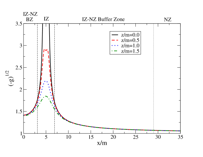
Figure 2: Global $\sqrt{-g}$ for an equal-mass BBH with equal and aligned spins $(\chi_{1},\chi_{2})=(0.9,0.9)$. The orbital separation is $b=10m$, and each BH is located on the $x$-axis at $\pm 5m$. The volume element is plotted as a function of $x$, with $y=0$ and different colors and styles correspond to different $z$-values. Since the figure is symmetric about $x=0$, we only present results around BH1. The vertical dashed and dotted lines roughly correspond to the inner and outer boundaries of the IZ/NZ transition, respectively when $z/m=0$. In the region outside the vertical dotted lines, the global metric reduces essentially to the NZ one, while in the region inside the dashed lines around $x/m=5$ the global metric reduces to the IZ one. Elsewhere, the global metric transitions between IZ and NZ metrics.

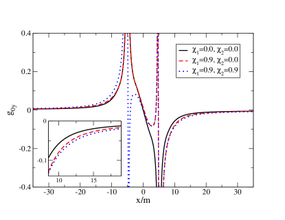
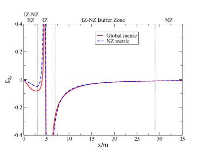
Figure 3: Left: Global $g_{0y}$ along the $x$-axis for an equal-mass BBH with different spins. The inset zooms in to the middle region of the transition from the IZ to the NZ. The IZ1 metric contributes at $\sim 2\%$ to the global metric $x/m=15$. Right: Global and NZ only $g_{0y}$ along the $x$-axis for an equal-mass BBH with spins $(\chi_{1},\chi_{2})=(0.9,0.9)$. The vertical lines are the same as in Figure 2.

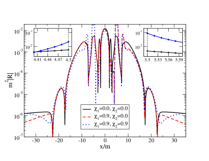
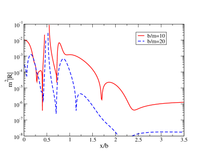
Figure 4: Left: Ricci scalar $R$ calculated with the global metric along the $x$-axis for an equal-mass BBH with orbital separation $b=10m$ but different spins. The insets zoom to a region close to BH1 for the $(\chi_{1},\chi_{2})=(0,0)$ and $(\chi_{1},\chi_{2})=(0.9,0.9)$ cases. In the insets, the dashed vertical lines denote the location of the event horizon of the IZ perturbed Kerr metric at $x=(5\pm 0.5)m$, and we stop plotting the Ricci scalar inside this region. Right: Same as left panel but for the $(\chi_{1},\chi_{2})=(0.9,0.9)$ case plotted for different orbital separations: $b=10m$ and $20m$. The $x$-axis is the field point distance, normalized to the orbital separation.

Let us now study how the matching behaves as a function of spin parameter. For this, we concentrate on the $g_{0y}$ component of the global metric, as this is one of the components most affected by different spin values. The left panel of Figure 3 plots this component along the $x$-axis, for an equal-mass BBH with different spin configurations: $(\chi_{1},\chi_{2})=(0,0)$, $(\chi_{1},\chi_{2})=(0.9,0)$, and $(\chi_{1},\chi_{2})=(0.9,0.9)$. We observe the strong spin-dependence of this metric component close to either BH (around $x/m=\pm 5$). In spite of this strong spin-dependence, we observe that the matched metric smoothly transitions between the IZs and the NZ in the BZs. Such a smooth transition is also shown on the right-panel of this figure, where we present both the global and the NZ only metrics for the $(\chi_{1},\chi_{2})=(0.9,0.9)$ case.

Finally, let us use the Ricci scalar $R$ as a measure of the accuracy to which the global metric satisfies the vacuum Einstein equations. An exact solution would of course satisfy $R=0$, but since the metrics we are employing are approximate, their associated Ricci scalars will not vanish exactly. The questions one wish to address are the following: (i) are the IZ and NZ metrics as accurate as they are supposed to be? (ii) do the transition functions introduce an error larger than that intrinsically contained in the approximate IZ and NZ metrics? Question (i) should clearly be answered in the affirmative, if the IZ and NZ metrics have been correctly calculated. Question (ii) should also be answered in the affirmative, provided the transition functions are built to satisfy the Frankenstein theorems [18].

The calculation of the Ricci scalar is not trivial due to the complexity of the IZ metric, the matching parameter and coordinate transformation, and the use of transition functions. For these reasons, we compute the Ricci on the $t=0$ spatial hypersurface through numerical methods. In doing so, we not only need the spatial derivative of the global metric, but also its time derivative. The latter requires knowledge of the time evolution of the orbital phase and frequency, summarized in the Appendix of [56], as well as the location of each BH in Eq. (15). We are using the currently-known highest PN results for the time evolution, i.e., the 3.5PN order for the non-spinning cases, and some lower order terms for the spinning cases [57]. When computing derivatives, it is of course critical to use sufficient numerical accuracy, as otherwise the Ricci scalar will be highly inaccurate, specially in the region close to the BHs.

The left panel of Figure 4 presents the Ricci scalar for different spin values, while the right panel shows this scalar for different orbital separations. First, we see that the metrics are indeed approximate solutions to the Einstein equations, as evidenced by the right panel. That is, as the orbital separation is increased, the accuracy of the metrics also increases and the Ricci scalar decreases at the expected rate. Second, we see that the transition functions have been built to satisfy the Frankenstein theorems, as they clearly do not introduce errors larger than those inherently contained in the approximate metrics. That is, the height of the humps shown in the left panel of Figure 4 for $x\in[-15,-6]\cup[-4,4]\cup[6,15]$ is of the same order as the error naturally inherent in the approximations. All of these conclusions are mildly sensitive to the spin values, demonstrating the validity of the global metric for all spins.

The extreme Kerr limit, i.e., as $\chi_{A}\to 1$, must be treated carefully. From the matching stand-point, this limit is perfectly well-behaved in a mathematical analysis sense. From a numerical standpoint, however, this limit is difficult because of excision. When evolving quantities numerically, one sometimes excises the region interior to the BH horizons, placing the excision boundary somewhere well inside the horizon. In the extreme Kerr case, the horizon shrinks and this could potentially lead to numerical problems with the excision boundary. We stress however that this is a numerical problem, and not a mathematical one with asymptotic matching.

5 Discussion

We constructed a global approximate metric that represents the binary inspiral of spinning compact objects. We split the spacetime into different zones: the IZs (close to either BH), the NZ (far from either BH but less than a GW wavelength from the center of mass) and the FZ (farther than a GW wavelength from the center of mass). In each of these zones, the spacetime is approximated through either BH perturbation theory techniques in the IZs or PN techniques in the FZs. These approximate metrics are then related to each other via asymptotic matching, which provides a coordinate and parameter transformation that renders adjacent metrics asymptotic to each other in their mutually overlapping regions of validity. Once the metrics have been asymptotically matched, they can be stitched together via certain transition functions to yield an approximate metric for non-spinning BBHs [15, 17, 19]. Here, we have extended this work to spinning BBHs where the IZ metrics are modeled through perturbed Kerr spacetimes [27] and the NZ and FZ metrics include spin-orbit terms from PN theory [24, 25, 54]. After matching, the IZ metric reduces exactly to the Kerr solution in the limit of infinite binary separation.

The approximate global metric constructed in this way is technically valid on an initial $t=0$, spatial hypersurface, but it can be extended to capture the entire temporal evolution of the binary. This evolution will be described in a future paper [29]. Of course, this time-dependent, approximate global metric is only valid provided the approximate metrics in each zone remain properly asymptotically matched, which in turn holds true if and only if a BZ exists. These overlapping regions of validity are dynamically squeezed out as the binary shrinks, and we expect the global construction to fail for sufficiently small separations, as will be studied in [29]. When the BHs are close enough, numerical relativity is required to describe the BBH spacetime.

We are planning to extend this work in multiple ways in the near future. We have here carried out asymptotic matching to lowest order, and thus, a clear extension would be to re-do this calculation but to higher order. For this to be feasible, however, one would first have to construct a vacuum-perturbed Kerr metric that includes the first time derivative of the electric and magnetic quadrupole tensors, as well as the octupole tensors. Such a metric is not available at this time, which is why we were forced to stop the matching at lowest order.

Another avenue of future work would be to explore how the dynamical approximate global metric constructed here affects certain astrophysical phenomena, such as accretion disks around a BBH. A similar study was carried out in [4], except that there non-spinning BHs were considered in the NZ metric. We expect spin-orbit coupling to be important to properly account for the total angular momentum budget of the system. For example, the spin-orbit coupling can have a dramatic effect on the inspiral rate. When the BH spins are aligned (or even partially aligned) with the orbital angular momentum, the merger is delayed, while when they are anti-aligned, the merger happens much more quickly. This effect, also know as “hangup” effect [58], is also responsible for very large kicks of the final merger remnant [59]. We also expect spins to be important to properly describe the dynamics of the individual accretion disks that may build-up around each BH during the inspiral process, specially at large separations. It would be interesting to examine what the differences are when spin is included, and whether this would lead to an electromagnetic observable precursor to BBH mergers. We will explore this in a forthcoming paper.

Appendix A Weyl Scalar for the IZ and NZ Metric

Our starting point is the IZ metric, which is given by Eqs. (YG-45) and (YG-46), where Eq. (YG-n) denotes Eq. (n) in [27]. Since the $m=0$ mode is of higher-order in the analysis of [27], it was ignored there. In this paper, however, we wish to include this mode, and thus, we derive it following the methods in [27].

First, the radial function $R_{m}$ in Eq. (YG-8) is rather simple when $m=0$:

$$R_{0} =\mbox{const.}=1\,,$$ (45)

where this constant is determined by requiring that $R_{m}\to 1$ for large radius. One can also think of this solution as that for the $m\neq 0$ modes in the Schwarzschild limit [41]. Using Eq. (YG-21) for $R_{0}$, we calculate the potential $\Psi$. The radial dependence is simply $\Delta^{2}$, and we can directly extend Eq. (YG-34) to including the $m=0$ mode. Thus, although there is a singular coefficient in the Schwarzschild limit (see Eq. (YG-33)), we may use Eq. (YG-34) for the non-spinning case. If we considered time-dependent perturbations, the reconstruction of the metric would be more complicated, as discussed for example, in [39, 40].

Next, using Eq. (YG-45) with all $(\ell,m)=(2,m)$ modes, we calculate the Weyl scalar $\psi_{0}$. One finds that $\psi_{0}=-(1/2)\psi_{0}^{\rm(orig)}$ where $\psi_{0}^{\rm(orig)}$ denotes the Weyl scalar in Eq. (YG-5). Therefore, we have obtained a relation between ${\cal E}_{kl}$, ${\cal B}_{kl}$ and $z_{R/I,m}$, as given in Eq. (22). The factor of $2$ difference arises due to a difference in normalization of $\psi_{0}$ and $\Psi$ (see, e.g., (15) in [61]). In practice, the time-time and time-space components shown in [27] and [19] are the same in the $M/R\to 0$ limit with Eq. (22).

The Weyl scalar $\psi_{0}$ can be calculated directly from the NZ metric, independently from section 3. Calculating the Weyl tensor from the NZ metric and deriving the Weyl scalar by contracting with the tetrad, we can compare it with the IZ $\psi_{0}$ in the BZ. From Eq. (21) for the NZ metric in the BZ, we have

$$\psi_{0}= \frac{3\,m_{2}}{2\,b^{3}}[(1+\cos^{2}\theta)\cos 2\phi-\sin^{2}\theta-2\,i\cos\theta\sin 2\phi]\,,$$ (46)

to leading order in $m_{2}/b$, where we are using spherical polar coordinates and we ignored any coordinate difference between the IZ and NZ. Matching then forces $z_{R,0}=2m_{2}/b^{3}$, $z_{R,\pm 2}=6m_{2}/b^{3}$ and all other coefficients to vanish. The above result is converted to ${\cal E}_{ij}=(m_{2}/b^{3})(\delta_{ij}-3\hat{x}_{i}\hat{x}_{j})$ via Eq. (22).

Appendix B Detailed Verification of the Matching Calculation

We have so far studied matching for a given set of indices in the integrability condition of Eq. (35), but now we extend this result to all indices. Using the same notations as before, and taking $(\alpha,\beta,\gamma)=(i,j,k)\neq 0$ and $\delta=0$, we now have

$$\partial_{ij}(S_{k0})_{2}-\partial_{kj}(S_{i0})_{2} =0\,,$$ (47)

which is explicitly written as

$$0= -\delta_{jk}\frac{\tilde{x}_{i}}{(R)_{0}^{3}}(\bar{\cal E}_{nm})_{0}(X^{n})_{0}(X^{m})_{0}+2\delta_{jk}\frac{1}{(R)_{0}}(\bar{\cal E}_{in})_{0}(X^{n})_{0}-2\frac{\tilde{x}_{j}\tilde{x}_{k}}{(R)_{0}^{3}}(\bar{\cal E}_{in})_{0}(X^{n})_{0}$$ (48)

$$-\delta_{ij}\frac{\tilde{x}_{k}}{(R)_{0}^{3}}(\bar{\cal E}_{nm})_{0}(X^{n})_{0}(X^{m})_{0}+3\frac{\tilde{x}_{i}\tilde{x}_{j}\tilde{x}_{k}}{(R)_{0}^{5}}(\bar{\cal E}_{nm})_{0}(X^{n})_{0}(X^{m})_{0}$$

$$-\delta_{ik}\frac{\tilde{x}_{j}}{(R)_{0}^{3}}(\bar{\cal E}_{nm})_{0}(X^{n})_{0}(X^{m})_{0}+2\delta_{ik}\frac{1}{(R)_{0}}(\bar{\cal E}_{jn})_{0}(X^{n})_{0}-2\frac{\tilde{x}_{i}\tilde{x}_{k}}{(R)_{0}^{3}}(\bar{\cal E}_{jn})_{0}(X^{n})_{0}$$

$$+2\frac{\tilde{x}_{k}}{(R)_{0}}(\bar{\cal E}_{ij})_{0}+2\delta_{ij}\frac{1}{(R)_{0}}(\bar{\cal E}_{kn})_{0}(X^{n})_{0}+2\frac{\tilde{x}_{j}}{(R)_{0}}(\bar{\cal E}_{ki})_{0}+2\frac{\tilde{x}_{i}}{(R)_{0}}(\bar{\cal E}_{kj})_{0}$$

$$-2\frac{\tilde{x}_{i}\tilde{x}_{j}}{(R)_{0}^{3}}(\bar{\cal E}_{kn})_{0}(X^{n})_{0}-(i\leftrightarrow k)\,,$$

where $\tilde{x}^{i}=(X^{i})_{0}$. This equation is trivially consistent, and thus, it provides no additional information about $(\bar{\cal E}_{ij})_{0}$.

The last set of indices to verify is $(\alpha,\beta,\gamma,\delta)=(i,j,k,l)\neq 0$. The integrability condition becomes

$$\partial_{ij}(S_{kl})_{2}+\partial_{kl}(S_{ij})_{2}-\partial_{il}(S_{kj})_{2}-\partial_{kj}(S_{il})_{2} =0\,.$$ (49)

As before, this equation can be divided into a polynomial and a non-polynomial part. The non polynomial part gives again $(M_{1})_{0}=m_{1}$, and once more the constant and first order pieces give trivial relations. The quadrupolar part gives

$$0= (6\hat{x}_{i}\hat{x}_{j}-2\delta_{ij})\delta_{kl}+\frac{2}{3}(\bar{\cal E}_{ij})_{0}\delta_{kl}+\frac{4}{3}(\bar{\cal E}_{kl})_{0}\delta_{ij}+(6\hat{x}_{k}\hat{x}_{l}-2\delta_{kl})\delta_{ij}+\frac{2}{3}(\bar{\cal E}_{kl})_{0}\delta_{ij}$$ (50)

$$+\frac{4}{3}(\bar{\cal E}_{ij})_{0}\delta_{kl}-(6\hat{x}_{i}\hat{x}_{l}-2\delta_{il})\delta_{kj}+\frac{2}{3}(\bar{\cal E}_{il})_{0}\delta_{kj}+\frac{4}{3}(\bar{\cal E}_{kj})_{0}\delta_{il}+\frac{4}{3}(\bar{\cal E}_{il})_{0}\delta_{kj}$$

$$-(6\hat{x}_{k}\hat{x}_{j}-2\delta_{kj})\delta_{il}+\frac{2}{3}(\bar{\cal E}_{kj})_{0}\delta_{il}\,,$$

which once again leads to $(\bar{\cal E}_{ij})_{0}=\delta_{ij}-3\hat{x}_{i}\hat{x}_{j}$.

Let us now focus on the coordinate transformation. We need to solve

$$2(A_{(\alpha\beta)})_{2} =(g^{{\mbox{\tiny NZ}}}_{\alpha\beta})_{2}-(g^{{\mbox{\tiny IZ}}}_{\alpha\beta})_{2}-(F_{\alpha}{}^{\gamma})_{1}(F_{\beta\gamma})_{1}\,,$$ (51)

or more explicitly, using the expression for $(\bar{\cal E}_{kj})_{0}$,

$$2(A_{(\alpha\beta)})_{2}= \biggl{[}(2-\frac{2}{b}\tilde{x})\Delta_{\alpha\beta}-(F_{\alpha}{}^{\gamma})_{1}(F_{\beta\gamma})_{1}\biggr{]}-\biggl{[}\delta_{\alpha}^{i}\delta_{\beta}^{j}\frac{2}{b^{2}}\Bigl{(}(\tilde{x}^{k}\tilde{x}_{k})\hat{x}_{i}\hat{x}_{j}-\tilde{x}^{2}\delta_{ij}\Bigr{)}\biggr{]}$$ (52)

$$+\biggl{[}(\delta_{\alpha}^{i}\hat{t}_{\beta}+\delta_{\beta}^{i}\hat{t}_{\alpha})\frac{1}{3b^{2}}\Bigl{(}3\tilde{x}_{i}\sqrt{\tilde{x}^{k}\tilde{x}_{k}}-3\frac{\tilde{x}_{i}}{(R)_{0}}\tilde{x}^{2}-6(R)_{0}\hat{x}_{i}\tilde{x}\Bigr{)}\biggr{]}\,,$$

where we used the abbreviation $\tilde{x}=\tilde{x}^{k}\hat{x}_{k}=\tilde{x}^{\alpha}\hat{x}_{\alpha}$ because $\hat{x}_{0}=0$. The solution to this equation is obtained by adding the general flat solution to a particular solution. The general solution is then

$$(X_{\alpha})_{2,g} =(F_{\alpha\beta})_{2}\tilde{x}^{\beta}+(C_{\alpha})_{2}\,.$$ (53)

The first bracket in Eq. (52) is the same as the one found in [19] during second-order matching. The particular solution for this term is

$$(X_{\alpha})_{2,p1}= \Bigl{[}1-\frac{\tilde{x}}{b}\Bigr{]}\Delta_{\alpha\beta}\tilde{x}^{\beta}+\frac{\Delta_{\gamma\delta}\tilde{x}^{\gamma}\tilde{x}^{\delta}}{2b}\hat{x}_{\alpha}-\frac{1}{2}(F_{\alpha}{}^{\gamma})_{1}(F_{\delta\gamma})_{1}\tilde{x}^{\delta}\,.$$ (54)

For the second bracket, a particular solution is

$$(X_{\alpha})_{2,p2} =-\frac{1}{b^{2}}\Bigl{[}(\tilde{x}^{k}\tilde{x}_{k})\tilde{x}\hat{x}_{i}-\tilde{x}^{2}\tilde{x}_{i}\Bigr{]}\delta_{\alpha}^{i}\,.$$ (55)

For the third bracket, we can take the particular solution

$$(X_{\alpha})_{2,p3} =\frac{1}{3b^{2}}\Bigl{[}(\tilde{x}^{k}\tilde{x}_{k})^{3/2}-3\tilde{x}^{2}\sqrt{\tilde{x}^{k}\tilde{x}_{k}}\Bigr{]}\hat{t}_{\alpha}\,.$$ (56)

Combining the general and particular solutions, we obtain the expression in Eq. (40).

Appendix C Transition function

The construction of a smooth approximate global metric requires the stitching of the asymptotically matched IZ, NZ and FZ metrics through certain transition functions, $f_{\rm far}$, $f_{\rm near}$, $f_{{\rm inner},1}$ and $f_{{\rm inner},2}$:

$$g_{\mu\nu}= (1-f_{\rm far})\Bigl{\{}f_{\rm near}\bigl{[}f_{{\rm inner},1}\,g_{\mu\nu}^{{\mbox{\tiny NZ}}}+(1-f_{{\rm inner},1})\,g_{\mu\nu}^{\rm(IZ1)}\bigr{]}$$ (57)

$$+(1-f_{\rm near})\bigl{[}f_{{\rm inner},2}\,g_{\mu\nu}^{{\mbox{\tiny NZ}}}+(1-f_{{\rm inner},2})\,g_{\mu\nu}^{\rm(IZ2)}\bigr{]}\Bigr{\}}+f_{\rm far}\,g_{\mu\nu}^{{\mbox{\tiny FZ}}}\,.$$

These transition functions can be modeled via

$$f(r,\,r_{0},\,w,\,q,\,s)=\cases{0,&$r\leq r_{0}$,\\ \frac{1}{2}\left\{1+\tanh\left[\frac{s}{\pi}\left(\chi(r,\,r_{0},\,w)-\frac{q^{2}}{\chi(r,\,r_{0},\,w)}\right)\right]\right\},&\\ \hskip 25.60747ptr_{0}<r<r_{0}+w,&\\ 1,&$r\geq r_{0}+w$,\\ }$$ (58)

where $\chi(r,r_{0},w)=\tan[\pi(r-r_{0})/(2w)]$, and $r_{0}$, $w$, $q$ and $s$ are parameters. Such a transition function has been greatly discussed in [15, 17, 19] and it satisfies the Frankenstein conditions of [18].

The transition functions are chosen with the following parameters.

$$f_{\rm far} =f(r,\,\lambda/5,\,\lambda,\,1,\,1.4)\,,$$ (59)

$$f_{\rm near} =f(x,\,2.2\,m_{2}-\frac{m_{1}b}{m},\,b-2.2\,m,\,1,\,2.5)\,,$$ (60)

$$f_{{\rm inner},A} =f(r_{A},\,0.4\,r_{A}^{T},\,3.5\,(mb^{4})^{1/5},\,0.2,\,b/m)\,.$$ (61)

Here, $r$ is the distance from the binary’s center-of-mass to the field point. The parameter $s=1.4$ has been discussed in [29] and it is different from that of [19], which reduces the magnitude of the first radial derivative. The quantity $\lambda=\pi\sqrt{b^{3}/M}$ is the gravitational wavelength in the Newtonian limit. We assume that the BHs are initially located on the $x$-axis.

The transition function $f_{{\rm inner},A}$ is somewhat different from that chosen in [19]. This is because we match here to a different order than in the latter paper. In particular, the “transition radius” $r_{A}^{T}$, where the leading-order uncontrolled remainder of adjacent zones becomes comparable, is here given by

$$\left(\frac{m}{b}\right)\left(\frac{r_{A}^{T}}{b}\right)^{3} =\left(\frac{m_{A}}{r_{A}^{T}}\right)^{2}\,,$$ (62)

where the left- and right-hand sides correspond to the IZ and NZ remainders, respectively. The quantity $(r_{A}^{T}/b)^{3}$ in the IZ remainder arises due to ignorance in the octupole contribution to the BH perturbation. In the NZ, the remainder is $(m_{A}/r_{A}^{T})^{2}$. The transition radius is thus $r_{A}^{T}=(m_{A}^{2}b^{4}/m)^{1/5}$, which is the same as in [17]. The numerical coefficients in $f_{{\rm inner},A}$, $0.4$ and $3.5$, are also from [17], and the $(mb^{4})^{1/5}$ dependence is obtained by setting $m_{A}=m$ in $r_{A}^{T}$, as studied in [19].

Appendix D Higher Order Metrics

Ref. [19] constructed a 2.5PN, non-spinning NZ metric following [23]. In this paper, we have included certain higher PN order terms, when numerically calculating certain quantities in section 4.

For the NZ metric, this higher-order extension is achieved by adding the following terms, $\delta g_{\mu\nu}^{{\mbox{\tiny NZ}}}$ to the 1.5PN order metric of Eq. (8):

$$\delta g_{00}^{{\mbox{\tiny NZ}}}=\delta g_{00}^{{\mbox{\tiny NZ}},(6)}+\delta g_{00}^{{\mbox{\tiny NZ}},(7)}+{\cal{O}}(v^{8})\,,$$

$$\delta g_{0i}^{{\mbox{\tiny NZ}}}=\delta g_{0i}^{{\mbox{\tiny NZ}},(5)}+\delta g_{0i}^{{\mbox{\tiny NZ}},(6)}+{\cal{O}}(v^{7})\,,$$

$$\delta g_{ij}^{{\mbox{\tiny NZ}}}=\delta g_{ij}^{{\mbox{\tiny NZ}},(4)}+\delta g_{0i}^{{\mbox{\tiny NZ}},(5)}+{\cal{O}}(v^{6})\,.$$ (63)

For example, $\delta g_{0i}^{{\mbox{\tiny NZ}},(5)}$ and $\delta g_{ij}^{{\mbox{\tiny NZ}},(4)}$ are explicitly given by

$$\delta g_{0i}^{{\mbox{\tiny NZ}},(5)}= -n_{1}^{i}\Biggl{[}\frac{m_{1}^{2}}{r_{1}^{2}}(\mathbf{n}_{1}\cdot\mathbf{v}_{1})+\frac{m_{1}m_{2}}{\tilde{S}^{2}}\bigl{\{}16(\mathbf{n}_{12}\cdot\mathbf{v}_{1})-12(\mathbf{n}_{12}\cdot\mathbf{v}_{2})+16(\mathbf{n}_{2}\cdot\mathbf{v}_{1})$$

$$-12(\mathbf{n}_{2}\cdot\mathbf{v}_{2})\bigr{\}}\Biggr{]}-n_{12}^{i}m_{1}m_{2}\Biggl{[}6(\mathbf{n}_{12}\cdot\mathbf{v}_{12})\frac{r_{1}}{b^{3}}+4(\mathbf{n}_{1}\cdot\mathbf{v}_{1})\frac{1}{b^{2}}-12(\mathbf{n}_{1}\cdot\mathbf{v}_{1})\frac{1}{\tilde{S}^{2}}$$

$$+16(\mathbf{n}_{1}\cdot\mathbf{v}_{2})\frac{1}{\tilde{S}^{2}}-4(\mathbf{n}_{12}\cdot\mathbf{v}_{1})\frac{1}{\tilde{S}}\Bigl{(}\frac{1}{\tilde{S}}+\frac{1}{b}\Bigr{)}\Biggr{]}+v_{1}^{i}\Biggl{[}\frac{m_{1}}{r_{1}}(2(\mathbf{n}_{1}\cdot\mathbf{v}_{1})^{2}-4v_{1}^{2})+\frac{m_{1}^{2}}{r_{1}^{2}}$$

$$+m_{1}m_{2}\Bigl{(}\frac{3r_{1}}{b^{3}}-\frac{2r_{2}}{b^{3}}\Bigr{)}-m_{1}m_{2}\Bigl{(}\frac{r_{2}^{2}}{r_{1}b^{3}}+\frac{3}{r_{1}b}-\frac{8}{r_{2}b}+\frac{4}{b\tilde{S}}\Bigr{)}\Biggr{]}+(1\leftrightarrow 2)\,,$$

$$\delta g_{ij}^{{\mbox{\tiny NZ}},(4)}= \Biggl{[}-\frac{m_{1}}{r_{1}}(\mathbf{n}_{1}\cdot\mathbf{v}_{1})^{2}+\frac{m_{1}^{2}}{r_{1}^{2}}+m_{1}m_{2}\Bigl{(}\frac{2}{r_{1}r_{2}}-\frac{r_{1}}{2b^{3}}+\frac{r_{1}^{2}}{2r_{2}b^{3}}-\frac{5}{2r_{1}b}+\frac{4}{b\tilde{S}}\Bigr{)}\Biggr{]}\delta_{ij}$$ (64)

$$+4\frac{m_{1}}{r_{1}}v_{1}^{i}v_{1}^{j}+\frac{m_{1}^{2}}{r_{1}^{2}}n_{1}^{i}n_{1}^{j}-4m_{1}m_{2}n_{12}^{i}n_{12}^{j}\left(\frac{1}{\tilde{S}^{2}}+\frac{1}{b\tilde{S}}\right)$$

$$+4\frac{m_{1}m_{2}}{\tilde{S}^{2}}(n_{1}^{(i}n_{2}^{j)}+2n_{1}^{(i}n_{12}^{j)})+(1\leftrightarrow 2)\,.$$

In the above equations, we have introduced the notation

$$\tilde{S}=r_{1}+r_{2}+b\,,$$ (65)

where the quantity $\tilde{S}$ is a distance parameter that is not to be confused with the magnitude of the spin angular momentum $s_{1}$ or $s_{2}$. The other higher-order pieces can be obtained up from Eq. (7.2) in [23]; for example, $\delta g_{00}^{{\mbox{\tiny NZ}},(6)}$ is a contribution of ${\cal{O}}(1/c^{6})$ that can be found in Eq. (7.2a) of [23].

For the FZ metric, the higher-order extension is obtained by replacing Eq. (12) with

$$g_{00}^{{\mbox{\tiny FZ}}}=-\left[1-\frac{1}{2}\,h^{00}_{{\mbox{\tiny FZ}}}+\frac{3}{8}\,\left(h_{{\mbox{\tiny FZ}}}^{00}\right)^{2}\right]+\frac{1}{2}\,h_{{\mbox{\tiny FZ}}}^{kk}\,,$$

$$g_{0k}^{{\mbox{\tiny FZ}}}=-\left[1-\frac{1}{2}\,h_{{\mbox{\tiny FZ}}}^{00}\right]h_{{\mbox{\tiny FZ}}}^{0k}\,,$$

$$g_{kl}^{{\mbox{\tiny FZ}}}=\left[1+\frac{1}{2}\,h_{{\mbox{\tiny FZ}}}^{00}-\frac{1}{8}\,\left(h_{{\mbox{\tiny FZ}}}^{00}\right)^{2}-\frac{1}{2}h_{{\mbox{\tiny FZ}}}^{pp}\right]\delta^{kl}+h_{{\mbox{\tiny FZ}}}^{kl}\,,$$ (66)

with ${\cal{O}}(v^{6})$ remainders. The metric potentials $h_{{\mbox{\tiny FZ}}}^{\mu\nu}$ must also extended to higher-order via

$$h_{{\mbox{\tiny FZ}}}^{00}=4\,\frac{{\cal{I}}}{r}+2\,\partial_{kl}\left[\frac{{\cal{I}}^{kl}(u)}{r}\right]-\frac{2}{3}\,\partial_{klm}\left[\frac{{\cal{I}}^{klm}(u)}{r}\right]+7\,\frac{{\cal{I}}^{2}}{r^{2}}\,,$$

$$h_{{\mbox{\tiny FZ}}}^{0k}=-2\,\partial_{l}\left[\frac{\dot{\cal{I}}^{kl}(u)}{r}\right]+2\,\epsilon^{lkp}\frac{n^{l}{\cal{J}}^{p}}{r^{2}}+\frac{2}{3}\,\partial_{lp}\left[\frac{\dot{\cal{I}}^{klp}(u)}{r}\right]+\frac{4}{3}\,\epsilon^{lkp}\partial_{ls}\left[\frac{{\cal{J}}^{ps}(u)}{r}\right]\,,$$

$$h_{{\mbox{\tiny FZ}}}^{kl}=2\,\frac{\ddot{\cal{I}}^{kl}(u)}{r}-\frac{2}{3}\,\partial_{p}\left[\frac{\ddot{\cal{I}}^{klp}(u)}{r}\right]-\frac{8}{3}\,\epsilon^{ps(k|}\partial_{s}\left[\frac{\dot{\cal{J}}^{p|l)}(u)}{r}\right]+\frac{{\cal{I}}^{2}}{r^{2}}\hat{n}^{k}\hat{n}^{l}\,,$$ (67)

again with ${\cal{O}}(v^{6})$ remainders.

References

References

- [1] Pretorius F 2005 Phys. Rev. Lett. 95 121101 (Preprint gr-qc/0507014)
- [2] Campanelli M, Lousto C, Marronetti P and Zlochower Y 2006 Phys. Rev. Lett. 96 111101 (Preprint gr-qc/0511048)
- [3] Baker J G, Centrella J, Choi D I, Koppitz M and van Meter J 2006 Phys. Rev. Lett. 96 111102 (Preprint gr-qc/0511103)
- [4] Noble S C, Mundim B C, Nakano H, Krolik J H, Campanelli M, Zlochower Y and Yunes N 2012 Astrophys. J. 755 51 (Preprint 1204.1073)
- [5] Blanchet L 2006 Living Rev. Rel. 9 4 (Preprint gr-qc/0202016)
- [6] Thorne K 1980 Rev. Mod. Phys. 52 299–339
- [7] Poisson E 2005 Phys. Rev. Lett. 94 161103 (Preprint gr-qc/0501032)
- [8] Taylor S and Poisson E 2008 Phys. Rev. D78 084016 (Preprint 0806.3052)
- [9] Comeau S and Poisson E 2009 Phys. Rev. D80 087501 (Preprint 0908.4518)
- [10] Poisson E and Vlasov I 2010 Phys. Rev. D81 024029 (Preprint 0910.4311)
- [11] Vega I, Poisson E and Massey R 2011 Class. Quant. Grav. 28 175006 (Preprint 1106.0510)
- [12] Poisson E, Pound A and Vega I 2011 Living Rev. Rel. 14 7 (Preprint 1102.0529)
- [13] Alvi K 2000 Phys. Rev. D61 124013 (Preprint gr-qc/9912113)
- [14] Alvi K 2003 Phys. Rev. D67 104006 (Preprint gr-qc/0302061)
- [15] Yunes N, Tichy W, Owen B J and Bruegmann B 2006 Phys. Rev. D74 104011 (Preprint gr-qc/0503011)
- [16] Bender C M and Orszag S A 1999 Advanced mathematical methods for scientists and engineers 1, Asymptotic methods and perturbation theory (New York: Springer)
- [17] Yunes N and Tichy W 2006 Phys. Rev. D74 064013 (Preprint gr-qc/0601046)
- [18] Yunes N 2007 Class. Quant. Grav. 24 4313–4336 (Preprint gr-qc/0611128)
- [19] Johnson-McDaniel N K, Yunes N, Tichy W and Owen B J 2009 Phys. Rev. D80 124039 (Preprint 0907.0891)
- [20] Reifenberger G and Tichy W 2012 (Preprint 1205.5502)
- [21] Chu T 2012 Numerical simulations of black-hole spacetimes Ph.D. thesis California Institute of Technology Pasadena, CA 91125, USA URL http://thesis.library.caltech.edu/6556/
- [22] Owen B J, Tagoshi H and Ohashi A 1998 Phys. Rev. D57 6168–6175 (Preprint gr-qc/9710134)
- [23] Blanchet L, Faye G and Ponsot B 1998 Phys. Rev. D58 124002 (Preprint gr-qc/9804079)
- [24] Tagoshi H, Ohashi A and Owen B J 2001 Phys. Rev. D63 044006 (Preprint gr-qc/0010014)
- [25] Faye G, Blanchet L and Buonanno A 2006 Phys. Rev. D74 104033 (Preprint gr-qc/0605139)
- [26] Blanchet L, Buonanno A and Faye G 2006 Phys. Rev. D74 104034 (Preprint gr-qc/0605140)
- [27] Yunes N and González J A 2006 Phys. Rev. D73 024010 (Preprint gr-qc/0510076)
- [28] Cook G B and Scheel M A 1997 Phys. Rev. D56 4775–4781
- [29] Mundim B C et al. In preparation
- [30] Misner C W, Thorne K and Wheeler J A 1973 Gravitation (San Francisco: W. H. Freeman & Co.)
- [31] Detweiler S L 2005 Class. Quant. Grav. 22 S681–S716 (Preprint gr-qc/0501004)
- [32] Regge T and Wheeler J A 1957 Phys. Rev. 108 1063–1069
- [33] Zerilli F J 1970 Phys. Rev. D2 2141–2160
- [34] Moncrief V 1974 Annals Phys. 88 323–342
- [35] Teukolsky S A 1973 Astrophys. J. 185 635–647
- [36] Chrzanowski P L 1975 Phys. Rev. D11 2042–2062
- [37] Wald R M 1978 Phys. Rev. Lett. 41 203–206
- [38] Kegeles L S and Cohen J M 1979 Phys. Rev. D19 1641–1664
- [39] Lousto C O and Whiting B F 2002 Phys. Rev. D66 024026 (Preprint gr-qc/0203061)
- [40] Ori A 2003 Phys. Rev. D67 124010 (Preprint gr-qc/0207045)
- [41] Poisson E 2004 Phys. Rev. D70 084044 (Preprint gr-qc/0407050)
- [42] Abe M, Ichinose S and Nakanishi N 1987 Prog. Theor. Phys. 78 1186
- [43] Ruiz E 1986 Gen. Rel. Grav. 18 805–811
- [44] Aguirregabiria J M, Bel L, Martin J, Molina A and Ruiz E 2001 Gen. Rel. Grav. 33 1809–1838 (Preprint gr-qc/0104019)
- [45] Cook G B 2000 Living Rev. Rel. 3 5 (Preprint gr-qc/0007085)
- [46] Hergt S and Schaefer G 2008 Phys. Rev. D77 104001 (Preprint 0712.1515)
- [47] Sopuerta C F and Yunes N 2011 Phys. Rev. D84 124060 (Preprint 1109.0572)
- [48] Will C M and Wiseman A G 1996 Phys. Rev. D54 4813–4848 (Preprint gr-qc/9608012)
- [49] Pati M E and Will C M 2000 Phys. Rev. D62 124015 (Preprint gr-qc/0007087)
- [50] Pati M E and Will C M 2002 Phys. Rev. D65 104008 (Preprint gr-qc/0201001)
- [51] Blanchet L, Damour T and Iyer B R 1995 Phys. Rev. D51 5360 (Preprint gr-qc/9501029)
- [52] Blanchet L 1995 Phys. Rev. D51 2559–2583 (Preprint gr-qc/9501030)
- [53] Blanchet L 1996 Phys. Rev. D54 1417–1438 (Preprint gr-qc/9603048)
- [54] Will C M 2005 Phys. Rev. D71 084027 (Preprint gr-qc/0502039)
- [55] Kidder L E 1995 Phys. Rev. D52 821–847 (Preprint gr-qc/9506022)
- [56] Ajith P, Boyle M, Brown D A, Fairhurst S, Hannam M, Hinder I, Husa S, Krishnan B, Mercer R A, Ohme F, Ott C D, Read J S, Santamaria L and Whelan J T 2007 (Preprint 0709.0093)
- [57] Ajith P, Boyle M, Brown D A, Brugmann B, Buchman L T et al. 2012 Class. Quant. Grav. 29 124001 (Preprint 1201.5319)
- [58] Campanelli M, Lousto C and Zlochower Y 2006 Phys. Rev. D74 041501 (Preprint gr-qc/0604012)
- [59] Lousto C O and Zlochower Y 2011 Phys. Rev. Lett. 107 231102 (Preprint 1108.2009)
- [60] GRTensorII this is a package which runs within Maple but distinct from packages distributed with Maple. It is distributed freely on the World-Wide-Web from the address: http://grtensor.org
- [61] Whiting B F and Price L R 2005 Class. Quant. Grav. 22 S589–S604