The completeness of quantum theory for predicting measurement outcomes

Abstract

The predictions that quantum theory makes about the outcomes of measurements are generally probabilistic. This has raised the question whether quantum theory can be considered complete, or whether there could exist alternative theories that provide improved predictions. Here we review recent work that considers arbitrary alternative theories, constrained only by the requirement that they are compatible with a notion of “free choice” (defined with respect to a natural causal order). It is shown that quantum theory is “maximally informative”, i.e., there is no other compatible theory that gives improved predictions. Furthermore, any alternative maximally informative theory is necessarily equivalent to quantum theory. This means that the state a system has in such a theory is in one-to-one correspondence with its quantum-mechanical state (the wave function). In this sense, quantum theory is complete.

I Introduction

In this

Chapter

we look at the question of whether quantum theory is optimal in terms of the predictions it makes about measurement outcomes, or whether, instead, there could exist an alternative theory with improved predictive power. This was much debated in the early days of quantum theory, when many eminent physicists supported the view that quantum theory will eventually be replaced by a deeper underlying theory. Our aim will be to show that no alternative theory can extend the predictive power of quantum theory, and hence that, in this sense, quantum theory is complete.

Before turning to this question, it is worth reflecting on why one might think that quantum theory may not be optimally predictive. A key factor is that the theory is probabilistic. This is in stark contrast with classical theory, which is deterministic at a fundamental level. Even in classical theory there are scenarios where we may assign probabilities to various events, for example when making a weather forecast. However, this isn’t in conflict with our belief in underlying determinism, but, instead, the fact that we assign probabilities simply reflects a lack of knowledge (about the precise value of certain physical quantities) when making the prediction. By analogy, we might imagine that even if we know the quantum state of a system before measurement (i.e., its wave function), we are also in a position of incomplete knowledge, and that additional knowledge might be provided in a higher theory.

A further argument for incompleteness was given by Einstein, Podolsky and Rosen (EPR) EPR . They argued that whenever the outcome of an experiment can be predicted with certainty, there should be a counterpart in the theory representing its value. They then consider measurements on a maximally entangled pair. In this scenario, the outcome of any measurement on one member of the pair can be perfectly predicted given access to the other member. Since the particles can be far apart, a measurement on one shouldn’t, say EPR, affect the other in any way. They hence argue that there should be parts of the theory allowing these perfect predictions and, hence, that the quantum description is incomplete.

Following EPR, one might hope that quantum theory can be explained in terms of an underlying deterministic theory. Such a view was put into doubt by the Bell-Kochen-Specker theorem, independently discovered by Kochen and Specker KS and by Bell Bell_KS , who showed that an underlying deterministic theory is not possible if one demands non-contextuality and freedom of choice. (A non-contextual theory is one in which the probability of a particular measurement outcome occurring depends only on the projector associated with that outcome, and not on the entire set of projectors that specify the measurement according to quantum theory.) Furthermore it was also shown by Bell Bell that there cannot be an underlying theory that is compatible with local causality (we will explain this in more detail in Section V). It is also worth noting that an assumption about locality can be seen as a physical means of justifying certain non-contextuality conditions.

In this

Chapter

, we consider arbitrary alternative theories and ask whether they could have more predictive power than quantum theory. We remark that this question is different from those asked by Kochen and Specker and by Bell, whose goal was to rule out theories with certain specific properties such as non-contextuality or local causality. In this work, we do not demand any of these properties. The only assumption we make about a theory is that it is compatible with a notion of free choice (defined with respect to a natural causal order—see later). Roughly, the freedom of choice assumption demands that the theory can be applied to a setting where an experimenter makes certain choices independently of certain pre-existing parameters. It is worth noting that quantum theory is compatible with this assumption, as we would expect, since it is a reasonable theory. We also remark that such an assumption is necessary for Kochen and Specker’s as well as for Bell’s arguments.

As a toy example of an alternative theory that enables improved predictions over those of quantum theory, but which may still be probabilistic, one might imagine that the quantum state is supplemented by an additional parameter $Z$. When measuring one half of a maximally entangled pair of qubits, it could be that if $Z=0$ the extended theory assigns outcome $0$ with probability $3/4$, and outcome $1$ with probability $1/4$, while, if $Z=1$, the extended theory assigns outcome $0$ with probability $1/4$, and outcome $1$ with probability $3/4$. The extended theory would thus provide more information than quantum theory, which predicts that both outcomes occur with probability $1/2$. Furthermore, if $Z$ is uniformly distributed, the quantum predictions are recovered when $Z$ is unknown (and hence the extended theory is compatible with quantum theory).

This particular example is rather artificial and its purpose is merely to illustrate that—in principle—a theory that is more informative than quantum theory is conceivable. However, there are historical precedents of this type, for instance related to the problem of determining the mass of chemical elements. Take, as an example, the atomic mass of chlorine. Before the discovery of isotopes, its atomic mass was thought to be $35.5$, and the standard measurement techniques of the time confirmed it as such. However, it was later discovered that chlorine in fact naturally occurs as two isotopes with atomic masses $35$ and $37$ (in approximate ratio $3:1$). By introducing isotopes, the theory was extended in such a way that the mass of an individual atom could be better predicted. Note that the predictions made before the discovery of isotopes were not incorrect, but are simply the natural ones to make without knowledge of the different isotopes (and hence the new theory is compatible with the old one).

Returning to quantum theory, various alternatives, motivated more physically than our earlier toy example, have been proposed in the past, some of which we will review later (see Section V). Similarly to quantum theory, these alternatives provide rules to compute predictions for future measurement outcomes, based on certain (additional) parameters.

The aim of this

Chapter

is to explain recent results relating the predictive power of quantum theory to that of possible alternative theories CR_ext ; CR_wavefn . For this, we first need to specify what we mean by “quantum theory” and by “alternative theories”, and how they can be compared (Section III). The central requirement we impose on any alternative theory is that it be compatible with a notion of “free choice”. This means that the theory can be applied consistently in scenarios where measurements are chosen independently of certain other events (Section IV). We then discuss the implications of some existing results to our main question. These impose constraints on any alternative theory that is compatible with quantum theory; for instance, no such theory can be locally deterministic (Section V). The last sections are then devoted to the recent, more general, results. A central claim is that no alternative theory that is compatible with quantum theory can improve the predictions of quantum theory (Sections VI and VII). Furthermore, if such an alternative theory is also at least as informative as quantum theory, then it is necessarily equivalent to quantum theory (Section VIII). In this sense, quantum theory is complete. We conclude with a discussion of how these results relate to known hidden-variable theories, in particular the de Broglie-Bohm theory, and mention some applications (Section IX).

II Preliminaries

II.1 Notation

On a technical level, the main results presented in this

Chapter

are theorems about random variables (RVs) whose (joint) probability distribution satisfies certain assumptions. We will only use RVs with discrete range. In the following we introduce our notation for such RVs and their distributions.

We usually use upper case letters to denote RVs, while lower case letters specify particular values they can take. Thus, $X=x$ means that the RV $X$ takes the value $x$. We write $P_{X}$ to denote the probability distribution of the RV $X$, with $P_{X}(x)$ being the probability that $X=x$. For two RVs, $X$ and $Y$, $P_{XY}$ represents their joint distribution. We also use $P_{X|Y}:=P_{XY}/P_{Y}$ to represent the conditional distribution of $X$ given $Y$. This is defined for all $y$ such that $P_{Y}(y)>0$. For any such $y$, we write $P_{X|Y=y}:=P_{X|Y}(\cdot,y)$ to denote the distribution of the RV $X$ conditioned on $Y=y$. We often abbreviate this distribution to $P_{X|y}$. We also use $P(X=Y)$ to denote the probability that the RVs $X$ and $Y$ have equal values, i.e. $P(X=Y):=\sum_{x}P_{XY}(x,x)$ and, likewise, $P(X\neq Y):=1-P(X=Y)$.

II.2 Distance between probability distributions

Our technical argument uses the variational distance to quantify the closeness of two probability distributions. For two distributions, $P_{X}$ and $Q_{X}$, it is defined by

$$D(P_{X},Q_{X}):=\frac{1}{2}\sum_{x}|P_{X}(x)-Q_{X}(x)|\,.$$

This measure is connected to the distinguishability of the two distributions. Specifically, suppose we have a black box that samples either from $P_{X}$ or $Q_{X}$. Then, given one sample, the maximum probability of successfully guessing whether the sample has been generated from $P_{X}$ or $Q_{X}$ equals $\frac{1}{2}(1+D(P_{X},Q_{X}))$. Thus, if two distributions are close in variational distance, they are virtually indistinguishable. Appendix A summarizes some properties of $D(\cdot,\cdot)$ that are used in this work.

II.3 Measuring correlations

A useful approach towards characterizing alternative theories is to consider the correlations (between the outcomes of two distant measurements) that can be reproduced by a given theory. The strength of these correlations may then, for instance, be compared to those occurring in quantum theory. To quantify correlations, we use a measure that has been proposed by Pearle Pearle and, independently, by Braunstein and Caves BC , based on earlier work by Clauser, Horne, Shimony, and Holt CHSH .

The correlation measure is tailored to a specific bipartite setup where measurements are carried out at two separate locations. One of the measurements is specified by a parameter $A$ and has outcome $X$. The other is specified by a parameter $B$ and has outcome $Y$. It is furthermore assumed that the outcomes $X$ and $Y$ take values from the binary set $\{0,1\}$ and that the parameters $A$ and $B$ are labelled by elements from the sets $\{0,2,\ldots,2N-2\}=:\mathcal{A}_{N}$ and $\{1,3,\ldots,2N-1\}=:\mathcal{B}_{N}$, respectively, where $N$ is an integer. The correlation measure, in the following denoted by $I_{N}$, is then defined by

$$I_{N}(P_{XY|AB}):=P(X=Y|A=0,B=2N-1)+$$

$$\sum_{\genfrac{}{}{0.0pt}{}{a\in\mathcal{A}_{N},\,b\in\mathcal{B}_{N}}{|a-b|=1}}\!\!\!\!P(X\neq Y|A=a,B=b)\,,$$

and depicted in Figure 1. Note that the measure only depends on the conditional distribution $P_{XY|AB}$, and that stronger correlations have a lower value of $I_{N}$.

Figure 1: Illustration of the terms in the correlation measure $I_{N}$. This measure is defined as the sum of the probabilities of obtaining opposite outcomes when measuring two subsystems in neighbouring bases (depicted with the solid lines), and of obtaining the same outcomes for $a=0$, $b=2N-1$ (depicted with the dashed line).

We will be particularly interested in the correlations that quantum theory predicts for measurements on two maximally entangled two-level systems. To specify these correlations, define

$$\left|\psi_{2}\right\rangle:=\frac{1}{\sqrt{2}}(\left|\uparrow\uparrow\right\rangle+\left|\downarrow\downarrow\right\rangle)\ ,$$

where $\{\left|\uparrow\right\rangle,\left|\downarrow\right\rangle\}$ is an orthonormal basis. Furthermore, let $\left|\theta\right\rangle=\cos\frac{\theta}{2}\left|\uparrow\right\rangle+\sin\frac{\theta}{2}\left|\downarrow\right\rangle$, and take $E_{x}^{a}$ to be the projector onto $\left|(\frac{a}{2N}+x)\pi\right\rangle$ and, likewise, $F_{y}^{b}$ to be the projector onto $\left|(\frac{b}{2N}+y)\pi\right\rangle$, as shown in Figure 2. We then define $P^{N}_{XY|AB\psi_{2}}$ as the conditional distribution of the outcomes of two separate quantum measurements, specified by $\{E_{x}^{a}\}_{x}$ and $\{F_{y}^{b}\}_{y}$, respectively, applied to two separate subsystems with joint state $\left|\psi_{2}\right\rangle$, i.e.,

$$P^{N}_{XY|ab\psi_{2}}(x,y):=\left\langle\psi_{2}\right|E_{x}^{a}\otimes F_{y}^{b}\left|\psi_{2}\right\rangle\ .$$

It is easy to verify that the correlation strength, quantified with the above correlation measure, $I_{N}$, equals

$$I_{N}(P^{N}_{XY|AB\psi_{2}})=2N\sin^{2}\frac{\pi}{4N}\leq\frac{\pi^{2}}{8N}\ .$$ (1)

Figure 2: Depiction of the measurements used to achieve the quantum value of the correlation measure $I_{N}$. The circle represents the $\{\left|\uparrow\right\rangle,\frac{1}{\sqrt{2}}(\left|\uparrow\right\rangle+\left|\downarrow\right\rangle)\}$ plane of the Bloch sphere. The arrows depict the Bloch vectors associated with the $0$ outcome (i.e. $E_{0}^{a}$ or $F_{0}^{b}$ are the projectors onto these states). Those for the $1$ outcome lie in the opposite direction and are not depicted. In the limit of large $N$, the measurements for neighbouring bases ($|a-b|=1$) are virtually identical and the outcomes are almost always perfectly correlated. Conversely, for $a=0$, $b=2N-1$ and large $N$, the measurements are virtually opposite of one another and the outcomes are almost always perfectly anti-correlated.

III Quantum and alternative theories

The aim of this

Chapter

is to make statements about physical theories, i.e., quantum theory as well as possible alternatives to it. However, in order to derive our result, we do not need to provide a comprehensive mathematical definition for the concept of a “physical theory”. Rather, it suffices to focus on one crucial feature that we expect any theory to have, namely that it allows us to compute predictions about values that can be observed (e.g., in an experiment). These predictions, which need not be deterministic, are generally based on certain parameters that characterize the (experimental) setup, i.e., how it has been prepared (its initial state), the evolution it undergoes, and which measurements are going to be applied.

III.1 Predictions of quantum theory

In quantum theory, given the state, $\Psi$, of a system as well as a specification of the measurement process, $A$, a prediction about an experimentally observable value, $X$, can be obtained from Born’s rule. The state $\Psi$ may be given in the form of a density operator on a Hilbert space $\mathcal{H}$ and any measurement process $A=a$ can be characterized by a Positive Operator Valued Measure (POVM) on $\mathcal{H}$, i.e., a family of positive operators $\{E_{x}^{a}\}_{x}$ labelled by the possible measurement outcomes $x\in\mathcal{X}$ such that $\sum_{x}E_{x}^{a}=\openone_{\mathcal{H}}$. (In this work, we assume for simplicity that the set $\mathcal{X}$ is finite.)

For our treatment, we will assume that any evolution of the system prior to the measurement $\{E_{x}^{a}\}_{x}$ is already accounted for by its quantum state, i.e, that $\Psi=\psi$ is the state of the system directly before the measurement is applied. The predictions that quantum theory makes about the measurement outcome $X$ can then be represented as a conditional distribution $P_{X|A\Psi}$, which is given by

$$P_{X|a\psi}(x)=\mathrm{tr}(E^{a}_{x}\psi)\quad\forall\ x\in\mathcal{X}\,.$$ (2)

We note that, by considering an extension of the Hilbert space $\mathcal{H}$, we may describe any quantum-mechanical measurement process equivalently as a projective measurement, i.e., one for which the POVM $\{E^{a}_{x}\}_{x}$ consists of orthogonal projectors. Furthermore, we call a set of POVMs $\{E^{a}_{x}\}$ on $\mathcal{H}$ tomographically complete if the values $P_{X|a\psi}(x)$ for all $a$ and $x$ are sufficient to determine $\psi$ on $\mathcal{H}$ uniquely.

For later reference, we also note that, according to quantum theory, any possible evolution of a quantum system, $S$, corresponds to a unitary mapping on a larger state space (that may include the environment of the system). In the case of a measurement process, this larger state space includes the measurement device, $D$. Specifically, a projective measurement, say $\{E^{a}_{x}\}_{x}$, would correspond to a unitary of the form

$$\left|\psi\right\rangle\mapsto\sum_{x}\sqrt{E_{x}^{a}}\left|\psi\right\rangle_{S}\otimes\left|x\right\rangle_{D},$$

where $\{\left|x\right\rangle_{D}\}$ are orthonormal states of the measurement device (and possibly also its environment) that encode the outcome. The outcome $X$ of the original measurement may then be recovered by a subsequent projective measurement on $D$ in the basis $\{\left|x\right\rangle_{D}\}$.

III.2 Predictions of alternative theories

In an alternative theory, the measurement process $A$ with outcome $X$, as described above in terms of the quantum formalism, may admit a different description. This description could involve other parameters, which we denote by $Z$ (one might think of $Z$ as the list of all parameters used by the theory to describe the system’s state before the measurement $A$ is chosen). For any values $A=a$ and $Z=z$ of these parameters, the theory specifies a rule for computing the probability distribution, $P_{X|az}$, for the measurement outcome $X$. Hence, in the following, if we want to make a statement about the predictive power of a given theory, it is sufficient to consider the properties of the corresponding distributions $P_{X|az}$.

Since we want to use theories to make predictions, we usually think of $Z$ as (in principle) learnable. However, this is merely an interpretive statement, and none of the conclusions of this work are affected if $Z$ is instead thought of as forever hidden and hence unlearnable in principle. The only thing that changes in the latter case is the interpretation of other statements. In particular, one may not want to call the condition $P_{XZ|AB}=P_{XZ|A}$, derived in Section VII.1, a “no-signalling” condition, or to speak about “predictions” made based on $Z$ if $Z$ is not learnable in principle.

III.3 Compatibility of predictions

The predictions computed within two different theories (e.g., quantum theory and an alternative theory) are generally not identical. Nevertheless, they may be compatible with each other, in the following sense. Let $Z$ and $Z^{\prime}$ be the parameters of two different theories, and let their predictions (about the outcome $X$ of a measurement $A$) be given by conditional probability distributions $P_{X|AZ}$ and $P_{X|AZ^{\prime}}$, respectively.

Definition 1.

$P_{X|AZ}$ and $P_{X|AZ^{\prime}}$ are said to be compatible if there exists a conditional distribution $\bar{P}_{XZZ^{\prime}|A}$ such that

$$P_{X|az} =\sum_{z^{\prime}}\bar{P}_{XZ^{\prime}|az}(\cdot,z^{\prime})\ \ \text{$\forall\ a,z$}$$

$$P_{X|az^{\prime}} =\sum_{z}\bar{P}_{XZ|az^{\prime}}(\cdot,z)\ \ \text{$\forall\ a,z^{\prime}$,}$$

where the conditional distributions in the sums are derived from $\bar{P}_{XZZ^{\prime}|a}$.

To relate the definition back to the earlier example of the isotopes, by way of illustration, the chemical element could be specified by $Z$, and the particular isotope by $Z^{\prime}$. The relevant predictions are then compatible in the above sense: since $Z^{\prime}$ is a fine-graining of $Z$ (i.e., $Z$ is uniquely determined by $Z^{\prime}$), the second relation is trivial, while the first recovers the non-isotopic predictions by averaging over the different isotopes.

We will use this notion of compatibility to compare quantum theory to alternative theories. For this, we let $Z^{\prime}\equiv\Psi$ be the quantum state of a system and consider the conditional distribution $P_{X|A\Psi}$ defined by (2). An alternative theory with predictions specified by $P_{X|AZ}$ (based on a parameter $Z$) can then be considered compatible with quantum theory if there exists a distribution $\bar{P}_{XZ\Psi|A}$ such that both $P_{X|A\Psi}$ and $P_{X|AZ}$ can be recovered from it (in the sense of the above definition).

III.4 Comparing the accuracy of predictions

The predictive powers of different theories can be compared provided the theories are mutually compatible. The idea is that a theory with predictions $P_{X|AZ}$ is at least as informative as another theory with predictions $P_{X|AZ^{\prime}}$ if the latter can be obtained from the former, i.e., if the parameter $Z^{\prime}$ does not provide any information beyond $Z$. This motivates the following definition.

Definition 2.

Let $P_{X|AZ}$ and $P_{X|AZ^{\prime}}$ be compatible. $P_{X|AZ}$ is said to be (at least) as informative as $P_{X|AZ^{\prime}}$ if there exists a conditional distribution $\bar{P}_{XZZ^{\prime}|A}$ as in Definition 1 such that

$$P_{X|az}=\bar{P}_{X|azz^{\prime}}\ \ \text{$\forall\ a,z,z^{\prime}$ s.t.\ $\bar{P}_{ZZ^{\prime}|a}(z,z^{\prime})>0$ ,}$$

where $\bar{P}_{X|azz^{\prime}}$ and $\bar{P}_{ZZ^{\prime}|a}$ are the conditional distributions derived from $\bar{P}_{XZZ^{\prime}|A}$.

This can again be illustrated using the earlier example of the isotopes. The theory that includes the information $Z^{\prime}$ about the particular isotope is of course at least as informative as the one that only specifies the chemical element $Z$, but $Z$ is not as informative as $Z^{\prime}$.

We remark that quantum-mechanical predictions based on pure states are generally more informative than those derived from mixed states. To see this, imagine a system that is prepared in a pure state $\psi_{C}$ depending on a random bit $C$, and assume that a measurement with outcome $X$ is performed. If $C$ is unknown, with $C=0$ and $C=1$ being equally likely, the distribution of $X$ is, according to quantum theory, given by (2) with $\psi$ substituted by the mixed state $\frac{1}{2}\psi_{0}+\frac{1}{2}\psi_{1}$. However, if we had access to $C$, we could use (2) with $\psi$ replaced by $\psi_{C}$, resulting in a more accurate prediction.

Clearly, when studying the question of whether there can be more informative theories than quantum theory, we need to consider specifications of states and measurement processes that are maximally informative among all predictions that are possible within quantum theory. Hence, following the above remark, we will restrict our attention to quantum states that correspond to pure density operators and to projective measurements.

IV Freedom of choice

As explained above, physical theories involve certain parameters, and it is generally assumed (often implicitly) that these can be chosen freely. Quantum mechanics, for instance, allows us to compute the probabilities of a measurement outcome $X$ depending on the system’s state $\Psi$ as well as a description of the measurement process, $A$, and our understanding is that these parameters can in principle be chosen freely (e.g., by an experimenter carrying out a measurement of her choice). In fact, one may argue that a description of nature that does not involve any such choices—thereby not allowing us to compute conclusions for different initial conditions—cannot be reasonably termed a theory Bell_free .

It is worth noting that by assuming free choice, we are not making any metaphysical assertion that the real world contains, say, agents with free will, or anything of that sort. Instead, allowing free choice is a property that we require of a theory. In essence, it means that the theory gives predictions for all possible values of the free parameters, and furthermore, that it does so no matter what happened elsewhere in the theory. Without such an assumption, depending on other events described by the theory, certain values of the ‘free’ parameters could be unavailable, in the sense that the theory would not be able to predict a response to them.

In this section, we specify what we mean by such free choices. The idea is that, for a given theory, the statement that a parameter of the theory, say $A$, is considered free is equivalent to saying that $A$ is uncorrelated with all values (described by the theory) that are outside the future of $A$. For this definition to make sense mathematically, we need to establish a notion of future. We do this by introducing a causal order, i.e., a (partial) ordering of events. We stress, however, that the causal order is only used to define free choice and plays no further part in the argument.

IV.1 Causal order

Let $\Gamma$ be the set of all parameters required for the description of an experiment within a given theory. In particular, $\Gamma$ may contain variables that specify the (joint) state in which the relevant physical systems have been prepared (in the following usually denoted by $\Psi$ for quantum theory and by $Z$ for more general theories), the choice of measurements (denoted $A$ and $B$), as well as the measurement outcomes (denoted $X$ and $Y$). For any such set of variables $\Gamma$, we can define a causal order $\rightsquigarrow$ as follows.

Definition 3.

A causal order $\rightsquigarrow$ for $\Gamma$ is a preorder relation on $\Gamma$.

If $A\rightsquigarrow X$, we say that $X$ is in the (causal) future of $A$, and if this doesn’t hold, we write $A\not\rightsquigarrow X$. These relations can be conveniently specified by a diagram (see Figure 3 for an example). Note that the causal order $\rightsquigarrow$ should not be interpreted as specifying actual causal dependencies, but instead indicates that such causal dependencies are not precluded (by the theory).

A typical—but for the following considerations not necessary—requirement on a causal order is that it be compatible with relativistic space time. Consider, for example, an experiment where a parameter $A$ is chosen at a given space time point $\textbf{r}_{A}$ and where a measurement outcome $X$ is observed at another space time point $\textbf{r}_{X}$. One would then naturally demand that $A\rightsquigarrow X$ if and only if $\textbf{r}_{X}$ lies in the future light cone of $\textbf{r}_{A}$. This captures the idea that the choice $A$ is made at an earlier time than the observation of $X$, with respect to any reference frame.

IV.2 Free random variables

To define the notion of a “free choice”, we consider a set $\Gamma$ of RVs equipped with a causal order. (As above, $\Gamma$ should be thought of as the set of all parameters relevant for the description of an experiment within a given theory.)

Definition 4.

We say that $A\in\Gamma$ is free if

$$P_{A\Gamma_{A}}=P_{A}\times P_{\Gamma_{A}}$$

holds, where $\Gamma_{A}$ is the set of all RVs $X\in\Gamma$ such that $A\not\rightsquigarrow X$.

Obviously, whether a variable from the set $\Gamma$ is considered free depends on the causal order that we impose. If the causal order is taken to be the one induced by relativistic space time (see the description above), then this definition coincides with the notion of a free variable as used by Bell Bell_free . We remark that both standard quantum theory and classical theory in relativistic space time allow for free choices within such a causal order.

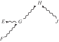
Figure 3: Free choice and causal order. An arbitrary causal order is depicted for random variables $E$, $F$, $G$, $H$ and $J$. The arrows correspond to the relation $\rightsquigarrow$. For example, $G$ lies in the future of $F$, i.e., $F\rightsquigarrow G$, but not of $J$, i.e., $J\not\rightsquigarrow G$. Because of the transitivity property, it follows that $F\rightsquigarrow E$, for example. In this setting we would say that, for instance, $G$ is free if it is uncorrelated with $F$ and $J$, i.e., $P_{GFJ}=P_{G}\times P_{FJ}$.

V Constraints on theories compatible with quantum theory

We discuss here the implication of some well-known results to our main question, whether an extension of quantum theory can have improved predictive power. Although they were not asking the same question, the works of Bell Bell and Leggett Leggett can be adapted to give constraints on such higher theories, and hence give special cases of the general theorem presented in Section VI, which excludes all alternative theories whose predictions are more informative than quantum theory.

V.1 Bipartite setup

The statements described below refer to a bipartite setup which involves two separate measurements, specified by parameters $A$ and $B$, and with outcomes $X$ and $Y$, respectively. As before, we consider a theory that allows us to compute predictions about these measurements, based on a parameter (or list of parameters) $Z$. Furthermore, in order to define free choices, we need to specify a causal order. The technical claims described in this section can be applied to any causal order that satisfies the following conditions:

• $A\rightsquigarrow X$ and $B\rightsquigarrow Y$;

• $A\not\rightsquigarrow Z$ and $B\not\rightsquigarrow Z$;

• $A\not\rightsquigarrow Y$ and $B\not\rightsquigarrow X$.

Condition (i) corresponds to the requirement that the measurement is specified before its outcome is obtained. Condition (ii) captures the fact that the parameters of the theory, $Z$, on which the predictions are based, should not only become available after the measurement process is started. This assumption can be considered necessary in order to reasonably talk about “predictions”. Finally, Condition (iii) demands that the arrangement of the two measurements should be such that neither of them lies in the future of the other. (Note that, assuming a relativistic space time structure, this would correspond to a setup where the measurements are space-like separated.) Together, the three conditions imply a causal order in which $A$ is considered free if $P_{ABYZ}=P_{A}\times P_{BYZ}$, and likewise for $B$. The causal orders respecting (i)–(iii) are illustrated in Figure 4.

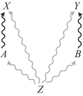
Figure 4: The causal orders for which our argument applies. We consider a setup with two separate measurements, one depending on a choice $A$ with outcome $X$, and the other with choice $B$ and outcome $Y$. Moreover, $Z$ denotes all extra parameters that may be used to make predictions about the outcomes. The figure illustrates all of the causal orders compatible with our requirements (i)–(iii). The black arrows originating from $A$ and $B$ are required, while each of the grey arrows originating from $Z$ is optional.

V.2 Local deterministic theories

Local deterministic theories were introduced in the work of Bell Bell , and, within the bipartite setup described above, are ones for which all conditional probabilities $P_{X|az}(x)$ and $P_{Y|bz}(y)$ are equal to either $0$ or $1$.

It follows using essentially the same argument used to prove Bell’s theorem that no locally deterministic theory can reproduce the predictions of quantum theory. To show this, it is sufficient to consider the correlations $P^{N}_{XY|AB\psi_{2}}$ that quantum theory predicts for the measurements on the maximally entangled state $\left|\psi_{2}\right\rangle$ defined in Section II.3. We state this as the following theorem.

Theorem 1 (No higher theories are locally deterministic).

Let $A$, $B$, $X$, $Y$ and $Z$ be RVs. Then at least one of the following cannot hold:

• Freedom of choice: $A$ and $B$ are free with respect to any of the causal orders depicted in Figure 4;

• Compatibility with quantum theory: $P_{XY|ABZ}$ is compatible with the predictions $P^{N}_{XY|AB\psi_{2}}$ of quantum theory (for some $N\geq 2$);

• Local determinism:

  $$P_{X|az}(x) \in\{0,1\}\quad\text{$\forall\ a,z$ s.t.\ $P_{AZ}(a,z)>0$}$$

  $$P_{Y|bz}(y) \in\{0,1\}\quad\text{$\forall\ b,z$ s.t.\ $P_{BZ}(b,z)>0$ .}$$

To prove this theorem, we use the correlation measure $I_{N}$ defined in Section II.3. The central idea is to show that, under the free choice assumption, all correlations explained by a locally deterministic model satisfy the inequality $I_{2}\geq 1$, which corresponds to the CHSH inequality CHSH . (The free choice assumption ensures that $P_{AB|z}$ has full support for each $z$, and hence that the conditional distributions $P_{X|az}$ and $P_{Y|bz}$ are well defined for any $a$, $b$, and $z$.) The assertion then follows from the fact that $I_{N}(P^{N}_{XY|AB\psi_{2}})=2-\sqrt{2}<1$ for $N=2$ (see Eq. 1).

V.3 Stochastic local causal theories

In his later work, Bell dropped the assumption of determinism and considered more general stochastic models. He adopted the following definition of locality called local causality, which leads to the relation $P_{XY|ABZ}=P_{X|AZ}P_{Y|BZ}$ Bell_nouvelle . Expanding the left hand side using Bayes’ rule, this can be broken down into four separate relations, $P_{X|ABZ}=P_{X|AZ}$, $P_{Y|ABZ}=P_{Y|BZ}$, $P_{X|ABYZ}=P_{X|ABZ}$ and $P_{Y|ABXZ}=P_{Y|ABZ}$. The first two of these have sometimes been termed parameter independence and imply that, even given access to $Z$, there cannot be signalling between the two measurement processes.

The last two conditions have been termed outcome independence. They do not have an obvious operational significance (such as no-signalling), and do not in general hold for the theories we consider in this work. We note, however, that they are automatically satisfied in any deterministic model, where each of the outcomes $X$ and $Y$ is a function of $A$, $B$, and $Z$. Conversely, as we argue below, if a theory is locally causal then the predictions it makes about the outcomes of measurements on the entangled state $\left|\psi_{2}\right\rangle=\frac{1}{\sqrt{2}}(\left|\uparrow\uparrow\right\rangle+\left|\downarrow\downarrow\right\rangle)$ are necessarily deterministic. (This is the essence of the EPR argument EPR .)

To see this, note that for any projective measurement (specified by $A=a$) applied to the first part of $\left|\psi_{2}\right\rangle$, there exists another projective measurement (specified by $B=b_{a}$) on the second part such that the outcomes are perfectly correlated. For example, if $A=a$ corresponds to the POVM $\{\left|\uparrow\right\rangle\!\!\left\langle\uparrow\right|,\left|\downarrow\right\rangle\!\!\left\langle\downarrow\right|\}$, and if we choose $B=b_{a}$ such that it corresponds to the same POVM, then $P_{XY|ab_{a}}(0,0)=P_{XY|ab_{a}}(1,1)=\frac{1}{2}$. This means that $X$ is determined by $Y$, i.e., $P_{X|ab_{a}yz}(x)=\delta_{x,y}\in\{0,1\}$ for all $a$, $x$, $y$ and $z$. Applying now the conditions of local causality, we obtain $P_{X|abyz}(x)=P_{X|az}(x)\in\{0,1\}$, which corresponds to the assumption of local determinism. Hence, there is an analogue of Theorem 1 in which the local determinism condition is weakened to Bell’s local causality condition.

We remark that, as we shall see below (Lemma 1), the freedom of choice assumption implies parameter independence, but is not strong enough to imply local causality, since it doesn’t imply outcome independence.

V.4 Leggett-type theories

In Leggett , Leggett introduced what he calls a “non-local hidden variable” model, which attempts to give an explanation of quantum correlations that is partly local and partly non-local. The presence of non-local hidden variables in his model leads to an incompatibility with the free choice assumption, and hence Leggett’s model is not a higher theory in the sense of the present work. However, since the behaviour of the non-local variables is not specified in Leggett’s model, we can consider a slightly modified version in which they are ignored (henceforth, when we speak about Leggett’s model, we refer to the local part of it). The model is then compatible with our notion of free choice, and offers improved predictive power for measurements on maximally entangled particles. We note that the model is not a full-fledged theory, as it only specifies how the outcomes of spin measurements are obtained.

Leggett’s model is based on the idea of assigning to each spin particle a three-dimensional vector (in addition to its quantum mechanical state). In particular, if we consider two spin particles, each measured on one side within the bipartite setup described above, we need to specify two such vectors, denoted ${\bf u}$ and ${\bf v}$, respectively. To connect this to our general discussion, we may think of these vectors as part of $Z$, i.e., $Z$ takes as values pairs $({\bf u},{\bf v})$. As above, we denote the choice of measurement on each side by $A$ and $B$. Restricting to projective spin measurements, the two choices may be labelled by three-dimensional vectors, denoted ${\bf a}$ and ${\bf b}$, respectively, indicating their orientation in space (see, for example, BBGKLLS for more details). The predictions for the measurement outcomes $X$ and $Y$, as prescribed by Leggett’s model, are then given by

$$P_{X|{\bf auv}}(x) = \frac{1}{2}(1+(-1)^{x}{\bf a}\cdot{\bf u})$$ (3)

$$P_{Y|{\bf buv}}(y) = \frac{1}{2}(1+(-1)^{y}{\bf b}\cdot{\bf v})\,.$$ (4)

In order to completely define the model, one would also need to assign probabilities to all possible values $Z=({\bf u},{\bf v})$, i.e., specify a probability distribution $P_{Z}$ (which, in general, depends on the quantum state). However, the following theorem, which is a corollary of results in Leggett ; GPKBZAZ ; BBGKLLS ; ColbeckRenner , implies that there is no such assignment for which Leggett’s model can be made compatible with quantum theory.

Theorem 2 (No higher theories obey the Leggett conditions).

Let $A$, $B$, $X$, $Y$ and $Z$ be RVs. Then there exists a quantum distribution, $P_{XY|AB\psi_{2}}$, such that at least one of the following cannot hold:

• Freedom of choice: $A$ and $B$ are free with respect to any of the causal orders depicted in Figure 4;

• Compatibility with quantum theory: $P_{XY|ABZ}$ is compatible with $P_{XY|AB\psi_{2}}$;

• Leggett rule: $P_{XY|ABZ}$ satisfies Eqs. 3 and 4 for all values $A=a$, $B=b$, and $Z=({\bf u},{\bf v})$.

We will not give a proof of this theorem here, since it follows from the more general results presented in the next section. To see this, it is sufficient to observe that, when measuring the entangled state $\left|\psi_{2}\right\rangle=\frac{1}{\sqrt{2}}(\left|\uparrow\uparrow\right\rangle+\left|\downarrow\downarrow\right\rangle)$, for instance, quantum theory prescribes that $P_{X|{\bf a}}(x)=\frac{1}{2}$, independently of the orientation ${\bf a}$ of the measurement. Conversely, Leggett’s model predicts a non-uniform distribution whenever the measurement orientation ${\bf a}$ is not orthogonal to the vector ${\bf u}$. The Leggett model is therefore more informative than quantum theory, and hence excluded by Lemma 3 (as well as the more general Theorem 3) below.

V.5 Other Constraints

Here we summarize a few other known constraints on theories compatible with quantum mechanics. One of the first results in this direction was that the quantum outcomes cannot be predetermined within a non-contextual model KS ; Bell_KS . In such a model, one assumes the existence of a map from the set of projectors to the set $\{0,1\}$ such that for every set of projectors that constitute a POVM, only one member of that set is mapped to $1$ (the element that maps to $1$ is interpreted as the outcome that will occur if a measurement described by that POVM is carried out). Such a model is non-contextual in that whether or not a particular outcome occurs depends only on the individual projectors, and not on the set of projectors making up the POVM. The Bell-Kochen-Specker theorem KS ; Bell_KS implies that no such assignment can exist if the Hilbert space dimension is at least $3$.

Hardy Hardy_ontbag later showed that within any extended theory, an infinite number of underlying states are required, even to describe a single qubit, and Montina Montina3 ; Montina proved, under the assumption of Markovian dynamics, that the number of real parameters that an extended theory needs to characterize a state in Hilbert space dimension $N$ is at least $2N-2$ (the same as the number of parameters needed to specify a pure quantum state up to global phase).

In addition, a claim in the same spirit as our non-extendibility theorem (presented in the next Section) has been obtained recently ChenMontina under the assumption of measurement non-contextuality, introduced in Spekkens_context .

VI The non-extendibility theorem

This section is devoted to the key result of this

Chapter ,

asserting that quantum theory is maximally informative. Stated informally, we make the following claim, first made in CR_ext .

Claim 1.

No alternative theory that is compatible with quantum theory and allows for free choice (with respect to the discussed causal orders) can give improved predictions.

The main technical statement is a generalization of the theorems discussed in the previous section. The setup is broadly the same, but instead of the condition that the higher theory remains compatible with quantum theory for measurements on maximally entangled states, we require this for a wider class of states. Furthermore, rather than considering theories that satisfy local determinism or the Leggett rule, the claim is about arbitrary theories that make improved predictions.

The main technical theorem is as follows (this should be read as a purely mathematical statement about bipartite pure states, whose significance to the extendibility of quantum theory will be explained subsequently).

Theorem 3.

Let $\left|\phi\right\rangle_{SD}$ be a pure state and let $\{\left|\hat{y}\right\rangle_{D}\}$ be a Schmidt basis on $D$. Then there exists a state $\left|\Gamma\right\rangle_{\tilde{S}\tilde{D}}$ and local POVMs $\{E_{x}^{a}\}$ and $\{F_{y}^{b}\}$ on $S\tilde{S}$ and $D\tilde{D}$, respectively, with $F_{y}^{b_{0}}=\left|\hat{y}\right\rangle\!\!\left\langle\hat{y}\right|_{D}\otimes\openone_{\tilde{D}}$ for some $b=b_{0}$, such that, for any RVs $A$, $B$, $X$, $Y$ and $Z$, at least one of the following cannot hold:

• Freedom of choice: $A$ and $B$ are free with respect to any of the causal orders depicted in Figure 4;

• Compatibility with quantum theory: $P_{XY|ABZ}$ is compatible with the prediction $P_{XY|AB(\phi\otimes\Gamma)}$ of quantum theory for the measurements $\{E_{x}^{a}\}$ and $\{F_{y}^{b}\}$ on $\left|\phi\right\rangle_{SD}\otimes\left|\Gamma\right\rangle_{\tilde{S}\tilde{D}}$.

• Improved predictions: $P_{Y|b_{0}\phi}$ is not as informative as $P_{Y|b_{0}Z}$.

To understand the implications of this theorem, consider a fixed measurement $\hat{a}$ on a system $S$. Assume that, according to quantum theory, the system (before the measurement) is in a pure state, denoted $\psi$, and that the measurement corresponds to a projective POVM, $\{\hat{E}^{\hat{a}}_{\hat{x}}\}$. Quantum theory then gives a probabilistic prediction $P_{\hat{X}|\hat{a}\psi}$ for the measurement outcome $\hat{X}$, which depends on $\psi$ and $\{\hat{E}^{\hat{a}}_{\hat{x}}\}$ (see Eq. 2). Our aim is to compare this quantum-mechanical prediction with the prediction $P_{\hat{X}|\hat{a}Z}$ that may be obtained by an alternative theory, whose parameters we denote by $Z$.

In order to relate this to the theorem, let us assume that the freedom of choice condition holds, from which it follows that the alternative theory is no-signalling (i.e., it would be impossible to signal in the higher theory, even knowing the parameter $Z$). We then consider the joint state of the measured system, $S$, and the measurement device, $D$, after the measurement $\hat{a}$. Following the discussion in Section III, according to quantum theory, this state can be assumed to have the form

$$\left|\phi\right\rangle_{SD}=\sum_{\hat{x}}\sqrt{\hat{E}^{\hat{a}}_{\hat{x}}}\left|\psi\right\rangle_{S}\otimes\left|\hat{x}\right\rangle_{D}\,\ .$$ (5)

Note that the POVM $\{F_{y}^{b_{0}}\}$ defined by Theorem 3 corresponds to a measurement of $D$ in the basis $\{\left|\hat{x}\right\rangle_{D}\}$. The outcome, $Y$, of this measurement can therefore be seen as a copy of the outcome $\hat{X}$ of the original measurement, specified by $\{\hat{E}^{\hat{a}}_{\hat{x}}\}$. In particular, the prediction that any theory compatible with quantum theory makes about $Y$ must be identical to the prediction it makes about $\hat{X}$, i.e., we have

$$P_{\hat{X}|\hat{a}\psi} =P_{Y|b_{0}\phi}$$

$$P_{\hat{X}|\hat{a}Z} =P_{Y|b_{0}Z}\ .$$

(Note that because the free choice assumption implies that the alternative theory is no-signalling, the prediction the alternative theory makes about $Y$ does not depend on $\hat{a}$, for example.)

We now apply Theorem 3 to $\left|\phi\right\rangle_{SD}$. If we assume that the alternative theory, in addition to being compatible with quantum theory, satisfies the freedom of choice assumption, then the third condition of the theorem cannot hold, i.e., $P_{Y|b_{0}\phi}$ is as informative as $P_{Y|b_{0}Z}$. Using the above identities, this directly carries over to the original measurement $\hat{a}$, i.e., the quantum-mechanical prediction $P_{\hat{X}|\hat{a}\psi}$ is as informative as the prediction $P_{\hat{X}|\hat{a}Z}$ of the alternative theory. We hence establish Claim 1.

VII Proof of Theorem 3

The theorem follows from three statements, which we formulate and prove separately. An overview of the argument is as follows. We consider the previously introduced bipartite scenario and any of the causal orders depicted in Figure 4. We begin by showing that free choice with respect to this causal order implies that the alternative theory is no-signalling (see Lemma 1). In the second part of the argument, we show that for measurements on maximally entangled states, if quantum theory is correct, no higher theory can give improved predictions about the outcomes (see Lemma 3). In the final part of the argument, we generalize this to measurements on an arbitrary bipartite entangled state. More precisely, we show that for any such state, there exist local measurements that generate correlations arbitrarily close to those generated by $r$ maximally entangled states for some sufficiently large integer $r$. Hence, from the second part of the argument, these measurements can have no improved predictions.

VII.1 Part I: No-signalling from free choice

In this part, we show that if $A$ and $B$ are free choices with respect to one of the given causal orders, then there is no signalling within the alternative theory (i.e. no signalling even given access to $Z$).

Lemma 1.

The freedom of choice assumption implies $P_{XZ|AB}=P_{XZ|A}$ and $P_{YZ|AB}=P_{YZ|B}$.

Proof.

That $A$ is free within the specified causal order implies $P_{A|BYZ}=P_{A}$ and hence

$$P_{YZA|B} =P_{YZ|B}\times P_{A|BYZ}=P_{A}\times P_{YZ|B}\,\text{, and}$$

$$P_{YZA|B} =P_{A|B}\times P_{YZ|AB}=P_{A}\times P_{YZ|AB}\,.$$

We therefore have $P_{YZ|AB}=P_{YZ|B}$. The relation $P_{XZ|AB}=P_{XZ|A}$ follows by symmetry. ∎

VII.2 Part II: Non-extendibility for measurements on maximally entangled states

In the second part of the argument, we show that the claim holds for particular measurements on maximally entangled pairs of qubits. The proof uses the correlation measure $I_{N}$ introduced in Section II.3. The following lemma shows that this measure, applied to a distribution $P_{XY|AB}$, gives a bound on how well any additional information, $Z$, can be correlated to the outcome $X$. Note that the lemma is independent of quantum theory and is simply a property of probability distributions.

Lemma 2.

Let $P_{XYZ|AB}$ be a distribution that obeys $P_{XZ|AB}=P_{XZ|A}$ and $P_{YZ|AB}=P_{YZ|B}$. Then, for all $a$ and $b$, we have

$$\bigl{\langle}D(P_{X|abz},P_{\bar{X}})\bigr{\rangle}_{z}\leq\frac{1}{2}I_{N}(P_{XY|AB})\,,$$ (6)

where $\langle\cdot\rangle_{z}$ denotes the average over the values of $Z$ (distributed according to $P_{Z|ab}$), and $P_{\bar{X}}$ denotes the uniform distribution on $X$.

The proof is based on an argument given in CR_ext , which develops results of BHK , BKP and ColbeckRenner .

Proof.

We first consider the quantity $I_{N}$ evaluated for the conditional distribution $P_{XY|ABz}=P_{XY|ABZ}(\cdot,\cdot|\cdot,\cdot,z)$, for any fixed $z$. The idea is to use this quantity to bound the variational distance between the conditional distribution $P_{X|az}$ and its negation, $1-P_{X|az}$, which corresponds to the distribution of $X$ if its values are interchanged. If this distance is small, it follows that the distribution $P_{X|az}$ is roughly uniform. Because this holds for any $Z=z$, $X$ must be independent of $Z$.

It is first worth noting that the conditions of the lemma ($P_{XZ|AB}=P_{XZ|A}$ and $P_{YZ|AB}=P_{YZ|B}$) imply $P_{X|ABZ}=P_{X|AZ}$ and $P_{Y|ABZ}=P_{Y|BZ}$ respectively, and together imply $P_{Z|AB}=P_{Z}$.

Let $P_{\bar{X}}$ be the uniform distribution on $X$. For $a_{0}:=0$, $b_{0}:=2N-1$, we have

$$I_{N}(P_{XY|ABz})$$

$$=P(X=Y|a_{0},b_{0},z)+\!\!\!\!\sum_{\genfrac{}{}{0.0pt}{}{a\in\mathcal{A}_{N},\,b\in\mathcal{B}_{N}}{|a-b|=1}}\!\!\!\!P(X\neq Y|a,b,z)$$

$$\geq D(1-P_{X|a_{0}b_{0}z},P_{Y|a_{0}b_{0}z})+\!\!\!\!\sum_{\genfrac{}{}{0.0pt}{}{a\in\mathcal{A}_{N},\,b\in\mathcal{B}_{N}}{|a-b|=1}}\!\!\!\!D(P_{X|abz},P_{Y|abz})$$

$$=D(1-P_{X|a_{0}z},P_{Y|b_{0}z})+\!\!\!\!\sum_{\genfrac{}{}{0.0pt}{}{a\in\mathcal{A}_{N},\,b\in\mathcal{B}_{N}}{|a-b|=1}}\!\!\!\!D(P_{X|az},P_{Y|bz})$$

$$\geq D(1-P_{X|a_{0}z},P_{X|a_{0}z})$$

$$=2D(P_{X|a_{0}b_{0}z},P_{\bar{X}})\,.$$ (7)

The first inequality follows from the fact that $D(P_{X|\Omega},P_{Y|\Omega})\leq P(X\neq Y|\Omega)$ for any event $\Omega$ (see Lemma 6 in Appendix A). Furthermore, we have used the conditions $P_{X|abz}=P_{X|az}$ and $P_{Y|abz}=P_{Y|bz}$, and the triangle inequality for $D$. By symmetry, this relation holds for all $a$ and $b$.

We now take the average over $z$ on both sides of (7). The left-hand-side gives

$$\sum_{z}P_{Z|ab}(z)I_{N}(P_{XY|ABz})$$

$$=\sum_{z}P_{Z}(z)I_{N}(P_{XY|ABz})$$

$$=\sum_{z}P_{Z|a_{0}b_{0}}(z)P(X=Y|a_{0},b_{0},z)+$$

$$\sum_{\genfrac{}{}{0.0pt}{}{a\in\mathcal{A}_{N},\,b\in\mathcal{B}_{N}}{|a-b|=1}}\sum_{z}P_{Z|ab}(z)P(X\neq Y|a,b,z)$$

$$=P(X=Y|a_{0},b_{0})+\!\!\!\!\sum_{\genfrac{}{}{0.0pt}{}{a\in\mathcal{A}_{N},\,b\in\mathcal{B}_{N}}{|a-b|=1}}\!\!\!\!P(X\neq Y|a,b,c)$$

$$=I_{N}(P_{XY|AB})\,,$$ (8)

where we used the condition $P_{Z|ab}=P_{Z}$ several times. Furthermore, taking the average on the right-hand-side of (7) yields

$$\sum_{z}P_{Z|ab}(z)D(P_{X|abz},P_{\bar{X}})=D(P_{XZ|ab},P_{\bar{X}}\times P_{Z|ab})\,,$$

which is equivalent to the left-hand side of (6). ∎

We now apply Lemma 2 to the quantum correlations $P^{N}_{XY|ab\psi_{2}}$ arising from measurements on the maximally entangled state $\psi_{2}$ (c.f. Section II.3). In the limit where $N$ tends to infinity, we have $\lim_{N\rightarrow\infty}I_{N}(P^{N}_{XY|AB})=0$, and hence we can establish that $P_{X|abz}=P^{N}_{X|ab\psi_{2}}$ for all $a$, $b$ and $z$ with $P^{N}_{ABZ|\psi_{2}}(a,b,z)>0$. Under the freedom of choice assumption and assuming compatibility with quantum theory (note that $P^{N}_{X|ab\psi_{2}}(x)=P_{\bar{X}}(x)=\frac{1}{2}$ for both $x=0$ and $x=1$) this implies $P_{X|az}=P^{N}_{X|a\psi_{2}}$ for all $a$ and $z$ with $P_{Z|a}(z)>0$. This means that $Z$ gives no additional information about the measurement outcome, $X$.

Taking Parts I and II together, we obtain the following lemma, which may be of independent interest.

Lemma 3 (No higher theories give improved predictions for pairs of maximally entangled qubits).

For any $\delta>0$ there exists an $N\in\mathbb{N}$ such that for any RVs $A$, $B$, $X$, $Y$ and $Z$, at least one of the following three conditions cannot hold:

• Freedom of choice: $A$ and $B$ are free with respect to any of the causal orders depicted in Figure 4;

• Compatibility with quantum theory: $P_{XY|ABZ}$ is compatible with $P_{XY|AB\psi_{2}}^{N}$;

• Improved predictions: There exists a value $A=a$ such that $\langle D(P_{X|az},P_{X|a\psi_{2}})\rangle_{z}>\delta$, where $\langle\cdot\rangle_{z}$ denotes the expectation value over $z$.

Hence, if an alternative theory is compatible with quantum theory and satisfies the freedom of choice assumption then the third condition cannot hold, i.e., $\langle D(P_{X|az},P_{X|a\psi_{2}})\rangle_{z}\leq\delta$. Since $\delta$ can be arbitrarily small, this implies that quantum theory is as informative as the alternative theory.

VII.3 Part III: Generalization to arbitrary measurements

The last part of the proof of Theorem 3 consists of generalizing Lemma 3, which applies to specific measurements on a maximally entangled state, to measurements on the general state $\left|\phi\right\rangle_{SD}$. The proof relies on the concept of embezzling states DamHay03 . These are entangled states that can be used to extract any desired maximally entangled state locally and without communication. More precisely, we will use the following lemma, which is implicit in DamHay03 .

Lemma 4.

For any $\delta>0$ and for any $k\in\mathbb{N}$ there exists a bipartite state $\left|\Gamma^{k}\right\rangle_{\tilde{S}\tilde{D}}$, the embezzling state, such that for any $m\leq k$, there exist local isometries, $U_{m}$ and $V_{m}$, on $\tilde{S}$ and $\tilde{D}$, respectively, that perform the transformation

$$U_{m}\otimes V_{m}:\,\left|\Gamma^{k}\right\rangle_{\tilde{S}\tilde{D}}\mapsto\left|\Gamma^{k}\right\rangle_{\tilde{S}\tilde{D}}\otimes\left|\psi_{m}\right\rangle_{S^{\prime}D^{\prime}}$$

with fidelity at least $1-\delta$, where $\left|\psi_{m}\right\rangle_{S^{\prime}D^{\prime}}:=\frac{1}{\sqrt{m}}\sum_{x=0}^{m-1}\left|\hat{x}\right\rangle_{S^{\prime}}\left|\hat{x}\right\rangle_{D^{\prime}}$ denotes a maximally entangled state of two $m$ dimensional systems.

Note that the state $\left|\phi\right\rangle_{SD}$ considered in Theorem 3 can be represented by its Schmidt decomposition as

$$\left|\phi\right\rangle_{SD}=\sum_{\hat{y}}\sqrt{p_{\hat{y}}}\left|\hat{y}\right\rangle_{S}\otimes\left|\hat{y}\right\rangle_{D}\ .$$

We now consider an embezzling state on $\tilde{S}\tilde{D}$ and use Lemma 4 to define isometries $\hat{U}$ and $\hat{V}$ on $S\tilde{S}$ and $D\tilde{D}$, respectively, which are controlled by the entry $\hat{y}$ in the registers $S$ or $D$, and build up entanglement between registers $S^{\prime}$ and $D^{\prime}$, i.e.,

$$\hat{U} =\sum_{\hat{y}}\left|\hat{y}\right\rangle\!\!\left\langle\hat{y}\right|_{S}\otimes U_{m(\hat{y})}$$

$$\hat{V} =\sum_{\hat{y}}\left|\hat{y}\right\rangle\!\!\left\langle\hat{y}\right|_{D}\otimes V_{m(\hat{y})}\ .$$

The integers $m(\hat{y})$ are chosen such that the state resulting from applying $\hat{U}\otimes\hat{V}$ to ${\left|\phi\right\rangle_{SD}\otimes\left|\Gamma^{k}\right\rangle_{\tilde{S}\tilde{D}}}$ is close to a state of the form

$$\Bigl{(}2^{-{r/2}}\sum_{\hat{y}}\sum_{\hat{y}^{\prime}=0}^{m(\hat{y})-1}\left|\hat{y},\hat{y}^{\prime}\right\rangle_{SS^{\prime}}\otimes\left|\hat{y},\hat{y}^{\prime}\right\rangle_{DD^{\prime}}\Bigr{)}\otimes\left|\Gamma^{k}\right\rangle_{\tilde{D}\tilde{S}}\,,$$

with $\sum_{\hat{y}}m(\hat{y})=2^{r}$, for some integer $r$. (This can be achieved to arbitrary precision for sufficiently large $k$ and $m(\hat{y})$.) Note that the first part of this state corresponds to $r$ maximally entangled pairs, $\left|\psi_{2}\right\rangle^{\otimes r}$, between the registers $SS^{\prime}$ and $DD^{\prime}$. We now construct the POVMs $\{E_{x}^{a}\}$ and $\{F_{y}^{b}\}$ by concatenating the operations $\hat{U}$ and $\hat{V}$ with the projective measurements along the vectors $\left|(\frac{a_{i}}{2N}+x_{i})\pi\right\rangle$ and $\left|(\frac{b_{i}}{2N}+y_{i})\pi\right\rangle$ introduced in Section II.3. More precisely, we define

$$E_{x}^{a} :=\hat{U}^{\dagger}\cdot\Bigl{[}\Bigl{(}\bigotimes_{i=1}^{r}\left|(\tfrac{a_{i}}{2N}+x_{i})\pi\right\rangle\!\!\left\langle(\tfrac{a_{i}}{2N}+x_{i})\pi\right|\Bigr{)}_{DD^{\prime}}\!\!\!\!\!\otimes\openone_{\tilde{D}}\Bigr{]}\cdot\hat{U}$$

$$F_{y}^{b} :=\hat{V}^{\dagger}\cdot\Bigl{[}\Bigl{(}\bigotimes_{i=1}^{r}\left|(\tfrac{b_{i}}{2N}+y_{i})\pi\right\rangle\!\!\left\langle(\tfrac{b_{i}}{2N}+y_{i})\pi\right|\Bigr{)}_{SS^{\prime}}\!\!\!\!\!\otimes\openone_{\tilde{S}}\Bigr{]}\cdot\hat{V}$$

with $a=(a_{1},\ldots,a_{r})\in\mathcal{A}_{N}^{\times r}$ and $b=(b_{1},\ldots,b_{r})\in\mathcal{B}_{N}^{\times r}$, for some large $N$. In addition we define

$$F_{y}^{b_{0}}=\left|\hat{y}\right\rangle\!\!\left\langle\hat{y}\right|_{S}\otimes\openone_{\tilde{S}}\ .$$

Assume now that the freedom of choice as well as the compatibility with quantum theory assumption are satisfied. Furthermore, let $X=(\hat{X},\hat{X}^{\prime})$ and $Y=\hat{Y}$ be the outcomes of the measurements $A=a_{0}:=(0,\ldots,0)$ and $B=b_{0}$, respectively. By choosing the orientation of the vectors $\left|\uparrow\right\rangle$ and $\left|\downarrow\right\rangle$ of Section II.3 appropriately, we can arrange it so that quantum theory predicts that the outcomes of the measurements of $a_{0}$ and $b_{0}$ are in agreement, in the sense that $\hat{X}=Y$ holds with probability $1$. Hence, together with the no-signalling conditions (c.f. Lemma 1) we find that

$$P_{Y|b_{0}(\psi\otimes\Gamma)} =P_{\hat{X}|a_{0}(\psi\otimes\Gamma)}$$

$$P_{Y|b_{0}Z} =P_{\hat{X}|a_{0}Z}$$

Lemma 3 implies that, $P_{X|a_{0}(\psi\otimes\Gamma)}$ must be as informative as $P_{X|a_{0}Z}$. In particular, the same relation holds for the marginals of these distributions, i.e, $P_{\hat{X}|a_{0}(\psi\otimes\Gamma)}$ is as informative as $P_{\hat{X}|a_{0}Z}$. Combining this with the above identities we find that $P_{Y|b_{0}\psi}=P_{Y|b_{0}(\psi\otimes\Gamma)}$ is as informative as $P_{Y|b_{0}Z}$, thus concluding the proof of Theorem 3.

VIII Alternative theories are equivalent to quantum theory

In this section, we discuss an implication of the non-extendibility theorem (Theorem 3) to a long-standing debate on the nature of the quantum mechanical wave function. The debate centres around whether it should be interpreted as a subjective quantity, for example a state of knowledge about some underlying physical reality, or whether it should instead be interpreted as objective (real). The wave function could be considered subjective if there existed an alternative theory, with predictions based on a parameter $Z$, that is at least as informative as quantum theory, and in which two different wave functions, say $\psi$ and $\psi^{\prime}$, are compatible with the same value of the parameter, say $Z=z$. Formally, this would mean that there exist $z$, $\psi$, and $\psi^{\prime}\neq\psi$ such that $P_{Z\Psi}(z,\psi)>0$ and $P_{Z\Psi}(z,\psi^{\prime})>0$. This is sometimes called a $\psi$-epistemic view of the wave function and contrasts with the $\psi$-ontic, or objective, view HarSpek (we refer to CFS ; Spekkens ; LeiSpek for arguments in favour of the $\psi$-epistemic view). In the latter, the wave function is uniquely determined by the parameters of any alternative theory that is at least as informative as quantum theory, i.e., there exists a (deterministic) function, $f$ such that $\Psi=f(Z)$.

Our result is based on the following simple lemma, which asserts that, if an alternative theory is equally informative as quantum theory then the wave function is indeed uniquely determined by the parameter of the alternative theory.

Lemma 5.

Suppose $\{E^{a}_{x}\}$ form a tomographically complete set of POVMs, and $A$, $X$, $\Psi$ and $Z$ are RVs such that:

• $A$ is a free choice with respect to a causal order in which $A\not\rightsquigarrow Z$ and $A\not\rightsquigarrow\Psi$.

• $P_{X|AZ}$ is at least as informative as $P_{X|A\Psi}$, where $P_{X|a\psi}(x)=\mathrm{tr}(E^{a}_{x}\psi)$.

• $P_{X|A\Psi}$ is at least as informative as $P_{X|AZ}$.

Then there exists a function, $f$, such that $\Psi=f(Z)$.

Proof.

If $P_{X|AZ}$ is at least as informative as $P_{X|A\Psi}$, then there exists a distribution $\bar{P}_{XZ\Psi|A}$ such that

$$P_{X|a\psi} =\sum_{z}\bar{P}_{XZ|a\psi}(\cdot,z)\ \ \text{$\forall\ a,\psi$}$$

$$P_{X|az} =\sum_{\psi}\bar{P}_{X\Psi|az}(\cdot,\psi)\ \ \text{$\forall\ a,z$}.$$

(we drop the bar on $P$ in the following, and simply use $P_{XZ\Psi|A}$ to denote this distribution). We have

$$P_{X|az\psi}=P_{X|az}$$

for all $a,z,\psi$ that have a non-zero joint probability, i.e., $P_{AZ\Psi}(a,z,\psi)>0$. Likewise, if $P_{X|A\Psi}$ is at least as informative as $P_{X|AZ}$ then

$$P_{X|az\psi}=P_{X|a\psi}$$

holds under the same condition. Combining these expressions gives

$$P_{X|a\psi}=P_{X|az}\,.$$ (9)

If $A$ is a free choice, we have $P_{AZ\Psi}=P_{A}\times P_{Z\Psi}$, hence (9) holds provided that $P_{Z\Psi}(z,\psi)>0$ and $P_{A}(a)>0$.

Let now $z$, $\psi$ and $\psi^{\prime}$ be such that $P_{Z\Psi}(z,\psi)>0$ and $P_{Z\Psi}(z,\psi^{\prime})>0$. From (9), this implies $P_{X|a\psi}=P_{X|a\psi^{\prime}}$ for all $a$ such that $P_{A}(a)>0$. Since the set of measurements with $P_{A}(a)>0$ is tomographically complete, this can only be satisfied if $\psi=\psi^{\prime}$. It hence follows that there exists a function $f$ such that $\Psi=f(Z)$. ∎

Combining Theorem 3 with Lemma 5, we can establish the main result of this section, which we state informally as follows.

Claim 2.

CR_wavefn In any alternative theory that is at least as informative as quantum theory and compatible with free choice (with respect to the discussed causal orders), there is a one-to-one correspondence between the parameters of the alternative theory and the quantum state (up to a possible removable degeneracy in the parameters of the alternative theory).

To establish this, as before, we use $Z$ to denote the parameters of the higher theory. Theorem 3 shows that under the freedom of choice assumption, quantum theory is at least as informative as any alternative theory. We hence satisfy the conditions of Lemma 5 so find $\Psi=f(Z)$, for some function $f$. Furthermore, since $Z$ cannot improve the predictions for any $\Psi=\psi$, any $z$ in $f^{-1}(\psi)$ must give identical predictions. Hence, if $f^{-1}(\psi)$ contains more than one element, this corresponds to a removable degeneracy in the parameters of the alternative theory.

Related work

An interpretation of the wave function as a subjective state of knowledge about some underlying theory has also been ruled out by Pusey et al. PBR via a different argument using different assumptions which we now summarize. They consider the preparation of multiple quantum systems, with states $\Psi_{i}$, where each system is associated with a particular parameter in the higher theory, $Z_{i}$. Pusey et al. assume that the joint distribution of these is product, i.e.

$$P_{Z_{1}Z_{2}\ldots\Psi_{1}\Psi_{2}\ldots}=P_{Z_{1}\Psi_{1}}\times P_{Z_{2}\Psi_{2}}\times\ldots\,.$$ (10)

Starting from this assumption, they show that there cannot exist two distinct states, $\psi$ and $\psi^{\prime}$, such that for each $i$ there exists a value of $Z_{i}=z_{i}$ satisfying $P_{Z_{i}\Psi_{i}}(z_{i},\psi)>0$ and $P_{Z_{i}\Psi_{i}}(z_{i},\psi^{\prime})>0$.

We note that the product nature of the joint distribution, Eq. (10), is related to free choice of preparation. In particular, it implies

$$P_{\Psi_{1}Z_{2}\ldots Z_{N}\Psi_{2}\ldots\Psi_{N}}=P_{\Psi_{1}}\times P_{Z_{2}\ldots Z_{N}\Psi_{2}\ldots\Psi_{N}}\,.$$

If we take the causal order to be such that $\Psi_{i}\not\rightsquigarrow\Psi_{j}$ and $\Psi_{i}\not\rightsquigarrow Z_{j}$ for $j\neq i$ (as would be natural if we make space-like separated preparations), then this is equivalent to saying that $\Psi_{1}$ can be chosen freely.

It was subsequently noted Hall_PBR that the separability assumption can be weakened, in essence to the assumption that there exists a particular set of parameters in the higher theory that are compatible with every product state composed of $\psi$ and $\psi^{\prime}$, i.e., there exist values of the parameters, $z_{1},\ldots,z_{N}$, such that

$$P_{Z_{1}\ldots Z_{N}\Psi_{1}\ldots\Psi_{N}}(z_{1},\ldots,z_{N},\psi^{(}\phantom{}{}^{\prime}\phantom{}{}^{)},\ldots,\psi^{(}\phantom{}{}^{\prime}\phantom{}{}^{)})>0\,,$$

where each $\psi^{(}\phantom{}{}^{\prime}\phantom{}{}^{)}$ is independently either $\psi$ or $\psi^{\prime}$ (so that the above represents $2^{N}$ conditions). This condition can be further weakened SF such that the parameters of the alternative theory for multiple systems need not be made up only of the individual parts, but could be replaced or supplemented with global parameters (provided these are also compatible with all the product state preparations).

An alternative argument against an interpretation of the quantum state as a state of knowledge about an underlying reality can be found in Hardy_PBR .

We remark that some models in which the wave function is subjective have been developed for restricted scenarios. For example, by modifying an earlier model by Bell Bell_ch1 , Lewis et al. constructed a model for a single qubit in which the wave function is subjective, and extended that model to arbitrary dimensions LJBR . These models are not in conflict with Claim 2 because they treat only single systems, and cannot be extended to bipartite scenarios while allowing for free choice with respect to one of the causal orders of Figure 4.

IX Discussion

The main statements described in this

Chapter

about the completeness of quantum theory are based on two assumptions. One of them is that quantum theory is correct, and is implicit in the question of completeness. The other is that of free choice within a natural causal order. It is worth commenting on the existence of alternative models that are not compatible with this assumption.

A prominent example is the de Broglie-Bohm model deBroglie ; Bohm which recreates quantum correlations, providing higher explanation in the form of hidden particle positions. These can be thought of as parameters of a higher theory that would allow perfect predictions of the outcomes. However, introducing these parameters comes at a price: it is incompatible with the freedom of choice assumption of our theorems. In fact, for the bipartite setting discussed above, if $Z$ includes the particle positions of the de Broglie-Bohm model, we have some non-local behaviour, so that $P_{X|abz}=P_{X|az}$, for instance, does not hold. Thus, given Lemma 1, it follows that $A$ and $B$ cannot be free choices with respect to any of the causal orders of Figure 4.

There are at least two ways to avoid our conclusions. The first is to maintain free choice, but assume that the alternative theory has a different causal order (in particular, one in which either $A\not\rightsquigarrow Y$ or $B\not\rightsquigarrow X$ does not hold). The second is to consider alternative theories without free choice, in which the measurement settings $A$ and $B$ may depend on the additional parameters $Z$ (sometimes, this view is argued for by imagining that the additional parameters are permanently hidden).

One may take the view that the freedom of choice assumption, which demands complete independence between the chosen settings and the other variables, is relatively strong, and perhaps contemplate alternative theories where this assumption is weakened. Some results in this direction can be found in CR_free , where a theorem similar to Lemma 3 is established under a relaxed free choice assumption, and provided there is no signalling at the level of the underlying theory.

Finally, we note that the result presented here has a generic application in quantum cryptography. Standard security proofs for schemes such as quantum key distribution BB84 ; Ekert are based on the assumption (usually not stated explicitly) that quantum theory is complete. If this were not the case, it could be that a scheme is proven secure within quantum theory, yet an adversary can break it by exploiting information available in a higher theory. However, the non-extendibility theorem, Theorem 3, implies that it is sufficient to make only the weaker assumption that quantum theory is correct, since this implies completeness.

Appendix A Variational Distance

The following is a list of the main properties of the variational distance $D(\cdot,\cdot)$ used in this work:

• $D(\cdot,\cdot)$ is a metric on the space of probability distributions.

• $D(\cdot,\cdot)$ is upper bounded by $1$.

• The variational distance of marginal distributions cannot be larger than that of the joint distributions: $D(P_{X},Q_{X})\leq D(P_{XY},Q_{XY})$ for any $P_{XY}$ and $Q_{XY}$.

• It is convex: If $\{\alpha_{i}\}$ satisfy $\alpha_{i}\geq 0$ and $\sum_{i}\alpha_{i}=1$, and $\{P^{i}_{X}\}$ and $\{Q^{i}_{X}\}$ are sets of distributions over $X$, then $D(\sum_{i}\alpha_{i}P^{i}_{X},\sum_{i}\alpha_{i}Q^{i}_{X})\leq\sum_{i}\alpha_{i}D(P^{i}_{X},Q^{i}_{X})$.

• For a joint distribution $P_{XY}$, the variational distribution of the marginal distributions is bounded by the probability that the RVs $X$ and $Y$ have different values: $D(P_{X},P_{Y})\leq P(X\neq Y)$.

The first four properties follow straightforwardly from the definition. The last is proved in the following.

Lemma 6.

Let $X$ and $Y$ be two random variables jointly distributed according to $P_{XY}$. Then the variational distance between the marginal distributions $P_{X}$ and $P_{Y}$ is bounded by

$$D(P_{X},P_{Y})\leq P(X\neq Y)\,.$$

Proof.

Let $P_{XY}^{\neq}:=P_{XY|X\neq Y}$ be the joint distribution of $X$ and $Y$ conditioned on the event that they are not equal. Similarly, define $P_{XY}^{=}:=P_{XY|X=Y}$. We then have

$$P_{XY}=p_{\neq}P_{XY}^{\neq}+(1-p_{\neq})P_{XY}^{=}$$

where $p_{\neq}:=P(X\neq Y)$. By linearity, the marginals of these distributions satisfy the same relation, i.e.,

$$P_{X} = p_{\neq}P_{X}^{\neq}+(1-p_{\neq})P_{X}^{=}$$

$$P_{Y} = p_{\neq}P_{Y}^{\neq}+(1-p_{\neq})P_{Y}^{=}\,.$$

Hence, by convexity of the variational distance,

$$D(P_{X},P_{Y}) \leq p_{\neq}D(P_{X}^{\neq},P_{Y}^{\neq})+(1-p_{\neq})D(P_{X}^{=},P_{Y}^{=})$$

$$\leq p_{\neq}\,,$$

where the last inequality follows because the variational distance is at most 1, and $D(P_{X}^{=},P_{Y}^{=})=0$. ∎