Principal Component Analysis with
Noisy and/or Missing Data

Abstract

We present a method for performing Principal Component Analysis (PCA) on noisy datasets with missing values. Estimates of the measurement error are used to weight the input data such that compared to classic PCA, the resulting eigenvectors are more sensitive to the true underlying signal variations rather than being pulled by heteroskedastic measurement noise. Missing data is simply the limiting case of weight=0. The underlying algorithm is a noise weighted Expectation Maximization (EM) PCA, which has additional benefits of implementation speed and flexibility for smoothing eigenvectors to reduce the noise contribution. We present applications of this method on simulated data and QSO spectra from the Sloan Digital Sky Survey.

1 Introduction

Principal Component Analysis (PCA) is a powerful and widely used technique to analyze data by forming a custom set of “principal component” eigenvectors that are optimized to describe the most data variance with the fewest number of components (Pearson, 1901; Hotelling, 1933; Jolliffe, 2002). With the full set of eigenvectors the data may be reproduced exactly, i.e., PCA is a transformation which can lend insight by identifying which variations in a complex dataset are most significant and how they are correlated. Alternately, since the eigenvectors are optimized and sorted by their ability to describe variance in the data, PCA may be used to simplify a complex dataset into a few eigenvectors plus coefficients, under the approximation that higher-order eigenvectors are predominantly describing fine tuned noise or otherwise less important features of the data. Example applications within astronomy include classifying spectra by fitting them to PCA templates (Pâris et al., 2011; Connolly & Szalay, 1999), describing Hubble Space Telescope point spread function variations (Jee et al., 2007), and reducing the dimensionality of Cosmic Microwave Background map data prior to analysis (Bond, 1995).

A limitation of classic PCA is that it does not distinguish between variance due to measurement noise vs. variance due to genuine underlying signal variations. Even when an estimate of the measurement variance is available, this information is not used when constructing the eigenvectors, e.g., by deweighting noisy data.

A second limitation of classic PCA is the case of missing data. In some applications, certain observations may be missing some variables and the standard formulas for constructing the eigenvectors do not apply. For example within astronomy, observed spectra do not cover the same rest-frame wavelengths of objects at different redshifts, and some wavelength bins may be masked due to bright sky lines or cosmic ray contamination. Missing data is an extreme case of noisy data, where missing data is equivalent to data with infinite measurement variance.

This work describes a PCA framework which incorporates estimates of measurement variance while solving for the principal components. This optimizes the eigenvectors to describe the true underlying signal variations without being unduly affected by known measurement noise. Code which implements this algorithm is available at https://github.com/sbailey/empca .

Jolliffe (2002) §13.6 and §14.2 review prior work on PCA with missing data and incorporating weights into PCA. Most prior work focuses on the identification and removal of outlier data, interpolation over missing data, or special cases such as when the weights can be factorized into independent per-observation and per-variable weights. Gabriel & Zamir (1979), Wentzell et al. (1997), Tipping & Bishop (1999), and Srebro & Jaakkola (2003) present iterative solutions for the case of general weights, though none of these find the true PCA solution with orthogonal eigenvectors optimally ranked by their ability to describe the data variance. Instead, they find an unsorted set of non-orthogonal vectors which as a set are optimized to describe the data variance, but individually they are not the optimal linear combinations to describe the most variance with the fewest vectors. Their methods are sufficient for weighted lower-rank matrix approximation, but they lack the potential data insight from optimally combining and sorting the eigenvectors to see which components contribute the most variation.

Within the astronomy literature, Connolly & Szalay (1999) discuss how to interpolate over missing data and use PCA eigenspectra to fit noisy and/or missing data, but they do not address the case of how to generate eigenspectra from noisy but non-missing data. Blanton & Roweis (2007) generate template spectra from noisy and missing data using Non-negative Matrix Factorization (NMF). This method is similar to PCA with the constraint that the template spectra are strictly positive, while not requiring the templates to be orthonormal. Tsalmantza & Hogg (2012) present a more general “Heteroskedastic Matrix Factorization” approach to study Sloan Digital Sky Survey spectra while properly accounting for measurement noise. Their underlying goal is similar to this work, though with an algorithmically different implementation.

The methods presented here directly solve for the PCA eigenvectors with an iterative solution based upon Expectation Maximization PCA (EMPCA). Roweis (1997) describes an unweighted version of EMPCA, including a method for interpolating missing data, but he does not address the issue of deweighting noisy data. We also take advantage of the iterative nature of the solution to bring unique extensions to PCA, such as noise-filtering the eigenvectors during the solution.

The approach taken here is fundamentally pragmatic. For example, if one is interested in generating eigenvectors to describe 99% of the signal variance, it likely doesn’t matter if an iterative algorithm has “only” converged at the level of $10^{-5}$ even if the machine precision is formally $10^{-15}$. We discuss some of the limitations of Weighted EMPCA in §8, but ultimately we find that these issues are not limiting factors for practical applications.

This work was originally developed for PCA analysis of astronomical spectra and examples are given in that context. It should be noted, however, that these methods are generally applicable to any PCA application with noisy and/or missing data — nothing in the underlying methodology is specific to astronomical spectra.

2 Notation

This paper uses the following notation: Vectors use arrows, $\vec{x}$, while $x_{i}$ represents the scalar element $i$ of vector $\vec{x}$. For sets of vectors, $\vec{x}_{j}$ represent vector number $j$ (not element $j$ of vector $\vec{x}$). Matrices are in boldface, $\mathbf{X}$. To denote vectors formed by selected columns or rows of a matrix, we use $\vec{\mathbf{X}}^{\mathrm{col}}_{j}$ for the vector formed from column $j$ of matrix $\mathbf{X}$ and $\vec{\mathbf{X}}^{\mathrm{row}}_{i}$ for the vector formed from row $i$ of matrix $\mathbf{X}$. The scalar element at row $i$ column $j$ of matrix $\mathbf{X}$ is $\mathbf{X}_{ij}$.

For reference, we summarize the names of the primary variables here: $\mathbf{X}$ is the data matrix with $n_{\rm var}$ rows of variables and $n_{\rm obs}$ columns of observations. $\mathbf{P}$ is the PCA eigenvector matrix with $n_{\rm var}$ rows of variables and $n_{\rm vec}$ columns of eigenvectors; $\vec{\phi}$ is a single eigenvector. These eigenvectors may fit the data using a matrix of coefficients $\mathbf{C}$, where $\mathbf{C}_{kj}$ is the contribution of eigenvector $k$ to observation $j$. Indices $i$, $j$, and $k$ index variables, observations, and eigenvectors respectively. $\vec{\mathbf{X}}$ is the vector formed by stacking the columns of matrix $\mathbf{X}$. The measurement covariance of dataset $\vec{\mathbf{X}}$ is $\mathbf{V}$, while $\mathbf{W}$ is the weights matrix for dataset $\mathbf{X}$ for the case of independent measurement noise such that $\mathbf{W}$ has the same dimensions as $\mathbf{X}$.

3 Classic PCA

For an accessible tutorial on classic PCA, see Schlens (2009). A much more complete treatment is found in Jolliffe (2002). Algorithmically, the steps are simple: The principal components $\{\vec{\phi}_{k}\}$ of a dataset are simply the eigenvectors of the covariance of that dataset, sorted by their descending eigenvalues. A new observation $\vec{y}$ may be approximated as

$$\vec{y}=\vec{\mu}+\sum_{k}c_{k}\vec{\phi}_{k}$$ (1)

where $\vec{\mu}$ is the mean of the initial dataset and $c_{i}$ is the reconstruction coefficient for eigenvector $\vec{\phi}_{i}$. For the rest of this paper, we will assume that $\vec{\mu}$ has already been subtracted from the data, i.e., $\vec{y}\leftarrow(\vec{y}-\vec{\mu})$.

To find a particular coefficient $c_{k^{\prime}}$, take the dot product of both sides with $\vec{\phi}_{k^{\prime}}$, noting that because of the eigenvector orthogonality, $\vec{\phi}_{k}\cdot\vec{\phi}_{k^{\prime}}=\delta_{kk^{\prime}}$ (Kroeneker-delta):

$$\vec{y}\cdot\vec{\phi}_{k^{\prime}} = \sum_{k}c_{k}\vec{\phi}_{k}\cdot\vec{\phi}_{k^{\prime}}$$ (2)

$$= \sum_{k}c_{k}\delta_{kk^{\prime}}$$ (3)

$$= c_{k^{\prime}}$$ (4)

Note that the neither the solution of $\{\vec{\phi}_{k}\}$ nor $\{c_{k}\}$ makes use of any noise estimates or weights for the data. As such, classic PCA solves the minimization problem

$$\chi^{2}=\sum_{i,j}[\mathbf{X}-\mathbf{P}\mathbf{C}]_{ij}^{2}$$ (5)

where $\mathbf{X}$ is a dataset matrix whose columns are observations and rows are variables, $\mathbf{P}$ is a matrix whose columns are the principal components $\{\vec{\phi}_{k}\}$ to find, and $\mathbf{C}$ is a matrix of coefficients to fit $\mathbf{X}$ using $\mathbf{P}$. For clarity, the dimensions of these matrices are: $\mathbf{X}[n_{\mathrm{var}},n_{\mathrm{obs}}]$, $\mathbf{P}[n_{\mathrm{var}},n_{\mathrm{vec}}]$, and $\mathbf{C}[n_{\mathrm{vec}},n_{\mathrm{obs}}]$, where $n_{\mathrm{obs}}$, $n_{\mathrm{var}}$, and $n_{\mathrm{vec}}$ are the number of observations, variables, and eigenvectors respectively. For example, when performing PCA on spectra, $n_{\mathrm{obs}}$ is the number of spectra, $n_{\mathrm{var}}$ is the number of wavelength bins per spectrum, and $n_{\mathrm{vec}}$ is the number of eigenvectors used to describe the data, which may be smaller than the total number of possible eigenvectors.

4 Adding Weights to PCA

The goal of this work is to solve for the eigenvectors $\mathbf{P}$ while incorporating a weights matrix $\mathbf{W}$ on the dataset $\mathbf{X}$:

$$\chi^{2}=\sum_{i,j}\mathbf{W}_{ij}[\mathbf{X}-\mathbf{P}\mathbf{C}]_{ij}^{2}$$ (6)

We also describe the more general cases of per-observation covariances $\mathbf{V}_{j}$:

$$\chi^{2}=\sum_{\mathrm{obs}~{}j}\left(\vec{\mathbf{X}}^{\mathrm{col}}_{j}-\mathbf{P}\vec{\mathbf{C}}^{\mathrm{col}}_{j}\right)^{T}\mathbf{V}_{j}^{-1}\left(\vec{\mathbf{X}}^{\mathrm{col}}_{j}-\mathbf{P}\vec{\mathbf{C}}^{\mathrm{col}}_{j}\right)$$ (7)

where we have used the notation that $\vec{\mathbf{X}}^{\mathrm{col}}_{j}$ is the vector formed from the $j$th column of the matrix $\mathbf{X}$, and similarly for $\vec{\mathbf{C}}^{\mathrm{col}}_{j}$. In the most general case, there is covariance $\mathbf{V}$ between all variables of all observations, i.e., we seek to minimize

$$\chi^{2}=\left(\vec{\mathbf{X}}-[\mathbf{P}]\vec{\mathbf{C}}\right)^{T}\mathbf{V}^{-1}\left(\vec{\mathbf{X}}-[\mathbf{P}]\vec{\mathbf{C}}\right)$$ (8)

Where $\vec{\mathbf{X}}$ and $\vec{\mathbf{C}}$ are the vectors formed by concatenating all columns of $\mathbf{X}$ and $\mathbf{C}$, and $[\mathbf{P}]$ is the matrix formed by stacking $\mathbf{P}$ $n_{\rm obs}$ times.

This allows one to incorporate error estimates on heteroskedastic data such that particularly noisy data does not unduly influence the solution. We will solve this problem using an iterative method known within the statistics community as “Expectation Maximization”.

5 Weighted Expectation Maximization PCA

5.1 Expectation Maximization PCA

Expectation Maximization (EM) is an iterative technique for solving parameters to maximize a likelihood function for models with unknown hidden (or latent) variables (Dempster, Laird, & Rubin, 1977). Each iteration involves two steps: finding the expectation value of the hidden variables given the current model (E-step), and then modifying the model parameters to maximize the fit likelihood given the estimates of the hidden variables (M-step).

As applied to PCA, the parameters to solve are the eigenvectors, the latent variables are the coefficients $\{c\}$ for fitting the data using those eigenvectors, and the likelihood is the ability of the eigenvectors to describe the data. To solve the single most significant eigenvector, start with a random vector $\vec{\phi}$ of length $n_{\rm var}$. For each observation $\vec{x}_{j}$, solve the coefficient $c_{j}=\vec{x}_{j}\cdot\vec{\phi}$ which best fits that observation using $\vec{\phi}$. Then using those coefficients, update $\vec{\phi}$ to find the vector that best fits the data given those coefficients: $\vec{\phi}\leftarrow\sum_{j}c_{j}\vec{x}_{j}/\sum_{j}c_{j}^{2}$. Then normalize $\vec{\phi}$ to unit length and iterate the solutions to $\{c\}$ and $\vec{\phi}$ until converged. In summary:

	$\vec{\phi}\leftarrow$ random vector of length $n_{\rm var}$
repeat until converged:
	For each observation $\vec{x}_{j}$:
		$c_{j}\leftarrow\vec{x}_{j}\cdot\vec{\phi}$	E-step
	$\vec{\phi}\leftarrow\sum_{j}c_{j}\vec{x}_{j}/\sum_{j}c_{j}^{2}$		M-step
	$\vec{\phi}\leftarrow\vec{\phi}/|\vec{\phi}|$		Renormalize
return $\vec{\phi}$

This generates a vector $\vec{\phi}$ which is the dominant PCA eigenvector of the dataset $\mathbf{X}$, where the observations $\vec{x}_{j}$ are the columns of $\mathbf{X}$. The expectation step finds the coefficients $\{c_{j}\}$ which best fit $\mathbf{X}$ using $\vec{\phi}$ (see equations 2 to 4). The likelihood maximization step then uses those coefficients to update $\vec{\phi}$ to minimize

$$\chi^{2}=\sum_{\mathrm{var}~{}i,~{}\mathrm{obs}~{}j}({\bf X}_{ij}-c_{j}\phi_{i})^{2}$$ (9)

In practice the normalization $\sum_{j}c_{j}^{2}$ in the M-step is unnecessary since $\vec{\phi}$ is renormalized to unit length after every iteration.

At first glance, it can be surprising that this algorithm works at all. Its primary enabling feature is that at each iteration the coefficients $\{c_{j}\}$ and vector $\vec{\phi}$ minimize the $\chi^{2}$ better than the previous iteration. The $\chi^{2}$ of equation 9 has a single minimum (Srebro & Jaakkola, 2003), thus when any minimum is found it is the true global minimum. It is possible, however, to also have saddle points to which the EMPCA algorithm could converge from particular starting points. It is easy to test solutions for being at a saddle point and restart the iterations as needed.

The specific convergence criteria are application specific. One pragmatic option is that the eigenvector itself is changing slowly, i.e., $|\Delta\vec{\phi}|<\epsilon$. Alternately, one could require that the change in likelihood (or $\Delta\chi^{2}$) from one iteration to the next is below some threshold. Convergence and uniqueness will be discussed in $\S$8.1 and §8.2. For now we simply note that many PCA applications are interested in describing 95% or 99% of the data variance, and the above algorithm typically converges very quickly for this level of precision, even for cases when the formal computational machine convergence may require many iterations.

To find additional eigenvectors, subtract the projection of $\vec{\phi}$ from ${\bf X}$ and repeat the algorithm. Continue this procedure until enough eigenvectors have been solved that the remaining variance is consistent with the expected noise of the data, or until enough eigenvectors exist to approximate the data with the desired fidelity. If only a few eigenvectors are needed for a large dataset, this algorithm can be much faster than classic PCA which requires solving for all eigenvectors whether or not they are needed. Scaling performance will be discussed further in $\S$8.4.

5.2 EMPCA with per-observation weights

The above algorithm treats all data equally when solving for the eigenvectors and thus is equivalent to classic PCA. If all data are of approximately equal quality then this is fine, but if some data have considerably larger measurement noise they can unduly influence the solution. In these cases, the high signal-to-noise data should receive greater weight than low signal-to-noise data. This is conceptually equivalent to the difference between a weighted and unweighted mean.

In some applications, it is sufficient to have a single weight per observation so that all variables within an observation are equally weighted, but different observations are weighted more or less than others. In this case, EMPCA can be extended with per-observation weights $w_{i}$. The observations $\mathbf{X}$ should have their weighted mean subtracted, and the likelihood maximization step (M-step) is replaced with:

$$\vec{\phi}\leftarrow\sum_{j}w_{j}c_{j}\vec{x}_{j}$$ (10)

The normalization denominator has been dropped because we re-normalize $\vec{\phi}$ to unit length every iteration.

5.3 EMPCA with per-variable weights

If each variable for each observation has a different weight, the situation becomes more complicated since we cannot use simple dot products to derive the coefficients $\{c_{j}\}$. Instead, one must solve a set of linear equations for $\{c_{j}\}$. Similarly, the likelihood maximization step must solve a set of linear equations to update $\vec{\phi}$ instead of just performing a simple sum. The weighted EMPCA algorithm now starts with a set of random orthonormal vectors $\{\vec{\phi}_{k}\}$ and iterates over:

1. For each observation $\vec{x}_{j}$, solve coefficients $c_{kj}$:

   $$\vec{x}_{j}=\sum_{k}c_{kj}\vec{\phi}_{k}$$ (11)

2. Given $\{c_{kj}\}$, solve each $\vec{\phi}_{k}$ one-by-one for $k$ in $1..n_{\mathrm{vec}}$:

   $$\vec{x}_{j}-\sum_{k^{\prime}<k}c_{k^{\prime}j}\vec{\phi}_{k^{\prime}}=c_{kj}\vec{\phi}_{k}$$ (12)

Both of the above steps can be solved using weights on $\vec{x}_{j}$, thus achieving the goals of properly weighting the data while solving for the coefficients $\{c_{kj}\}$ and eigenvectors $\vec{\phi}_{k}$. Implementation details will be described in the following two sub-sections, where we will return to using matrix notation.

5.3.1 Notes on solving $\{c_{kj}\}=\mathbf{C}$

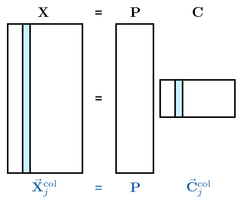
Figure 1: Illustration of solving $\mathbf{C}$ one column at a time, i.e., equation 13.

In equation 11, the $\vec{\phi}_{k}$ vectors are fixed and one solves the coefficients $c_{kj}$ with a separate set of equations for each observation $\vec{x}_{j}$. Written in matrix form, $\mathbf{X}=\mathbf{P}\mathbf{C}$ can be solved for each independent observation column $j$ of $\mathbf{X}$ and $\mathbf{C}$:

$$\vec{\mathbf{X}}^{\mathrm{col}}_{j}=\mathbf{P}\vec{\mathbf{C}}^{\mathrm{col}}_{j}+\mathrm{noise}$$ (13)

Equation 13 is illustrated in figure 1.

Solving equation 13 for $\vec{\mathbf{C}}^{\mathrm{col}}_{j}$ with noise-weighting by measurement covariance $\mathbf{V}_{j}$ is a straight-forward linear least-squares problem which may be solved with Singular Value Decomposition (SVD), QR factorization, conjugate gradients, or other methods. For example, using the method of “Normal equations” and the shorthand $\vec{x}=\vec{\mathbf{X}}^{\mathrm{col}}_{j}$ and $\vec{c}=\vec{\mathbf{C}}^{\mathrm{col}}_{j}$:

$$\vec{x} = \mathbf{P}\vec{c}$$ (14)

$$\mathbf{V}^{-1}\vec{x} = \mathbf{V}^{-1}\mathbf{P}\vec{c}$$ (15)

$$\mathbf{P}^{T}\mathbf{V}^{-1}\vec{x} = (\mathbf{P}^{T}\mathbf{V}^{-1}\mathbf{P})\vec{c}$$ (16)

$$(\mathbf{P}^{T}\mathbf{V}^{-1}\mathbf{P})^{-1}\mathbf{P}^{T}\mathbf{V}^{-1}\vec{x} = \vec{c}$$ (17)

If the noise is independent between variables, the inverse covariance $\mathbf{V}^{-1}$ is just a diagonal matrix of weights $\vec{\mathbf{W}}^{\mathrm{col}}_{j}$. Note that the covariance here is the estimated measurement covariance, not the total dataset variance — the goal is to weight the observations by the estimated measurement variance so that noisy observations do not unduly affect the solution, while allowing PCA to describe the remaining signal variance.

In the more general case of measurement covariance between different observations, one cannot solve equation 13 for each column of $\mathbf{X}$ independently. Instead, solve $\vec{\mathbf{X}}=[\mathbf{P}]\vec{\mathbf{C}}$ with the full covariance matrix $\mathbf{V}$ of $\vec{\mathbf{X}}$, where $[\mathbf{P}]$ is the matrix formed by stacking $\mathbf{P}$ $n_{\rm obs}$ times, and $\vec{\mathbf{X}}$ and $\vec{\mathbf{C}}$ are the vectors formed by stacking all the columns of the matrices $\mathbf{X}$ and $\mathbf{C}$. This requires the solution of a single $(n_{\rm obs}\cdot n_{\rm vec})\times(n_{\rm obs}\cdot n_{\rm vec})$ matrix rather than $n_{\rm obs}$ solutions of $n_{\rm vec}\times n_{\rm vec}$ matrices. If the individual observations are uncorrelated, it is computationally advantageous to use this non-correlation to solve multiple smaller matrices rather than one large one.

5.3.2 Notes on solving $\{\vec{\phi}_{k}\}=\mathbf{P}$

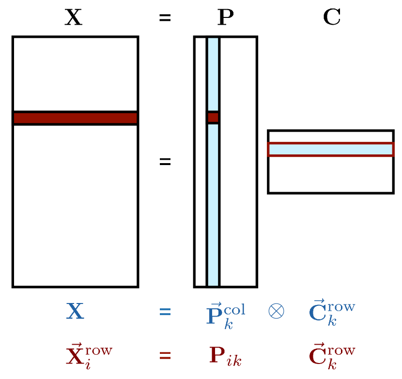
Figure 2: Illustration of solving $\mathbf{P}$ one element at a time, i.e., equation 20.

In the second step of each iteration (equation 12), we use the fixed coefficients $\mathbf{C}$ (dimensions $n_{\rm vec}\times n_{\rm obs}$) and solve for the eigenvectors $\mathbf{P}$ (dimensions $n_{\rm var}\times n_{\rm vec}$). We solve the eigenvectors one-by-one to maximize the power in each eigenvector before solving the next. Selecting out just the $k$th eigenvector uses the $k$th column of $\mathbf{P}$ and the $k$th row of $\mathbf{C}$:

$$\mathbf{X} = \vec{\mathbf{P}}^{\mathrm{col}}_{k}\otimes\vec{\mathbf{C}}^{\mathrm{row}}_{k}$$ (19)

where $\otimes$ signifies an outer product. If the variables (rows) of $\mathbf{X}$ are independent, then we can solve for a single element of $\vec{\mathbf{P}}^{\mathrm{col}}_{k}$ at a time:

$$\vec{\mathbf{X}}^{\mathrm{row}}_{i} = \mathbf{P}_{ik}\vec{\mathbf{C}}^{\mathrm{row}}_{k}$$ (20)

This is illustrated in figure 2. With independent weights $\vec{\mathbf{W}}^{\mathrm{row}}_{i}$ on the data $\vec{\mathbf{X}}^{\mathrm{row}}_{i}$, we solve variable $i$ of eigenvector $k$ with:

$$\mathbf{P}_{ik}={\sum_{j}\mathbf{W}_{ij}\mathbf{X}_{ij}\mathbf{C}_{ik}\over\sum_{j}\mathbf{W}_{ij}\mathbf{C}_{ik}\mathbf{C}_{ik}}$$ (21)

As with section 5.3.1, if there are measurement covariances between the data, equation 19 may be expanded to solve for all elements of $\vec{\mathbf{P}}^{\mathrm{col}}_{k}$ simultaneously using the full measurement covariance matrix of $\mathbf{X}$.

After solving for $\vec{\mathbf{P}}^{\mathrm{col}}_{k}$, subtract its projection from the data:

$$\mathbf{X}\leftarrow\mathbf{X}-\vec{\mathbf{P}}^{\mathrm{col}}_{k}\otimes\vec{\mathbf{C}}^{\mathrm{row}}_{k}$$ (22)

This removes any variation of the data in the direction of $\vec{\mathbf{P}}^{\mathrm{col}}_{k}$ so that additional eigenvectors will be orthogonal to the prior ones. Then repeat the procedure to solve for the next eigenvector $k+1$.

6 Extensions of Weighted EMPCA

The flexibility of the iterative EMPCA solution allows for a number of powerful extensions to PCA in addition to noise weighting. We describe a few of these here.

6.1 Smoothed EMPCA

If the length scale of the underlying signal eigenvectors is larger than that of the noise, it may be advantageous to smooth the eigenvectors to remove remaining noise effects. The iterative nature of EMPCA allows smoothing of the eigenvectors at each step to remove the high frequency noise. This generates the optimal smooth eigenvectors by construction rather than smoothing noisy eigenvectors afterward. This will be shown in the examples in section 7. Alternately, one can include a smoothing prior or regularization term when solving for the principal components $\mathbf{P}$. That approach, however, requires solving equation 19 (plus a regularization term) for all elements of $\vec{\mathbf{P}}^{\mathrm{col}}_{k}$ simultaneously instead of using the numerically much faster equation 21 for the case of diagonal measurement covariance.

6.2 A priori eigenvectors

In some applications, one has a few a priori template vectors to include in the fit, e.g., from some physical model. The goal is to find additional template vectors which are to be combined with the a priori vectors for the best fit of the data. Due to noise weighting and the potential non-orthogonality of the a priori vectors, the best fit is a joint fit and one cannot simply fit the a priori vectors and remove their components before proceeding with finding the other unknown vectors.

This case can be incorporated into EMPCA by including the a priori vectors in the starting vectors $\mathbf{P}$ and simply keeping them fixed with each iteration rather than updating them. In each iteration, the coefficients for the a priori vectors are updated, but not the vectors themselves.

7 Examples

7.1 Toy data

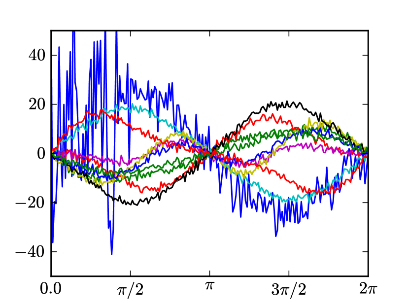
Figure 3: Example of noisy data used to test weighted EMPCA.

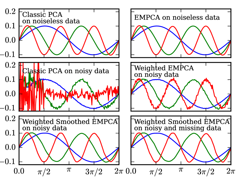
Figure 4: Examples of classic PCA and EMPCA applied to noiseless, noisy, and missing data.

Figure 3 shows example noisy data used to test weighted EMPCA. 100 data vectors were generated using 3 orthonormal sine functions as input, with random amplitudes drawn from Gaussian distributions. The lower frequency sine waves were given larger Gaussian sigmas such that they contribute more signal variance to the data. Gaussian random noise was added, with 10% of the data vectors receiving 25 times more noise from [0, $\pi/2$] and 5 times more noise from [$\pi/2$, $2\pi$]. For Weighted EMPCA, weights were assigned as $1/\sigma^{2}$, where $\sigma$ is the per-observation per-variable Gaussian sigma of the added noise (not the sigma of the underlying signal). A final dataset was created where a contiguous 10% of each observation was set to have weight=0 to create regions of missing data. As a crosscheck that the 0 weights are correctly applied, the data in these regions were set to a constant value of 1000 – if these data are not correctly ignored by the algorithm they will have a large effect on the extracted eigenvectors.

Figure 4 show the results of applying classic PCA and weighted EMPCA to these data. Upper left: Classic PCA applied to the noiseless data recovers the input eigenvectors, slightly rotated to form the best ranked eigenvectors for describing the data variance. Upper right: EMPCA applied to the same noiseless data recovers the same input eigenvectors. Middle left: When classic PCA is applied to the noisy data, the highest order eigenvector is dominated by the noise, and the effects of the non-uniform noise are clearly evident as increased noise from [0, $\pi/2$]. Middle right: Weighted EMPCA is much more robust to the noisy data, extracting results close to the original eigenvectors. The highest order eigenvector is still affected by the noise, which is a reflection that the noise does contribute power to the data variance. However, the extra-noisy region from [0, $\pi/2$] is not affected more than the region from [$\pi/2$, $2\pi$], due to the proper deweighting of the noisy data. Lower left: Smoothed weighted EMPCA is almost completely effective at extracting the original eigenvectors with minimal impact from the noise. Lower right: Even when 10% of every observation is missing, smoothed weighted EMPCA is effective at extracting the underlying eigenvectors. All eigenvectors for all methods are orthogonal at the level of ${\cal O}(10^{-17})$.

7.2 QSO data

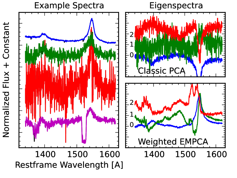
Figure 5: Example of high-, median-, and low-$S/N$ input QSO spectra and a broad absorption line (BAL) QSO (left). The first 3 classic PCA eigenvectors are shown at top right; the first 3 weighted EMPCA eigenvectors are shown at bottom right.

Figure 5 shows the results of applying classic PCA and weighted EMPCA to QSO spectra from the Sloan Digital Sky Survey Data Release 7 (Abazajian et al., 2009), using the QSO redshift catalog of Hewett & Wild (2010). 500 spectra of QSOs with redshift $2.0<z<2.1$ were randomly selected and trimmed to $1340<\lambda<1620$ Å to show the SiIV and CIV emission features. Spectra with more than half of the pixels masked were discarded. Each spectrum was normalized to median[flux($1440<\lambda<1500$ Å)] $=1$ and the weighted mean of all normalized spectra was subtracted. The left panel of Fig. 5 plots examples of high, median, and low signal-to-noise spectra and a broad absorption line (BAL) QSO from this sample. $\sim$2% of the spectral bins have been flagged with a bad-data mask, e.g., due to cosmic rays, poor sky subtraction, or the presence of non-QSO narrow absorption features from the intergalactic medium. These are treated as missing data with weight=0. The goal of weighted EMPCA is to properly deweight the noisy spectra such that the resulting eigenvectors are predominantly describing the underlying signal variations and not just measurement noise. Weights are $1/\sigma_{ij}^{2}$ where $\sigma_{ij}$ is the SDSS pipeline estimated measurement noise for wavelength bin $i$ of spectrum $j$. Weighted EMPCA can also properly ignore the masked data by using weight=0 without having to discard the entire spectrum, or artificially interpolate over the masked region.

The right panels of Fig. 5 show the results for the first 3 eigenvectors of classic PCA (top right) and weighted EMPCA (bottom right). Eigenvectors 0, 1, and 2 are plotted in blue, green, and red respectively. The mean spectrum was subtracted prior to performing PCA such that these eigenvectors represent the principal variations of the spectra with respect to that mean spectrum. Eigenvectors are orthogonal at the level of ${\cal O}(10^{-17})$.

The EMPCA eigenvectors are much less noisy than the classic PCA eigenvectors. As such, they are more sensitive to genuine signal variations in the data. For example, the sharp features between $1515<\lambda<1545$ Å in the EMPCA eigenspectra arise from BAL QSOs, an example of which is shown in the bottom of the left panel of Fig. 5. These features are used to study QSO outflows, e.g. Turnshek (1988), yet they are lost amidst the noise of the classic PCA eigenspectra. Similarly, the EMPCA eigenspectra are more sensitive to the details of the variations in shape and location of the emission peaks used to study QSO metallicity (e.g. Juarez et al. (2009)) and black hole mass (e.g. Vestergaard & Osmer (2009)).

8 Discussion

8.1 Convergence

McLachlan & Krishnan (1997) discuss the convergence properties of the EM algorithm in general. Each iteration, by construction, finds a set of parameters that are as good or better a fit to the data than the previous step, thus guaranteeing convergence. The caveat is that the “Likelihood maximization step” is typically implemented as solving for a stationary point of the likelihood surface rather than strictly a maximum. e.g., $\partial{\cal L}/\partial\phi=0$ is also true at saddle points and minima of the likelihood surface, thus it is possible that the EM algorithm will not converge to the true global maximum. Unweighted PCA has a likelihood surface with a single global maximum, but in general this is not the case for weighted PCA: the weights in equation 8 can result in local false $\chi^{2}$ minima (Srebro & Jaakkola, 2003). McLachlan & Krishnan (1997) §3.6 also gives examples of this behavior (taken from Murray (1977) and Arslan, Constable, & Kent (1993)) for the closely related problem of Factor Analysis. The example datasets are somewhat contrived and the minimum or saddle point convergence only happens with particular starting conditions.

We have encountered false minima with weighted EMPCA when certain observations have $\sim$90% of their variables masked while giving large weight to their remaining unmasked variables. In this case the resultant eigenvectors can have artifacts tuned to the highly weighted but mostly masked input observations. When only a few ($\sim$10%) of the variables are masked per observation, we have not had a problem with false minima.

The algorithm outlined in section 5 solves for each eigenvector one at a time in order to maximize the power in the initial eigenvectors. This can result in a situation where a given iteration can improve the power described by the first few eigenvectors while degrading the total $\chi^{2}$ using all eigenvectors. We have not found a case where this significantly degrades the global $\chi^{2}$, however.

The speed of convergence is also not guaranteed. Roweis (1997) gives a toy example of fast convergence for Gaussian-distributed data (3 iterations), and slow convergence for non-Gaussian-distributed data (23 iterations). In practice we find that when EMPCA is slow to converge, it is exploring a shallow likelihood surface between two nearly degenerate eigenvectors. This situation pertains to the uniqueness of the solution, described in the following section.

Weighted EMPCA may produce unstable solutions if it is used to solve for more eigenvectors than are actually present in the data, or for eigenvectors that are nearly singular. Since EMPCA uses all eigenvectors while solving for the coefficients during each iteration, the singular eigenvectors can lead to delicately balanced meaningless values of the coefficients, which in turn degrades the solution of the updated eigenvectors in the next iteration. We recommend starting with solving for a small number of eigenvectors, and then increasing the number of eigenvectors if the resulting solution does not describe enough of the data variance.

For these reasons, one should use caution when analyzing data with EMPCA, just as one should do with any problem which is susceptible to false minima or other convergence issues. In practice, we find that the benefits of proper noise-weighting outweigh the potential convergence problems.

8.2 Uniqueness

Given that EMPCA is an iterative algorithm with a random starting point, the solution is not unique. In particular, if two eigenvalues are very close in magnitude, EMPCA could return an admixture of the corresponding eigenvectors while still satisfying the convergence criteria. In practice, however, EMPCA is pragmatic: if two eigenvectors have the same eigenvalue, they are also equivalently good at describing the variance in the data and could be used interchangeably.

Science applications, however, generally require strict algorithmic reproducibility and thus EMPCA should be used with a fixed random number generator seed or fixed orthonormal starting vectors such as Legendre polynomials. The convergence criteria define when a given vector is “good enough” to move on to the next iteration, but they do not guarantee uniqueness of that vector.

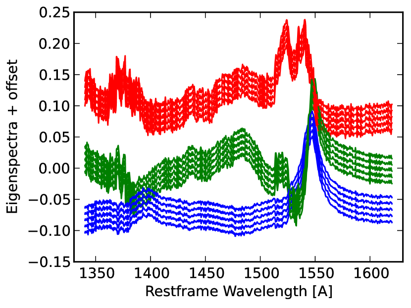
Figure 6: Example eigenspectra of the same dataset with different random starting values for the EMPCA algorithm. The eigenspectra are offset for clarity and have bin-for-bin agreement at the level of $\sim$10^-5.

Figure 6 shows the first 3 eigenvectors for 5 different EMPCA solutions of the QSO spectra from section 7.2 with different random starting vectors. After 20 iterations the eigenvectors agree to $<10^{-5}$ on both large and small scales. Although this agreement is worse than the machine precision of the computation, it is much smaller than the scale of differences between the eigenvectors and it represents a practical level of convergence for most PCA applications.

8.3 Over-weighted Data

Weighted EMPCA improves the PCA eigenvector solution by preventing noisy or missing data from unduly contributing noise instead of signal variation. However, the opposite case of high signal-to-noise data can also be problematic if just a few of the observations have significantly higher weight than the others. These will dominate the EMPCA solution just as they would dominate a weighted mean calculation. This may not be the desired effect since the initial eigenvectors will describe the differences between the highly weighted data and subsequent eigenvectors will describe the lower weighted data. This may be prevented by purposefully down-weighting certain observations or applying an upper limit to weights so that the weighted dataset isn’t dominated by just a few observations.

8.4 Scaling Performance

The primary advantage of EMPCA is the ability to incorporate weights on noisy data to improve the quality of the resulting eigenspectra. A secondary benefit over classic PCA is algorithmic speed for the common case of needing only the first few eigenvectors from a dataset with $n_{\rm obs}\stackrel{{\scriptstyle<}}{{\sim}}n_{\rm var}$.

Classic PCA requires solving the eigenvectors of the data covariance matrix, an ${\cal O}(n_{\rm var}^{3})$ operation. The weighted EMPCA algorithm described here involves iterating over multiple solutions of smaller matrices. Each iteration requires $n_{\rm obs}$ solutions of ${\cal O}(n_{\rm vec}^{3})$ to solve the coefficients and ${\cal O}(n_{\rm obs}n_{\rm vec}n_{\rm var})$ operations to solve the eigenvectors. Thus weighted EMPCA can be faster than classic PCA when $n_{\mathrm{iter}}(n_{\rm obs}n_{\rm vec}^{3}+n_{\rm obs}n_{\rm vec}n_{\rm var})<n_{\rm var}^{3}$, ignoring the constant prefactors. If one has a few hundred spectra ($n_{\rm obs}$) with a few thousand wavelengths each ($n_{\rm var}$) and wishes to solve for the first few eigenvectors ($n_{\rm vec}$), then EMPCA can be much faster than classic PCA. Conversely, if one wishes to perform PCA on all $\sim$1 million spectra from SDSS, then $n_{\rm obs}\gg n_{\rm var}$ and classic PCA is faster, albeit with the limitations of not being able to properly weight noisy or missing data. If the problem involves off-diagonal covariances, then weighted EMPCA involves a smaller number of larger matrix solutions for an overall slowdown, though note that classic PCA is unable to properly solve the problem at all.

As a performance example, we used EMPCA to study the variations in the simulated point spread function (PSF) of a new spectrograph design. The PSFs were simulated on a grid of 11 wavelengths and 6 slit locations, and were sampled over $200\times 200$ $\mu$m spots on a 1 $\mu$m grid, for a total of 40000 variables per spot. Classic PCA would require singular value decomposition of a $40000\times 40000$ matrix. While this is possible, it is beyond the scope of a typical laptop computer. On the other hand, using EMPCA with constant weights we were able to recover the first 30 eigenvectors covering 99.7% of the PSF variance in less than 6 minutes on a 2.13 GHz MacBook Air laptop.

For datasets where $n_{\rm var}$ is particularly large, the memory needed to store the $n_{\rm var}\times n_{\rm var}$ covariance matrix may be a limiting factor for classic PCA. The iterative nature of EMPCA allows one to scale to extremely large datasets since one never needs to keep the entire dataset (nor its covariance) in memory at one time. The multiple independent equations to solve in sections 5.3.1 and 5.3.2 are naturally computationally parallelizable.

9 Python Code

Python code implementing the Weighted EMPCA algorithm described here is available at https://github.com/sbailey/empca . The current version implements the case of independent weights but not the more generalized case of off-diagonal covariances. It also implements the smoothed eigenvectors described in §6.1, but not a priori eigenvectors (§6.2), nor distributed calculations (§8.4). For comparison, the empca module also includes implementations of classic PCA and weighted lower-rank matrix approximation. Examples for this paper were prepared with tagged version v0.2 of the code.

When using the code, note that the orientation of the data and weights vectors is the transpose of the notation used here, i.e., data[j,i] is variable i of observation j so that data[j] is a single observation.

10 Summary

To briefly summarize the algorithm: A data matrix $\mathbf{X}$ can be approximated by a set of eigenvectors $\mathbf{P}$ with coefficients $\mathbf{C}$:

$$\mathbf{X}\approx\mathbf{P}\mathbf{C}+\mathrm{measurement~{}noise}$$ (23)

A covariance matrix $\mathbf{V}$ describes the estimated measurement noise.

The Weighted EMPCA algorithm seeks to find the optimal $\mathbf{P}$ and $\mathbf{C}$ given $\mathbf{X}$ and $\mathbf{V}$. It starts with a random set of orthonormal vectors $\mathbf{P}$, and then iteratively alternates solutions for $\mathbf{C}$ given $\{\mathbf{P},\mathbf{X},\mathbf{V}\}$ and $\mathbf{P}$ given $\{\mathbf{C},\mathbf{X},\mathbf{V}\}$. The problem is additionally constrained by the requirement to maximize the power in the fewest number of eigenvectors (columns of $\mathbf{P}$). To accomplish this, the algorithm solves for each eigenvector individually, before removing its projection from the data and solving for the next eigenvector. If the measurement errors are independent, the covariance can be described by a weights matrix $\mathbf{W}$ with the same dimensions as $\mathbf{X}$, and the problem can be factorized into independent solutions of small matrices.

This algorithm produces a set of orthogonal principal component eigenvectors $\mathbf{P}$, which are optimized to describe the most signal variance with the fewest vectors while properly accounting for estimated measurement noise.

11 Conclusions

We have described a method for performing PCA on noisy data that properly incorporates measurement noise estimates when solving for the eigenvectors and coefficients. Missing data is simply the limiting case of weight=0. The method uses an iterative solution based upon Expectation Maximization. The resulting eigenvectors are less sensitive to measurement noise and more sensitive to true underlying signal variations. The algorithm has been demonstrated on toy data and QSO spectra from SDSS. Code which implements this algorithm is available at https://github.com/sbailey/empca .

12 Acknowledgements

The author would like to thank Rollin Thomas and Sébastien Bongard for interesting and helpful conversations related to this work. The anonymous reviewer provided helpful comments and suggestions which improved this manuscript. The initial algorithm was developed during a workshop at the Institut de Fragny. This work was supported under the auspices of the Office of Science, U.S. DOE, under Contract No. DE-AC02-05CH1123.

The example QSO spectra were provided by the Sloan Digital Sky Survey. Funding for the SDSS and SDSS-II has been provided by the Alfred P. Sloan Foundation, the Participating Institutions, the National Science Foundation, the U.S. Department of Energy, the National Aeronautics and Space Administration, the Japanese Monbukagakusho, the Max Planck Society, and the Higher Education Funding Council for England. The SDSS Web Site is http://www.sdss.org/.

The SDSS is managed by the Astrophysical Research Consortium for the Participating Institutions. The Participating Institutions are the American Museum of Natural History, Astrophysical Institute Potsdam, University of Basel, University of Cambridge, Case Western Reserve University, University of Chicago, Drexel University, Fermilab, the Institute for Advanced Study, the Japan Participation Group, Johns Hopkins University, the Joint Institute for Nuclear Astrophysics, the Kavli Institute for Particle Astrophysics and Cosmology, the Korean Scientist Group, the Chinese Academy of Sciences (LAMOST), Los Alamos National Laboratory, the Max-Planck-Institute for Astronomy (MPIA), the Max-Planck-Institute for Astrophysics (MPA), New Mexico State University, Ohio State University, University of Pittsburgh, University of Portsmouth, Princeton University, the United States Naval Observatory, and the University of Washington.

References

- Abazajian et al. (2009) Abazajian, K. N., Adelman-McCarthy, J. K., Agüeros, M. A., et al. 2009, ApJS, 182, 543
- Arslan, Constable, & Kent (1993) Arslan, O., Constable, P.D.L., and Kent, J.T., 1993, Statistics and Computing, 3, 103–108.
- Blanton & Roweis (2007) Blanton, M. R., & Roweis, S. 2007, AJ, 133, 734
- Bond (1995) Bond, J. R. 1995, Physical Review Letters, 74, 4369
- Connolly & Szalay (1999) Connolly, A. J., & Szalay, A. S. 1999, AJ, 117, 2052
- Dempster, Laird, & Rubin (1977) Dempster, A.P., Laird, N.M., and Rubin, D.B. (1977). J. R. Statist. Soc. B, 39, 1–-38
- Gabriel & Zamir (1979) Gabriel, K.R., & Zamir, S. 1979, Technometrics, 21 489–498
- Hewett & Wild (2010) Hewett, P. C., & Wild, V. 2010, MNRAS, 405, 2302
- Hotelling (1933) Hotelling, H. 1933, J. Educ. Psychol., 24, 417–441
- Jee et al. (2007) Jee, M. J., Blakeslee, J. P., Sirianni, M., et al. 2007, PASP, 119, 1403
- Jolliffe (2002) Jolliffe, I.T. 2002, “Principal Component Analysis, Second Edition”, Springer, New York
- Juarez et al. (2009) Juarez, Y., Maiolino, R., Mujica, R., et al. 2009, A&A, 494, L25