Transition dynamics in aging systems: microscopic origin of logarithmic time evolution

Abstract

There exists compelling experimental evidence in numerous systems for logarithmically slow time evolution, yet its theoretical understanding remains elusive. We here introduce and study a generic transition process in complex systems, based on non-renewal, aging waiting times. Each state $n$ of the system follows a local clock initiated at $t=0$. The random time $\tau$ between clock ticks follows the waiting time density $\psi(\tau)$. Transitions between states occur only at local clock ticks and are hence triggered by the local forward waiting time, rather than by $\psi(\tau)$. For power-law forms $\psi(\tau)\simeq\tau^{-1-\alpha}$ ($0<\alpha<1$) we obtain a logarithmic time evolution of the state number $\langle n(t)\rangle\simeq\log(t/t_{0})$, while for $\alpha>2$ the process becomes normal in the sense that $\langle n(t)\rangle\simeq t$. In the intermediate range $1<\alpha<2$ we find the power-law growth $\langle n(t)\rangle\simeq t^{\alpha-1}$. Our model provides a universal description for transition dynamics between aging and non-aging states.

Imagine that you put a thin sheet of paper in a vertical cylinder and let the paper crumple under a heavy piston. If during compression you measure the piston’s velocity you will notice that it decreases over time, well in accordance with your intuition. However, what may appear surprising is that the piston keeps compressing the paper and never seems to come to a full rest. The outcome of such an experiment was reported by Matan et al. matan2001crumpling , concluding that the piston’s position $z(t)$ at long times $t$ decreases logarithmically, $z(t)\sim a-b\log(t/{\sec})$, where $a$ and $b$ are constants. The crumpling of paper is by far the only example for logarithmically slow dynamics. It is observed in DNA local structure relaxation brauns2002complex , the time evolution of frictional strength ben2010slip , compactification of grains by tapping richard2005slow , kinetics of amorphous-amorphous transformations in glasses under high pressure tsiok1998logarithmic , magnetisation dynamics in high-$T_{c}$ superconductors gurevich1993time , conductance relaxations amir2012relaxations ; amir2011huge and current relaxation in semiconductor field-effect transistors woltjer1993time . Other examples of logarithmic time evolution include decays in colloidal systems sperl2003 , aging in simple glasses angelani01 (see also Supplementary Material supp ), magnetisation relaxation in spin glasses chowdhury1984logarithmic , evolution of node connectivity in a network with uniform attachment barabasi1999 , diffusion in a random force landscape (Sinai diffusion) havlin2002 , and record statistics zia1999 .

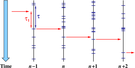
Figure 1: Dynamic update of successive states. At each state $n$, a tick of the local clock allows the transition to the next state, $n+1$. Local clock ticks are separated by waiting times $\tau$ drawn from the distribution $\psi(\tau)$. After transition from state $n-1$ the system is locked in $n$ until the next clock tick at $n$, after the forward waiting time $\tau_{1}<\tau$. Typically a transition at a new state arrives during a long waiting time, the statistics of the $\tau_{1}$ thus slowing down the overall dynamics.

Here we introduce a generic microscopic model displaying logarithmic time evolution which is based on non-renewal sequential transitions between aging states labeled ny $n$ (see Fig. 1). As we show analytically, the $q$th order moments of the resulting counting process at large times grow as

$$\langle n^{q}(t)\rangle\sim\left[\frac{\ln(t/t_{0})}{\mu}\right]^{q}\left\{1+\frac{q}{2}\left[\frac{q\sigma^{2}}{\mu}-\mu\right]\frac{1}{\ln(t/t_{0})}\right\}$$ (1)

such that, particularly, we find the logarithmically slow counting process $\langle n(t)\rangle\simeq\log(t/t_{0})$. The parameters $\mu$ and $\sigma$ depend on the details of the underlying dynamics and are specified below, and $t_{0}$ is the time when the counting started after global system initiation at $t=0$, for instance, by an external perturbation. We also show that under non-aging conditions our model leads to the expected linear growth $\langle n(t)\rangle\simeq t$, and in the intermediate case we observe power-law scaling for $\langle n(t)\rangle$. Our model provides an intuitive mesoscopic approach to the superslow dynamics in aging systems.

We define the dynamics of the system through a series $n(t)$ of consecutive states, each of which is characterized by its own local clock and all being initiated globally at time $t=0$. The clocks’ ticks occur with random time intervals $\tau$, which are drawn from a waiting time density $\psi(\tau)$ (see Fig. 1). If the system arrives at state $n-1$ at a later time $t^{\prime}$ then it is more likely to a encounter a large $\tau$, and therefore also typically has to wait a correspondingly longer time $\tau_{1}$ before a transition to state $n$ occurs. For $\psi(\tau)\simeq\tau^{-1-\alpha}$ with $0<\alpha<1$, no typical time scale $\langle\tau\rangle=\int_{0}^{\infty}\tau\psi(\tau)d\tau$ exists, and we find Eq. (1), whose scaling with the counting initiation time $t_{0}$ manifests the aging property of the process REMM . Equation (1) is the central result of this work, but we also obtain $\langle n^{q}(t)\rangle$ for $\alpha>1$. Moreover, we find the probability distribution $h_{n}(t)$ to be in state $n$ at time $t$ given that the counting of transitions (from state $0$) began at $t=t_{0}$.

A simplistic picture for our model is to envision a hitchhiker traveling through a series of towns. In each town, traffic starts in the morning, and friendly drivers (persons willing to pick up our hitchhiker) appear at random intervals $\tau$ governed by $\psi$. The hitchhiker typically arrives to a new town in between two friendly drivers show up, and the delay time $\tau_{1}$, i.e. the time the hitchhiker actually has to wait until the next ride, is governed by the forward waiting time density $\psi_{1}$ REM . The probability density $\psi_{1}$ is far from trivial: for heavy-tailed $\psi(\tau)$ it displays aging, see below. In this context it is interesting to note that indeed arrival times of English trains, but also response times in human communication patterns, and bursting in queuing models are power-law distributed REMMM ; oliveira2005human ; barabasi2005origin .

A more physical picture for our model is defect-mediated crack-type propagation in a solid. Imagine a crack that grows in discrete steps ($...,n-1,n,...$), the growth being triggered by the arrival of a diffusing defect at the neighbouring site of the crack’s tip, similar in spirit to Glarum’s defect diffusion model glarum . The global initiation in this system occurs when the external stress is applied. Possibly, similar scenarios may apply in the above-mentioned examples of stick-slip dynamics ben2010slip and density relaxation of grains by tapping richard2005slow .

We now formulate our process mathematically. To that end we define the probability density $\rho_{n}(t)$ for the system to arrive at state $n$ at time $t$, which fulfils the convolution

$$\rho_{n}(t)=\int_{0}^{t}\rho_{n-1}(t^{\prime})\psi_{1}(t-t^{\prime}|t^{\prime})dt^{\prime},\,\,\rho_{0}(t)=\delta(t-t_{0}),$$ (2)

where $\psi_{1}(\tau_{1}|t^{\prime})$ is the probability density of the triggering delay time (forward waiting time) $\tau_{1}$ that the system spends in a new state after having arrived there at time $t^{\prime}$. Equation (2) expresses the fact that the probability to arrive at state $n$ in a time interval $[t,t+dt]$ is the probability of having arrived to the state $n-1$ at some earlier time interval $[t^{\prime},t^{\prime}+dt^{\prime}]$ ($t^{\prime}<t$) multiplied by the probability of a triggering event occurring in $[t^{\prime},t^{\prime}+dt^{\prime}]$, where $t^{\prime}$ lies anywhere between 0 and $t$. Now, if $\psi(\tau)\simeq\tau^{-1-\alpha}$ with $0<\alpha<1$ ($\alpha>1$ is discussed below) then the probability density $\psi_{1}$ of forward waiting times $\tau_{1}$ is known from continuous time random walk (CTRW) theory, namely dynkin ; godreche ; koren

$$\psi_{1}(\tau_{1}|t^{\prime})=\frac{\sin(\pi\alpha)}{\pi}\frac{{t^{\prime}}^{\alpha}}{\tau_{1}^{\alpha}(t^{\prime}+\tau_{1})}.$$ (3)

This quantity explicitly depends on the arrival time $t^{\prime}$ and thus mirrors the aging property of the process: while at small $t^{\prime}$, we observe the scaling $\psi_{1}\simeq\tau_{1}^{-1-\alpha}$ in analogy to the regular waiting time density $\psi(\tau)$, at longer $t^{\prime}$ we have to wait for a longer $\tau_{1}$ for the next transition event. This intuitively corresponds to the observation of a random walk process governed by the waiting time density $\psi(\tau)\simeq\tau^{-1-\alpha}$ with $0<\alpha<1$: when the process evolves (i.e., becomes older), due to the scale-free nature of $\psi$ we see increasingly longer waiting times. The later we arrive at a new state (growing $t^{\prime}$), the longer will the current tick-tick waiting time $\tau$ be and thus $\tau_{1}$ grows longer as the overall process develops.

We note that our model is in stark contrast with standard CTRW theory where the waiting time is reset (renewed) after each transition report ; scher , i.e., the renewals are an intrinsic property of the process. Here we update each state locally starting at $t=0$, and each local clock is renewed after a tick. However, the overall process effectively couples all the local clocks, since after a transition to a new state $n$ (i.e., a tick at state $n-1$) the process needs to wait for the next local tick (at $n$). This bestows the non-renewal property of the overall process.

Finally, we obtain the probability $h_{n}(t)$ to find the system in state $n$ at time $t$. It corresponds to the probability of having arrived at $n$ at $t^{\prime}<t$, and no transition having occurred since:

$$h_{n}(t)=\int_{0}^{t}\rho_{n}(t^{\prime})\int_{t-t^{\prime}}^{\infty}\psi_{1}(\tau_{1}|t^{\prime})d\tau_{1}dt^{\prime}.$$ (4)

Eqs. (2) to (4) define the problem we solve here.

To proceed it is convenient to employ the technique of Mellin transforms davies2002 . With $G(x)\equiv x\psi_{1}(x-1|1)\theta(x-1)$, where $\theta(x)$ is the unit step function, Eq. (2) becomes

$$\rho_{n}(t)=\frac{1}{t}\int_{0}^{\infty}\rho_{n-1}(t^{\prime})G(t/t^{\prime})dt^{\prime}.$$ (5)

Using the definition of Mellin transforms $f(p)=\int_{0}^{\infty}t^{p-1}f(t)dt$, where $p$ is the Mellin variable, along with the Mellin convolution theorem davies2002 we obtain from Eq. (5) that $\rho_{n}(p)=G(p-1)\rho_{n-1}(p)$, to which the solution is $\rho_{n}(p)=[G(p-1)]^{n}t_{0}^{p-1}$ [here we used $\rho_{0}(p)=t_{0}^{p-1}$]. The Mellin transform of Eq. (4) is $h_{n}(p)=\rho_{n}(p+1)[G(p)-1]/p$, and therefore

$$h_{n}(p)=t_{0}^{p}G(p)^{n}[G(p)-1]/p.$$ (6)

This is an exact solution in Mellin space for the sought-after quantity $h_{n}(t)$ used in the following.

While no simple expression exists for the exact $h_{n}(t)$ we can obtain all moments of $h_{n}(t)$ in the limit of long times $t$. Expanding $G(p)$ for small $p$ to second order, for $0<\alpha<1$, we obtain the $q$th order moments supp

$$\langle n^{q}(p)\rangle\sim\frac{\Gamma(q+1)t_{0}^{p}}{\mu^{q}(-p)^{q+1}}\left\{1+\frac{p}{2}\left[\mu-q\sigma^{2}/\mu\right]\right\},\,\,\,p\to 0^{-}$$ (7)

in Mellin space, with $\mu=-\Gamma^{\prime}(\alpha)/\Gamma(\alpha)-\gamma$ and $\sigma^{2}=-\pi^{2}/6+\partial^{2}\ln\Gamma(\alpha)/\partial\alpha^{2}$. Here, $\Gamma(z)$ is the complete $\Gamma$ function, and $\gamma=0.5772..$ denotes Euler’s constant. Inverting the Mellin transform, we retrieve Eq. (1) at long $t$. Thus the leading order behavior of the first two moments follows $\langle n(t)\rangle\sim\ln(t/t_{0})/\mu$ and $\langle n^{2}(t)\rangle\sim\ln^{2}(t/t_{0})/\mu^{2}$. This shows that the triggering process considered here leads to a non-trivial logarithmic time evolution for heavy-tailed forms of $\psi(\tau)$. The logarithmically slow dynamics contrasts the case $\alpha>1$ for which $\langle n^{q}(t)\rangle$ grows as a power-law (shown below). In Fig. 2 we compare our analytical result (7) for $\langle n(t)\rangle$ with simulations REM1 for the concrete form $\psi(\tau)=\alpha\tau_{0}^{\alpha}/(\tau+\tau_{0})^{1+\alpha}$. As can be seen, the simulations agree excellently with Eq. (1), except for $\alpha\to 1$. The inset of Fig. 2 shows that the mismatch is due to the fact that $t_{0}$ is not sufficiently large (i.e., not much larger than $\tau_{0}$) and the distribution $\psi_{1}(\tau_{1}|t_{0})$ thus has not reached its asymptotic form (3).

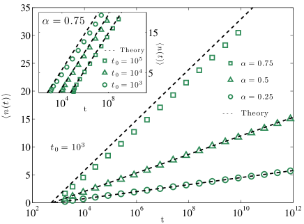
Figure 2: Average state number $\langle n(t)\rangle$ versus time $t$. Symbols represent simulations for various $\alpha$, as indicated. Dashed lines show the asymptotic behavior, Eq. (1) for $q=1$. In the simulations we used $t_{0}=10^{3}$ and $\tau_{0}=1$. Results are ensemble averaged over $10^{7}$ runs, respectively. Inset: convergence to the theoretical results with $t_{0}$ for $\alpha=0.75$.

The $q$-dependence of the dominant term in Eq. (1) corresponds to a $\delta$-function for the limiting distribution. This means that the standard deviation versus the mean in our model becomes increasingly small for long times and that the dynamics becomes effectively deterministic. Indeed, dividing the variance by the mean we find

$$\frac{\sqrt{\langle n^{2}(t)\rangle-\langle n(t)\rangle^{2}}}{\langle n(t)\rangle}\sim\sqrt{\frac{\sigma^{2}}{\mu\ln(t/t_{0})}},$$ (8)

as is nicely corroborated by simulations of this ratio in Fig. 3. Equation (8) contrasts the behavior of the position coordinate in biased subdiffusive CTRW processes where the ratio above tends to a constant scher .

What about the behavior when $\alpha>1$? In this case $\psi_{1}(\tau_{1}|t^{\prime})$ has a finite limit independent of $t^{\prime}$ and is given by $\psi_{1}(\tau_{1})=\int_{\tau_{1}}^{\infty}\psi(\tau^{\prime})d\tau^{\prime}/\langle\tau\rangle$ klaso , where $\langle\tau\rangle=\int_{0}^{\infty}\tau\psi(\tau)d\tau$. Assuming the form $\psi(\tau)\sim A/\tau^{\alpha+1}$ for large $\tau$ one obtains $\psi_{1}(\tau_{1})\sim(\alpha-1)A/[\langle\tau\rangle\tau_{1}^{\alpha}]$. We find two distinct regimes for the cases $1<\alpha<2$ and $\alpha>2$. For $1<\alpha<2$ the system goes through the series of states, $n(t)$, as a regular renewal process with power-law waiting times of index $\alpha-1$. The number of states the system passes in this case thus has the moments koren ; REM2

$$\langle n^{q}(t)\rangle\sim\frac{\Gamma(q+1)}{\Gamma(q(\alpha-1)+1)}\left(\frac{\langle\tau\rangle t^{\alpha-1}}{\Gamma(2-\alpha)A}\right)^{q}\propto t^{(\alpha-1)q}.$$ (9)

Here we notice that the mean $\langle n(t)\rangle\simeq t^{\alpha-1}$ increases sublinearly rather than logarithmically as in the case $0<\alpha<1$. Moreover, we find that the fluctuations grow as fast as the mean. For $\alpha>2$ we put $\alpha\to 2$ and $\Gamma(2-\alpha)A\to\langle\tau^{2}\rangle/2$ so that we obtain

$$\langle n^{q}(t)\rangle\sim\left(\frac{2\langle\tau\rangle t}{\langle\tau^{2}\rangle}\right)^{q}\propto t^{q}.$$ (10)

In this case, in particular, the mean grows linearly with time. Interestingly, just as for the case $0<\alpha<1$ (but in contrast to the regime $1<\alpha<2$), the deviations vanish relative to the mean, i.e., the long-time dynamics is effectively deterministic.

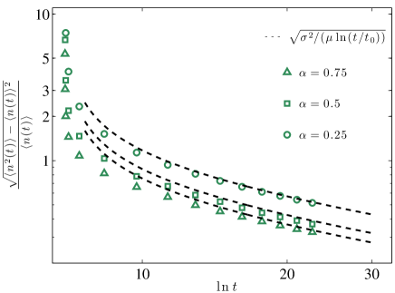
Figure 3: Standard deviation versus mean as a function of process time. Simulations (symbols) are compared to the asymptotic results for large $t$ [Eq. (8), dashed lines]. Parameters used: $t_{0}=10^{3}$, $\tau_{0}=1$, averaged over $7\times 10^{5}$ simulation runs.

We now turn our attention to the full distribution $h_{n}(t)$ for the case $0<\alpha<1$. To that end we need to evaluate the inverse Mellin transform of Eq. (6). In the Supplementary Material supp we derive the approximate form

$$h_{n}^{(1)}(t)=h_{n}^{(0)}(t)\left[1+\frac{\sigma^{2}+\mu^{2}}{2\mu\sqrt{\sigma^{2}n}}y+\frac{\kappa_{3}n}{6(\sigma^{2}n)^{3/2}}(y^{3}-3y)\right],$$ (11)

where $y=[\ln(t/t_{0})-\mu n]/\sqrt{\sigma^{2}n}$ and

$$h^{(0)}_{n}(t)=\frac{\mu}{\sqrt{2\pi\sigma^{2}n}}\exp\left(-\frac{(\ln(t/t_{0})-\mu n)^{2}}{2\sigma^{2}n}\right).$$ (12)

The distribution $h_{n}(t)$, for fixed (logarithmic) time, is thus a slightly skewed Gaussian in the $n$-domain. In Fig. 4 we compare the result $h_{n}^{(1)}(t)$ with simulations, demonstrating good agreement for its dominating part.

Figure 4: Probability distribution to find the system in state $n$ at time $t$. Lines: analytical results from Eqs. (11) and (12). Circles: simulation results, averaged over $7\times 10^{5}$ runs. Parameters used: $t=7.9\times 10^{12}$, $t_{0}=10^{3}$, $\tau_{0}=1$, and $\alpha=0.25$.

In particle tracking assays single trajectories are routinely measured and analysed pt . We therefore also consider the time average for a single realization of $n(t)$ defined as $\overline{n(\Delta)}=(t_{2}-\Delta-t_{1})^{-1}\int_{t_{1}}^{t_{2}-\Delta}[n(t+\Delta)-n(t)]dt$, where the observation time of the trajectory is from $t_{1}$ to $t_{2}$, and $\Delta$ is the lag time. Here we only consider the heavy-tailed case $0<\alpha<1$. Averaging over many trajectories, the dominant behavior at $t_{1},t_{2}\gg t_{0}$ becomes

$$\left<\overline{n(\Delta)}\right>\sim\Delta\frac{1/\mu}{t_{2}-t_{1}}\ln\frac{t_{2}}{t_{1}}$$ (13)

for $\Delta\ll t_{2}-t_{1}$. The linear behavior in $\Delta$ contrasts the logarithmic time dependence of $\langle n(t)\rangle$. This discrepancy between ensemble and time average demonstrates that the process considered here is weakly non-ergodic pt ; bouchaud92 ; bel07 . Interestingly, while the duration $t_{2}-t_{1}$ and the aging time $t_{1}$ factorize from the lag time ($\Delta$) dependence similar to CTRW processes js , the times $t_{1}$ and $t_{2}$ enter in terms of the non-trivial combination $(\ln t_{2}-\ln t_{1})/(t_{2}-t_{1})$.

We finally ask whether we can understand the logarithmic time evolution for $\langle n(t)\rangle$. We show in the Supplementary Material supp that Eq. (5) can, after minor modifications, be interpreted as the probability density for products of independent random variables. The logarithmic time evolution follows from the fact that the product of many random numbers approaches the log-normal distribution. Our work therefore connects to the large number of scientific fields where this distribution appears, see the review limpert2001 .

In summary, we developed a generic stochastic framework for systems exhibiting logarithmic time evolution. Our system is initiated globally by some external perturbation (stress, incipient light etc.) but transitions occur by updates of local clocks. Each transition to the following state is thus timed according to the first waiting time. Consequently, the resulting process is ‘super-aging’ in the sense that at each step a local aging period passes. As a result we obtain a logarithmic time evolution for power-law forms of the clock-update distribution $\psi$.

Examples of logarithmically slow dynamics are found in biological, mechanical and electrical systems. No universal framework has yet been put forward for such dynamics and only classes of systems have been identified where their theoretical descriptions have little in common. They are based on, for example, macroscopic phenomenological assumptions of the system’s behaviour, extreme value statistics or specific types of particle-particle interactions. In this work we explore a new class, a generic transition process between aging states, where the logarithmic dynamics is an emergent property. We solved the problem exactly and showed results for the temporal distribution to reach a state $n$ as well as the moments $\langle n^{q}(t)\rangle$. Due to the generic yet simple nature of our model we are confident that it will be applied in many scientific fields.

LL acknowledges the Knut and Alice Wallenberg (KAW) foundation for financial support. TA are grateful to KAW and the Swedish Research Council. RM acknowledges funding from the Academy of Finland (FiDiPro scheme).

References

- (1) K. Matan, R. B. Williams, T. A. Witten, and S. R. Nagel, Phys. Rev. Lett. 88, 076101 (2002).
- (2) E. B. Brauns, M. L. Madaras, R. S. Coleman, C. J. Murphy, and M. A. Berg, Phys. Rev. Lett. 88, 158101 (2002).
- (3) O. Ben-David, S. M. Rubinstein, and J. Fineberg, Nature 463, 76 (2010).
- (4) P. Richard, M. Nicodemi, R. Delannay, P Ribière, and D. Bideau, Nature Mat. 4, 121 (2005).
- (5) O. B. Tsiok, V. V Brazhkin, A. G. Lyapin, and L. G. Khvostantsev, Phys. Rev. Lett. 80, 999 (1998).
- (6) A. Gurevich and H. Küpfer, Phys. Rev B. 48, 6477 (1993).
- (7) A. Amir, Y. Oreg, and Y. Imry, Proc. Nat. Acad. Sci. USA 109, 1850 (2012).
- (8) A. Amir, S. Borini, Y. Oreg, and Y. Imry, Phys. Rev. Lett. 107, 186407 (2011).
- (9) R. Woltjer, A. Hamada, and E. Takeda, Electron. Dev., IEEE Trans. 40, 392 (1993).
- (10) M. Sperl, Phys. Rev. E 68, 031405 (2003).
- (11) L. Angelani, R. Di Leonardo, G. Parisi, and G. Ruocco, Phys. Rev. Lett. 87, 055502 (2001).
- (12) Supplementary Material.
- (13) D. Chowdhury and A. Mookerjee, J. of Phys. F: Met. Phys 14, 245 (1984).
- (14) A.-L. Barabási, R. Albert and H. Jeong, Physica A 272, 173 (1999).
- (15) S. Havlin and D. Ben-Avraham, Adv. Phys. 51, 187 (2002).
- (16) B. Schmittmann and R.K.P. Zia, Am. J. Phys. 67, 1269 (1999).
- (17) The occurrence of the ratio in Eq. (1) is similar to confined, subdiffusive continuous time random walk processes, see S. Burov, R. Metzler, and E. Barkai, Proc. Natl. Acad. Sci. USA 107, 13228 (2010).
- (18) Travel speeds in between cities is assumed to be much shorter than forward waiting times.
- (19) K. Briggs and C. Beck, Physica A 378, 498 (2007).
- (20) J. G. Oliveira and A.-L. Barabási, Nature 437, 1251 (2005).
- (21) A.-L. Barabàsi, Nature 435, 207 (2005).
- (22) S. H. Glarum, J. Chem. Phys. 33, 639 (1960).
- (23) E. B. Dynkin, Izv. Akad. Nauk. SSSR Ser. Math. 19, 247 (1955); Selected Translations Math. Stat. Prob. 1, 171 (1961).
- (24) C. Godrèche and J. M. Luck, J. Stat. Phys. 104, 489 (2001); E. Barkai and Y.-C. Cheng, J. Chem. Phys. 118, 6167 (2003); E. Barkai, Phys. Rev. Lett. 90, 104101 (2003).
- (25) T. Koren, M. A. Lomholt, A. V. Chechkin, J. Klafter, and R. Metzler, Phys. Rev. Lett. 99, 160602 (2007).
- (26) E. W. Montroll and G. H. Weiss, J. Math. Phys. 6, 167 (1965); H. Scher and E. W. Montroll, Phys. Rev. B 12, 2455 (1975).
- (27) R. Metzler and J. Klafter, Phys. Rep. 339, 1 (2000); J. Phys. A 37, R161 (2004).
- (28) B. Davies, Integral transforms and their applications, Springer (2002).
- (29) Our stochastic simulations are based on a forward jumping process on a 1D lattice illustrated in Fig. 1.
- (30) J. Klafter and I. M. Sokolov, First Steps in Random Walks (Oxford, New York, NY, 2011).
- (31) For the -dependence in hinders us from using Laplace-transforms which otherwise is useful for solving convolution problems. For Eqs. (2) to (4) can be solved using this transform, yielding Eq. (9).
- (32) E. Barkai, Y. Garini, and R. Metzler, Physics Today 65(8), 29 (2012).
- (33) J.-P. Bouchaud, J. Phys. I France 2, 1705 (1992).
- (34) G. Bel and E. Barkai, Phys. Rev. Lett. 94, 240602 (2005).
- (35) J. H. P. Schulz, E. Barkai, and R. Metzler, Phys. Rev. Lett. 110, 020602 (2013).
- (36) E. Limpert, W.A. Stahel and M. Abbt, BioScience 51, 341 (2001).