Conductance fingerprints of non-collinear magnetic states in single atom contacts:
a first-principles Wannier functions study

Abstract

We present a first-principles computational scheme for investigating the ballistic transport properties of one-dimensional nanostructures with non-collinear magnetic order. The electronic structure is obtained within density functional theory as implemented in the full-potential linearized augmented plane-wave (FLAPW) method and mapped to a tight-binding like transport Hamiltonian via non-collinear Wannier functions. The conductance is then computed based on the Landauer formula using the Green’s function method. As a first application we study the conductance between two ferromagnetic Co monowires terminated by single Mn apex atoms as a function of Mn-Mn separation. We vary the Mn-Mn separation from the contact (about $2.5$ to $5$ Å) to the far tunneling regime ($5$ to $10$ Å). The magnetization direction of the Co electrodes is chosen either in parallel or antiparallel alignment and we allow for different spin configurations of the two Mn spins. In the tunneling and into the contact regime the conductance is dominated by $s$-$d_{z^{2}}$-states. In the close contact regime (below $3.5$ Å) there is an additional contribution for a parallel magnetization alignment from the $d_{xz}$- and $d_{yz}$-states which give rise to an increase of the magnetoresistance as it is absent for antiparallel magnetization. If we allow the Mn spins to relax a non-collinear spin state is formed close to contact due to the competition of ferromagnetic coupling between Mn and Co and antiferromagnetic coupling between the Mn spins. We demonstrate that the transition from a collinear to such a non-collinear spin structure as the two Mn atoms approach leaves a characteristic fingerprint in the distance-dependent conductance and magnetoresistance of the junction. We explain the effect of the non-collinear spin state on the conductance based on the spin-dependent hybridization between the $d_{xz,yz}$-states of the Mn spins and their coupling to the Co electrodes.

I Introduction

Break junction experiments have allowed to perform transport studies on nanoscale metallic contacts in which the mean free path of the electrons is much larger than the junction length. The observation of quantized conductance in such systems is a hallmark of ballistic transport and opened new vistas to study the scaling of electronic devices down to the atomic length scale.Yanson et al. (1998) A drawback of such experiments is the limited control of the microscopic arrangement in the junction which hinders a straight forward interpretation of the data and makes a comparison with theoretical calculations difficult.Thiess et al. (2008) In this respect, a great advantage is given by the use of scanning tunneling microscopy (STM) experiments, in which a tip can approach and contact single atoms or molecules on a surface.Néel et al. (2009); Kröger et al. (2008); Tao et al. (2010); Chopra et al. (2005); Calvo et al. (2009a); Ziegler et al. (2011) In such experiments, it has been possible to measure the conductance as a function of tip-sample distance from the tunneling to the contact regime. Due to the promise of spintronic devices for future applications with low power consumption and high speed, a recent focus of such contact measurements has been magnetic systems, e.g. spin-valve behavior has been observed in single magnetic molecules or atoms on surfaces Ziegler et al. (2011); Schmaus et al. (2011) and the occurrence of the Kondo effect has been found in ferromagnetic atomic contacts.Calvo et al. (2009b)

It has been emphasized that the low coordination of the contact atoms in nanoscale junctions leads to an enhanced tendency towards magnetism, e.g. magnetic moments are formed in systems of otherwise non-magnetic materials.Delin and Tosatti (2003); Delin et al. (2004); Smogunov et al. (2008a); Thiess et al. (2009, 2010) Naturally, transport phenomena in such magnetic low-dimensional systems have raised a lot of attention and triggered many theoretical studies, which mainly focused on systems with collinear magnetic order, considering also the effect of magnetoresistance.Smogunov et al. (2004, 2006); Bagrets et al. (2004, 2007); Polok et al. (2011); Hardrat et al. (2012) It was also recently realized that, if the magnetization direction of the two electrodes is opposite, a domain wall can form in the contact between them and the non-collinear order in the domain strongly affects the conductance and the magnetoresistance.Burton et al. (2006); Czerner et al. (2008, 2010) Finally, the effect of spin-orbit coupling on the conductance needs to be consideredSmogunov et al. (2008b); Hardrat et al. (2012) which leads to novel transport phenomena such as the ballistic anisotropic magnetoresistanceVelev et al. (2005); Hardrat et al. (2012) or the tunneling anisotropic magnetoresistance.Bolotin et al. (2006); Burton et al. (2007)

Recently, the transition regime from tunneling to contact in a spin-polarized STM geometry has been studied based on density functional theory in order to explain e.g. the conductance of a single magnetic atom,Tao et al. (2010) and to analyze the contribution from different conduction channels.Polok et al. (2011) As a magnetic STM tip approaches a single magnetic atom on a surface an exchange interaction with the tip apex atom occurs. In principle, it is possible to switch the magnetic moment of the adatom in such a way.Tao et al. (2009) If the magnetic moment of the adatom is exchange coupled to the substrate (as in Ref. Ziegler et al., 2011) there is a competition of exchange interactions which can result in a canting of the spins close to contact. Non-collinear spin alignment in such an atomic contact can also occur if the adatom spin is canted due to exchange coupling on a substrate with a spin spiral structure as in Refs. Serrate et al., 2010 and Menzel et al., 2012. The effect of such a non-collinearity in the spin direction of the tip apex and the adatom on the conductance is the focus of the present work.

We introduce an approach to calculate the conductance in magnetic nanojunctions with non-collinear spin structure from first-principles, employing the methodology of non-collinear Wannier functions (WFs), which we describe in detail. In order to start from an accurate description of the electronic and magnetic structure of the system we use the full-potential linearized augmented plane wave (FLAPW) method based on density functional theory. We map the electronic structure of a system in a non-collinear magnetic state from the FLAPW description to a tight-binding like Hamiltonian via WFs. Finally, we calculate the conductance within the Landauer approach with the technique of Green’s functions.

As a model system, we consider two Co monowires to each of which a single apex Mn atom is attached. We vary the distance between the two Mn atoms in order to calculate the conductance from the tunneling to the contact regime. The magnetization direction of the two Co electrodes is chosen either parallel (P) or antiparallel (AP) which allows us to obtain the distance-dependent magnetoresistance. In the tunneling regime the conductance is dominated by states of $s$-$d_{z^{2}}$-orbital character and only in the contact regime there is an additional contribution due to $d_{xz,yz}$-states. As the latter conduction channel is suppressed in the AP alignment the magnetoresistance displays a large rise close to contact.

When the two Mn atoms approach in the P electrode alignment a competition of the exchange interactions between the two Mn spins and the Mn spins with the Co electrodes occurs. While the Mn spins couple ferromagnetically to the Co electrodes, they couple antiferromagnetically with each other. As a result a non-collinear arrangement becomes the magnetic ground state and the angle between the two Mn spins changes gradually from zero to about $105^{\circ}$ at the closest separation we considered. The conductance displays a characteristic dip as the non-collinear state forms which is also apparent in the distance-dependent magnetoresistance. We explain this reduction of the conductance due to non-collinear spin states from the spin-dependent hybridization of $d_{xz,yz}$-states between the two Mn atoms which depends on the angle between their spin moments and partly suppresses the conduction in this channel.

The paper is organized as follows. In Sec. II we introduce our method to calculate the conductance of a one-dimensional nanoscale junction with a non-collinear spin structure. We discuss the extension of Wannier functions to systems with non-collinear order (Sec. II.1), the implementation within the FLAPW method (Sec. II.2), and the incorporation into our transport code (Sec. II.3). In Sec. III we introduce our model system consisting of two Co monowires to each of which a single Mn atom is attached. First, we analyze the magnetic and transport properties of collinear spin states from tunneling to contact (Sec. III.2) before we address the occurrence of non-collinear spin states in the contact regime (Sec. III.3). We analyze the ballistic conductance of such spin states (Sec. III.4) and show that a characteristic fingerprint is observed in the distance-dependent conductance and the magnetoresistance (Sec. III.5). We end with a summary in Sec. IV.

II Method

The density functional theory (DFT)Hohenberg and Kohn (1964) states that the energy functional of a general magnetic system $E[n(\mathbf{r}),\mathbf{m}(\mathbf{r})]$ is uniquely determined by the charge density $n(\mathbf{r})$ and the magnetization density $\mathbf{m}(\mathbf{r})$. The most common approximation made to a general magnetic system is to assume a collinear magnetization density, i.e., $\mathbf{m}(\mathbf{r})=m(\mathbf{r})\hat{\mathbf{e}}$, where $\hat{\mathbf{e}}$ is an arbitrary direction. Within this collinear approximation the energy is a unique functional of the charge density $n(\mathbf{r})$ and the scalar magnetization density $m(\mathbf{r})$. Due to decoupled spin and real space, the spin-channels can be treated independently. However, it is known that relaxing the collinear approximation and allowing for non-collinearity of the magnetization density in real space in the DFT setup leads to an ability of reliably treating whole classes of new phenomena, which rely on the properties of complex magnetic states.Kurz et al. (2004)

II.1 Non-collinear Wannier Functions

Within the DFT formulation for non-collinear magnetic systems one solves the Kohn-Sham equationsKurz et al. (2004)

$$\{-\frac{\hbar^{2}}{2m_{e}}\nabla^{2}\mathbf{I}_{2}+\mathbf{V}\}\Ket{\mbox{\boldmath{$\psi$}}_{\mathbf{k}m}}=\mbox{\boldmath{$\epsilon$}}_{m}(\mathbf{k})\Ket{\mbox{\boldmath{$\psi$}}_{\mathbf{k}m}},$$ (1)

where $\mathbf{I}_{2}$ is the $2\times 2$ unity matrix, $\mathbf{V}$ is the potential matrix which also mixes the spin channels, $m$ is the band index and $\Ket{\mbox{\boldmath{$\psi$}}_{\mathbf{k}m}}=(\Ket{\psi_{\mathbf{k}m\uparrow}},\Ket{\psi_{\mathbf{k}m\downarrow}})^{T}$ is the spinor Bloch function with spin-up and spin-down components $\Ket{\psi_{\mathbf{k}m\uparrow}}$ and $\Ket{\psi_{\mathbf{k}m\downarrow}}$, respectively.

For the $M$ converged spinor Kohn-Sham orbitals $\Ket{\mbox{\boldmath{$\psi$}}_{\mathbf{k}m}}$ on a uniform mesh of $\mathcal{N}$ $\mathbf{k}$-points, the orthonormal set of Wannier functions can be obtained via the transformationWannier (1937)

$$\Ket{\mathbf{W}_{\mathbf{R}n}}=\frac{1}{\mathcal{N}}\sum_{\mathbf{k}}e^{-i\mathbf{k}\cdot\mathbf{R}}\sum_{m=1}^{M}U_{mn}^{(\mathbf{k})}\Ket{\mbox{\boldmath{$\psi$}}_{\mathbf{k}m}},$$ (2)

where the number of WFs $N$ is smaller than or equal to $M$ and the matrices $U_{mn}^{(\mathbf{k})}$ represent the gauge freedom of the WFs. In case when $N=M$ and the group of bands we are extracting the WFs from is isolated from other bands, the $U_{mn}^{(\mathbf{k})}$-matrices are unitary at each $k$-point. Imposing the constraint of maximal localization of WFs in real space determines the set of $U_{mn}^{(\mathbf{k})}$-matrices up to a common global phase, and the corresponding WFs are called maximally-localized Wannier functions (MLWFs).Marzari and Vanderbilt (1997) Like the Kohn-Sham orbitals, the MLWFs are spinors and can be written as $\Ket{\mbox{\boldmath{$W$}}_{\mathbf{k}m}}=(\Ket{W_{\mathbf{k}m\uparrow}},\Ket{W_{\mathbf{k}m\downarrow}})^{T}$ in terms of their spin-up and spin-down components $\Ket{W_{\mathbf{k}m\uparrow}}$ and $\Ket{W_{\mathbf{k}m\downarrow}}$, respectively.

For the construction of MLWFs within DFT electronic structure codes, the matrix elements $M^{(\mathbf{k},\mathbf{b})}_{mn}=\Bra{\psi_{\mathbf{k}m}}e^{-i\mathbf{b}\cdot\hat{\mathbf{r}}}\Ket{\psi_{\mathbf{k}+\mathbf{b}n}}$ and $A_{mn}^{(\mathbf{k})}=\langle\psi_{\mathbf{k}m}|g_{n}\rangle$ need to be computed, where $\Ket{g_{n}}$ is a localized orbital, which defines the starting point of the iterative procedure of determining the MLWFs. Marzari and Vanderbilt (1997) Since spin-up and spin-down are coupled in noncollinear calculations, these matrix elements involve a summation over the spin $\sigma$.

The matrix elements $\mathbf{H}_{nn^{\prime}}(\mathbf{R}_{1}-\mathbf{R}_{2})$ for the WFs tight-binding Hamiltonian

$$\hat{\mathbf{H}}_{\mathrm{WFs}}=\sum_{\mathbf{R}_{1}n}\sum_{\mathbf{R}_{2}n^{\prime}}\mathbf{H}_{nn^{\prime}}(\mathbf{R}_{1}-\mathbf{R}_{2})\Ket{\mathbf{W}_{\mathbf{R}_{1}n}}\Bra{\mathbf{W}_{\mathbf{R}_{2}n^{\prime}}}$$ (3)

are given byFreimuth et al. (2008)

$$\begin{array}[]{ll}\mathbf{H}_{nn^{\prime}}&(\mathbf{R}_{1}-\mathbf{R}_{2})=\\ &\\ &\displaystyle{\frac{1}{\mathcal{N}}\sum_{\mathbf{k}m}}\mbox{\boldmath{$\epsilon$}}_{m}(\mathbf{k})\Braket{\mathbf{W}_{\mathbf{R}_{1}n}}{\mbox{\boldmath{$\psi$}}_{\mathbf{k}m}}\Braket{\mbox{\boldmath{$\psi$}}_{\mathbf{k}m}}{\mathbf{W}_{\mathbf{R}_{2}n^{\prime}}}=\\ &\\ &\displaystyle{\frac{1}{\mathcal{N}}\sum_{\mathbf{k}m}}\mbox{\boldmath{$\epsilon$}}_{m}(\mathbf{k})e^{i\mathbf{k}\cdot(\mathbf{R}_{1}-\mathbf{R}_{2})}(U_{mn}^{(\mathbf{k})})^{*}(U_{mn^{\prime}}^{(\mathbf{k})}).\end{array}$$ (4)

Even though the Wannier and Bloch functions are spinor valued, the transformation of the Hamiltonian from Bloch into Wannier representation is fully determined by the matrices $U_{mn}^{(\mathbf{k})}$ and the eigenvalues $\mbox{\boldmath{$\epsilon$}}_{m}(\mathbf{k})$ as in the collinear case.

II.2 Non-collinear Wannier Functions within the FLAPW method

The treatment of noncollinear magnetism within the FLAPW method as implemented in the Jülich DFT code FLEURfle ; Kurz et al. (2004) neglects the effect of intra-atomic non-collinearity. Space is partitioned into the muffin-tin (MT) and interstitial regions (IR). The spin density $\mathbf{m}(\mathrm{r})$ in the IR is treated without shape approximation as a continuous vector field. In the MT-sphere $\mathrm{MT}^{\alpha}$ of atom $\alpha$ only the projection of the spin density onto the direction $\mathbf{\hat{e}}^{\alpha}_{M}$ of the average spin moment is used for the generation of the exchange-correlation potential. The explicit one- and two-dimensional implementations also contain a third region, the vacuum region (VR), which can be treated analogously to the IR.Krakauer et al. (1979); Mokrousov et al. (2005) Thus, the self-consistent spin density is approximated as

$$\mathbf{m}(\mathbf{r})=\left\{\begin{array}[]{ll}\mathbf{m}(\mathbf{r})&\mbox{IR (VR)}\\ m^{\alpha}(\mathbf{r})\mathbf{\hat{e}}^{\alpha}_{M}&\mbox{$\mathrm{MT}^{\alpha}$ }\end{array}\right..$$ (5)

A part of the intra-atomic non-collinearity can still be described within this hybrid approach by decreasing the MT radii.

The radial solutions $u^{\alpha}_{l\sigma^{\alpha}}(r)$ of angular momentum $l$ of the scalar-relativistic Schrödinger equation in $\mathrm{MT}^{\alpha}$ and their energy derivatives $\dot{u}^{\alpha}_{l\sigma^{\alpha}}(r)$ are calculated for the two spins $\sigma^{\alpha}$ and used for the expansion of basis functions and Bloch functions. The spin quantum number $\sigma^{\alpha}$ refers to the local spin quantization axis $\mathbf{\hat{e}}^{\alpha}_{M}$. The expansion coefficients of the eigenspinors of the local spin quantization axis in terms of the eigenspinors of the global spin quantization axis, which is the $z$ axis, are given by

$$\begin{array}[]{l}\chi^{\alpha g}_{\uparrow}=(\exp{(-i\frac{\phi}{2})}\cos{(\frac{\theta}{2})},\exp{(i\frac{\phi}{2})}\sin{(\frac{\theta}{2})})^{T}\\ \chi^{\alpha g}_{\downarrow}=(-\exp{(-i\frac{\phi}{2})}\sin{(\frac{\theta}{2})},\exp{(i\frac{\phi}{2})}\cos{(\frac{\theta}{2})})^{T},\end{array}$$ (6)

where $\phi$ and $\theta$ are azimuthal and polar angles of the spin direction of $\mathrm{MT}^{\alpha}$ with respect to the global frame $g$.

Within the MTs the wave function $\mbox{\boldmath{$\psi$}}_{\mathbf{k}m}(\mathbf{r})$ is thus given by:

$$\begin{array}[]{ll}\mbox{\boldmath{$\psi$}}_{\mathbf{k}m}(\mathbf{r})|_{\mathrm{MT}^{\alpha}}=\displaystyle{\sum_{\sigma^{\alpha}L}}&\left[A_{mL\sigma^{\alpha}}^{\alpha}(\mathbf{k})u^{\alpha}_{l\sigma^{\alpha}}(r)\right.\\ &\\ &\left.+B_{mL\sigma^{\alpha}}^{\alpha}(\mathbf{k})\dot{u}^{\alpha}_{l\sigma^{\alpha}}(r))\right]Y_{L}(\hat{\mathbf{r}}))\chi^{\alpha g}_{\sigma^{\alpha}}\end{array}$$ (7)

where $L$ denotes the angular momentum quantum numbers and $m$ is the band index.

Using functions $\Ket{g_{n}}$ which are restricted each to a single MT-sphere has been found to result in a very good starting point for the iterative optimization of collinear WFs. Freimuth et al. (2008) Due to the approximate intra-atomic collinearity, it is reasonable to choose in the noncollinear case the localized orbitals $\Ket{g_{n}}$ to be eigenstates of the projection of the spin-operator onto the local spin-quantization axis $\mathbf{\hat{e}}^{\alpha}_{M}$:

$$g_{n}(\mathbf{r})|_{\mathrm{MT}^{\alpha(n)}}=\displaystyle{\sum_{L}}c_{nL}\tilde{u}_{nl}(r)Y_{L}(\hat{\mathbf{r}}))\chi^{\alpha(n)g}_{\sigma(n)}.$$ (8)

Here, $c_{nL}$ are expansion coefficients, $\alpha(n)$ is the index of the atom for which $g_{n}(r)$ is non-zero, $\sigma(n)$ is the spin associated with this trial orbital $g_{n}(\mathbf{r})$ and $\tilde{u}_{nl}(r)$ is the radial part of the trial orbital. Thus we obtain:

$$\begin{array}[]{ll}A_{mn}^{(\mathbf{k})}=&\displaystyle{\sum_{L}}c_{nL}\\ &\\ &\times\{[A^{\alpha}_{mL\sigma(n)}(\mathbf{k})]^{*}\int u_{l\sigma(n)}^{\alpha(n)}(r)\tilde{u}_{nl}(r)r^{2}\,dr\\ &\\ &+[B^{\alpha}_{mL\sigma(n)}(\mathbf{k})]^{*}\int\dot{u}_{l\sigma(n)}^{\alpha(n)}(r)\tilde{u}_{nl}(r)r^{2}\,dr\}.\end{array}$$ (9)

The MT contribution to the $M^{(\mathbf{k},\mathbf{b})}_{mn}$ matrix may be written as

$$M^{(\mathbf{k},\mathbf{b})}_{mn}|_{\mathrm{MT}}=\sum_{\alpha,\sigma^{\alpha}}\int_{\mathrm{MT}^{\alpha}}d^{3}\,r[\psi_{\mathbf{k}m\sigma^{\alpha}}(\mathbf{r})]^{*}e^{-i\mathbf{b}\cdot\mathbf{r}}\psi_{\mathbf{k}+\mathbf{b}n\sigma^{\alpha}}(\mathbf{r}),$$ (10)

with $\psi_{\mathbf{k}m\sigma^{\alpha}}(\mathbf{r})$ given by

$$\psi_{\mathbf{k}m\sigma^{\alpha}}(\mathbf{r})=\sum_{L}Y_{L}(\hat{\mathbf{r}})\times$$ (11)

$$\times\left[A_{mL\sigma^{\alpha}}^{\alpha}(\mathbf{k})u^{\alpha}_{l\sigma^{\alpha}}(r)+B_{mL\sigma^{\alpha}}^{\alpha}(\mathbf{k})\dot{u}^{\alpha}_{l\sigma^{\alpha}}(r))\right].$$

The computation of the $M^{(\mathbf{k},\mathbf{b})}_{mn}$ matrix for noncollinear systems reduces therefore to integrals for which explicit expressions have been given for the FLAPW method. Freimuth et al. (2008)

II.3 Ballistic transport in systems with non-collinear magnetism

The extension of the collinear scheme for ballistic transport, which we described in detail in our previous publication, Ref. Hardrat et al., 2012, to a non-collinear setup is now rather straightforward. Given the minimal WFs Hamiltonian $\hat{\mathbf{H}}_{\rm{WFs}}$ (Eq. (3)) for a non-collinear system, we are able to construct the tight-binding Hamiltonian of the nanojunction in accordance to our transport method,Hardrat et al. (2012) which employs the partitioning of space into the scattering region $(S)$, as well as left $(L)$ and right $(R)$ leads:

$$\mathbf{H}=\left(\begin{array}[]{ccc}\mathbf{H}_{L}&\mathbf{H}_{LS}^{\dagger}&\mathbf{0}\\ \mathbf{H}_{LS}&\mathbf{H}_{S}&\mathbf{H}_{SR}\\ \mathbf{0}&\mathbf{H}_{SR}^{\dagger}&\mathbf{H}_{R}\end{array}\right).$$ (12)

Compared to a collinear calculation we have to deal with twice as many Wannier functions due to the inseparable spin-channels. Two calculations using the locking techniqueHardrat et al. (2012) are required for Eq. (12). The Hamiltonian matrix $\mathbf{H}_{S}$ and the matrices $\mathbf{H}_{LS}$, describing the coupling to the leads, are obtained from a super-cell FLAPW calculation. The Green’s functions for the leads $\mathbf{G}_{L/R}(E)=[(E+i\epsilon)\mathbf{I}_{L/R}-\mathbf{H}_{L/R}]^{-1}$ can be brought to finite sized surface Green’s functions $\mathbf{g}_{L/R}$ by constructing $\mathbf{H}_{L/R}$ based on principal layers $\mathbf{h}_{L/R}$ and the coupling matrices $\mathbf{h}_{LL/RR}$.Hardrat et al. (2012) Those matrices are obtained from a separate calculation of a perfect periodic lead. Following our Landauer-Büttiker method the non-collinear ballistic transport can be calculated with the Green’s function of the scattering region:

$$\mathbf{G}_{S}(E)=[E\mathbf{I}_{S}-\mathbf{H}_{S}-\mathbf{H}_{LS}^{\dagger}\mathbf{g}_{L}\mathbf{H}_{LS}-\mathbf{H}_{SR}^{\dagger}\mathbf{g}_{R}\mathbf{H}_{SR}]^{-1}.$$ (13)

The interaction between scattering region and the leads, and the resulting level broadenings are described by broadening matrices $\Gamma$

$$\mathbf{\Gamma}_{L/R}(E)=i[\mathbf{\Sigma}_{L/R}(E)-\mathbf{\Sigma}_{L/R}^{\dagger}(E)],$$ (14)

where $\mathbf{\Sigma}_{L/R}(E)$ are the self-energies of the leads:

$$\mathbf{\Sigma}_{L/R}(E)=\mathbf{H}_{LS/SR}^{\dagger}\mathbf{g}_{L/R}(E)\mathbf{H}_{LS/SR}.$$ (15)

Finally the ballistic transport process is described by the transmission function $T(E)$

$$T(E)={\rm Tr}[\mathbf{G}_{S}(E)\mathbf{\Gamma}_{L}(E)\mathbf{G}_{S}^{\dagger}(E)\mathbf{\Gamma}_{R}(E)].$$ (16)

resulting in the conductance through the junction

$$G(E)=\frac{e^{2}}{h}T(E)=\frac{1}{2}G_{0}T(E)$$ (17)

with the conductance quantum $G_{0}=2e^{2}/h$. In the non-collinear case the trace operation of Eq. (16) has to be additionally performed over the spin $\sigma$. The spin-channel information is therefore lost for general non-collinear systems.

We tested non-collinear Wannier functions on freestanding non-collinear magnetic Mn chains and found them to reproduce the FLAPW electronic structure with any given accuracy. For the performed transport calculations a $2^{\mathrm{nd}}$ nearest-neighbor (NN) tight-binding like Hamiltonian is sufficient due to the excellent correspondence of FLAPW and WFs electronic structure in the vicinity of the Fermi level in absence of $s$-$d_{z^{2}}$ band edges in that particular region, which usually would require to consider more neighbors Hardrat et al. (2012). For the system, considered in the following, the orbitals participating in transport can be arranged according to the symmetry into the $\Delta_{1}$ ($s$ and $d_{{z^{2}}}$ orbitals), the $\Delta_{3}$ ($d_{{xz/yz}}$) and the $\Delta_{4}$ ($d_{{xy/x^{2}-y^{2}}}$) groups.

III The $\rm{Co_{\infty}}$-$\rm{Mn}$-$\rm{Mn}$-$\rm{Co_{\infty}}$ junction

In the following section, we investigate the ballistic transport properties of collinear and non-collinear magnetic configurations of a $\rm{Co_{\infty}}$-$\rm{Mn}$-$\rm{Mn}$-$\rm{Co_{\infty}}$ junction, consisting of semi-infinite ferromagnetic Co monowires with magnetic Mn ”tip” atoms, see sketch of the structure in Fig. 1. We will discuss the effect of non-collinear magnetism on ballistic transport through such a junction specifically keeping in mind tunneling-to-contact STMNéel et al. (2009); Kröger et al. (2008); Tao et al. (2010); Chopra et al. (2005); Calvo et al. (2009a); Ziegler et al. (2011) and mechanically-controllable break-junctionsKizuka (2008) experiments. In particular, we investigate the changes in the transport properties upon changing the distance between the two Mn atoms, while keeping all other interatomic distances fixed at their equilibrium ”semi-infinite” values. We will show, that upon bringing the leads together the non-collinearity in this system emerges as a result of competing Mn-Mn and Mn-Co exchange interactions.

We then explore the influence of non-collinear magnetism on ballistic transport for various collinear and non-collinear configurations. The nomenclature for the magnetic states in the $\rm{Co_{\infty}}$-$\rm{Mn}$-$\rm{Mn}$-$\rm{Co_{\infty}}$ junction includes the alignment of the magnetization directions of the leads, parallel (P) or anti-parallel (AP) to each other, and the directions of the two Mn spins. Without loss of generality, these directions are denoted with respect to the left lead which has magnetization ”up”. The Mn spins can point ”up” ($\uparrow$), ”down” ($\downarrow$) or in a direction which makes an angle $\alpha$ with the direction ”up”, see Fig. 1. In the latter case we consider the symmetric configuration, denoted as P$\alpha$, in which the spins of the Mn atoms make an angle of $2\alpha$ between each other. For all considered non-collinear P$\alpha$ states we fixed the direction of all Co atoms either up or down, depending on the magnetization direction of the corresponding lead. The energy differences between different magnetic states are given per Mn atom.

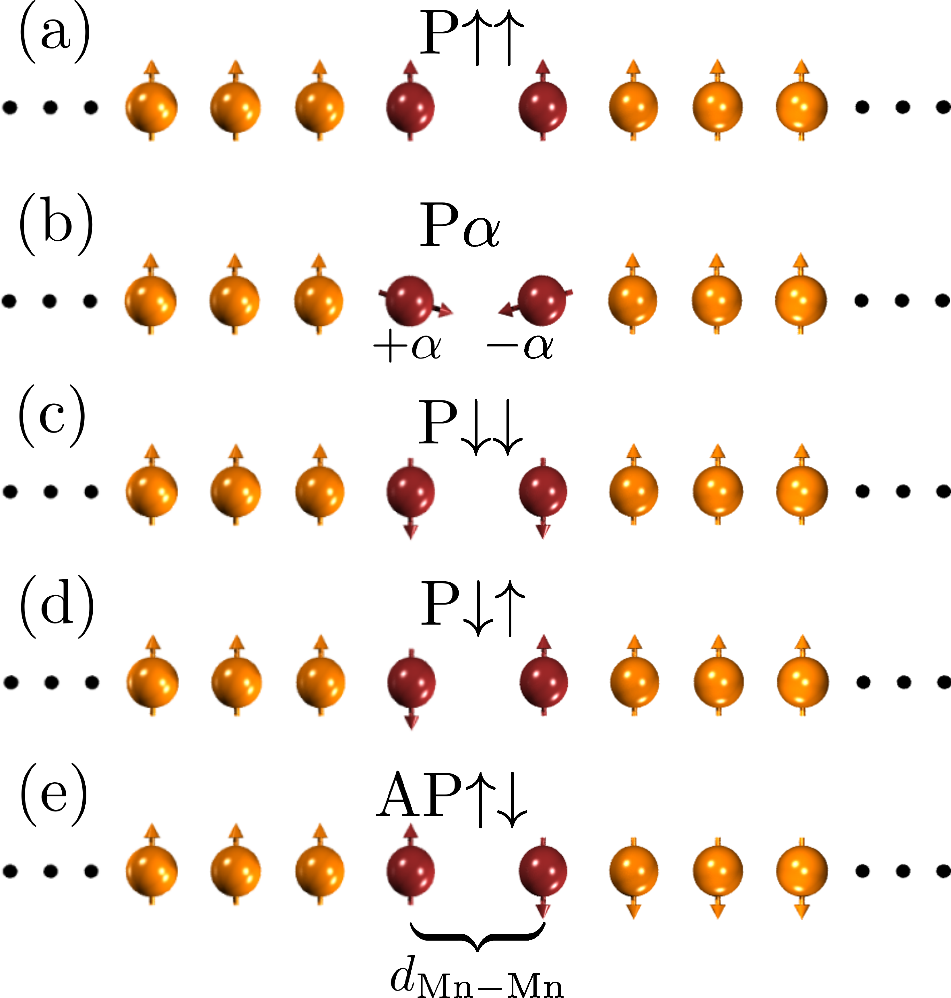
Figure 1: (color online) Calculated magnetic configurations in the $\rm{Co_{\infty}}$-$\rm{Mn}$-$\rm{Mn}$-$\rm{Co_{\infty}}$ junction. The magnetization of the left lead always points up ($\uparrow$). The magnetization of the right lead can be either parallel (P) or anti-parallel (AP) to it. The direction of the Mn spins is marked with respect to the left lead: pointing up ($\uparrow$), down ($\downarrow$), or along a direction at an angle $\alpha$ with the magnetization of the left lead. Special configurations of interest which are discussed in the text are shown: (a) P$\uparrow$$\uparrow$, (b) symmetric P$\alpha$ state with $\alpha=105^{\circ}$, P$105^{\circ}$, (c) P$\downarrow$$\downarrow$ (d) P$\downarrow$$\uparrow$ and (e) AP$\uparrow$$\downarrow$. In the text, we refer to the separation between the leads in terms of the distance between the Mn atoms, $d_{\rm{Mn-Mn}}$. Co atoms are displayed as orange spheres, Mn atoms are displayed as red spheres.

III.1 Computational details

For all collinear and non-collinear electronic structure calculations we used density functional theory within generalized gradient approximation (GGA) to the exchange-correlation potential,Zhang and Yang (1998) as implemented in the FLAPW Jülich code FLEUR.fle The wires were calculated in three-dimensional super-cells, with an interchain separation in the $x$-$y$$-$plane of 13 bohr. The super-cell setup along the chain’s axes ($z$-direction) is described in detail below. The Brillouin zone (BZ) was sampled by 12 or 24 $k$-points along the $z$-axis, depending on the size of the super-cell. All calculations were performed with an LAPW basis cut-off parameter $k_{\mathrm{max}}$ of 3.7 bohr^-1, resulting in approximately 625 LAPW basis functions per atom.

The parallel magnetic configuration (P) of $\rm{Co_{\infty}}$-$\rm{Mn}$-$\rm{Mn}$-$\rm{Co_{\infty}}$ junctions was investigated in an 8-atom super-cell along the chain direction, consisting of six Co atoms with an equilibrium interatomic distance of the Co infinite monowire of $d_{\rm{Co}}=4.15$ bohr, and two attached Mn atoms, see Fig. 1. For all considered magnetic configurations, with parallel or antiparallel alignment of the magnetization of the leads, as well as non-collinear magnetic states, irrespective of the separation between the leads, we fixed the Co-Mn distance $d_{\rm{Co-Mn}}$ to 4.48 bohr, which corresponds to the equilibrium distance between the ferromagnetic Co and Mn atoms at a very large separation between the leads. For the P$\uparrow$$\uparrow$ and P$\downarrow$$\downarrow$-states of the junction we considered the inter-Mn separation of $d_{\rm{Mn-Mn}}=5.0$, $5.5$, $7.0$, $8.5$, $10.0$, $12.5$, $15.0$, $17.5$ and $20.0$ bohr. The anti-parallel magnetic configuration (AP) of $\rm{Co_{\infty}}$-$\rm{Mn}$-$\rm{Mn}$-$\rm{Co_{\infty}}$ junctions was calculated in a 16-atom super-cell, consisting of six $\uparrow$-Co atoms and two Mn atoms on one side, and six $\downarrow$-Co atoms and two Mn atoms at another end of the junction. In this case $d_{\rm{Mn-Mn}}$ was set to 4.5, 5.0, 5.5, 7.0 and 8.5 bohr.

For the conductance calculations we applied the locking technique to a perfect monowire to describe the semi-infinite leads, as described in detail in Ref. Hardrat et al., 2012. In all cases the Wannier functions were generated on a $1\times 1\times 24$ $k$-point grid in the BZ. For the collinear cases the WFs were generated from one $4s$- and five $3d$-orbitals per atom for each spin separately, which were constructed from the radial solutions for the FLAPW potential. In non-collinear calculations the spin channels are mixed, and two $4s$- and ten $3d$-orbitals per atom were used to construct the WFs per atom. The energy bands were disentangled using the procedure described in Ref. Birkenheuer and Izotov, 2005. For the collinear calculations the lowest 58 eigenvalues per $k$-point were used to obtain 48 WFs for the 8 atom super-cell and the lowest 104 eigenvalues per $k$-point for 96 WFs for the 16 atom super-cell calculations. With non-collinearity of the magnetization included the lowest $103$ eigenvalues per $k$-point were used to obtain 96 WFs for the 8 atom unit cell. For testing purposes, for several non-collinear configurations we compared the electronic structure of the system calculated with FLEUR and with corresponding WFs, finding that a very good description of the electronic structure can be achieved with WFs within the 3rd nearest-neighbor approximation, while for WFs calculations of the transmission in the vicinity of the Fermi level already the 2nd nearest-neighbor approximation to the WFs Hamiltonian provides very reliable results.

III.2 Collinear magnetic states of the junction from tunneling to contact

We start the investigation of the $\rm{Co_{\infty}}$-$\rm{Mn}$-$\rm{Mn}$-$\rm{Co_{\infty}}$ junction with both leads positioned far away from each other. To mimic a tip-sample approach, we decrease the Mn-Mn distance $d_{\rm{Mn-Mn}}$, and calculate the energies of the collinear states P$\uparrow\uparrow$, P$\downarrow\downarrow$ and P$\downarrow\uparrow$, showing the results in Fig. 2(a). The energy difference between P$\uparrow$$\uparrow$ and P$\downarrow$$\downarrow$ states when the distance is varied in the tunneling regime from $d_{\rm{Mn-Mn}}=20$ bohr down to $10$ bohr remains relatively constant and constitutes around $27$ meV per atom, indicating weak interaction between both sides of the junction and a weak ferromagnetic coupling between the Mn atom and its nearest Co neighbor (NN Co). After a small reduction of the energy difference between the P$\uparrow$$\uparrow$ and P$\downarrow$$\downarrow$ states around $d_{\rm Mn-Mn}=8$ bohr, the ferromagnetic (FM) Mn-Co coupling becomes more stable for decreasing $d_{\rm{Mn-Mn}}$, expressed in an increasing energy difference. In the contact regime we find a slight decrease in the energy difference from 93.5 meV at $d_{\rm{Mn-Mn}}=5.0$ bohr down to $77$ meV per atom at $d_{\rm{Mn-Mn}}=4.5$ bohr. This decrease in energy can be correlated with strong changes in the Mn and NN Co spin moments, $S_{\rm{Mn}}$ and $S_{\rm{Mn}}$, respectively, upon decreasing the distance, see Fig. 2(b) and (c) (see also discussion in the next section).

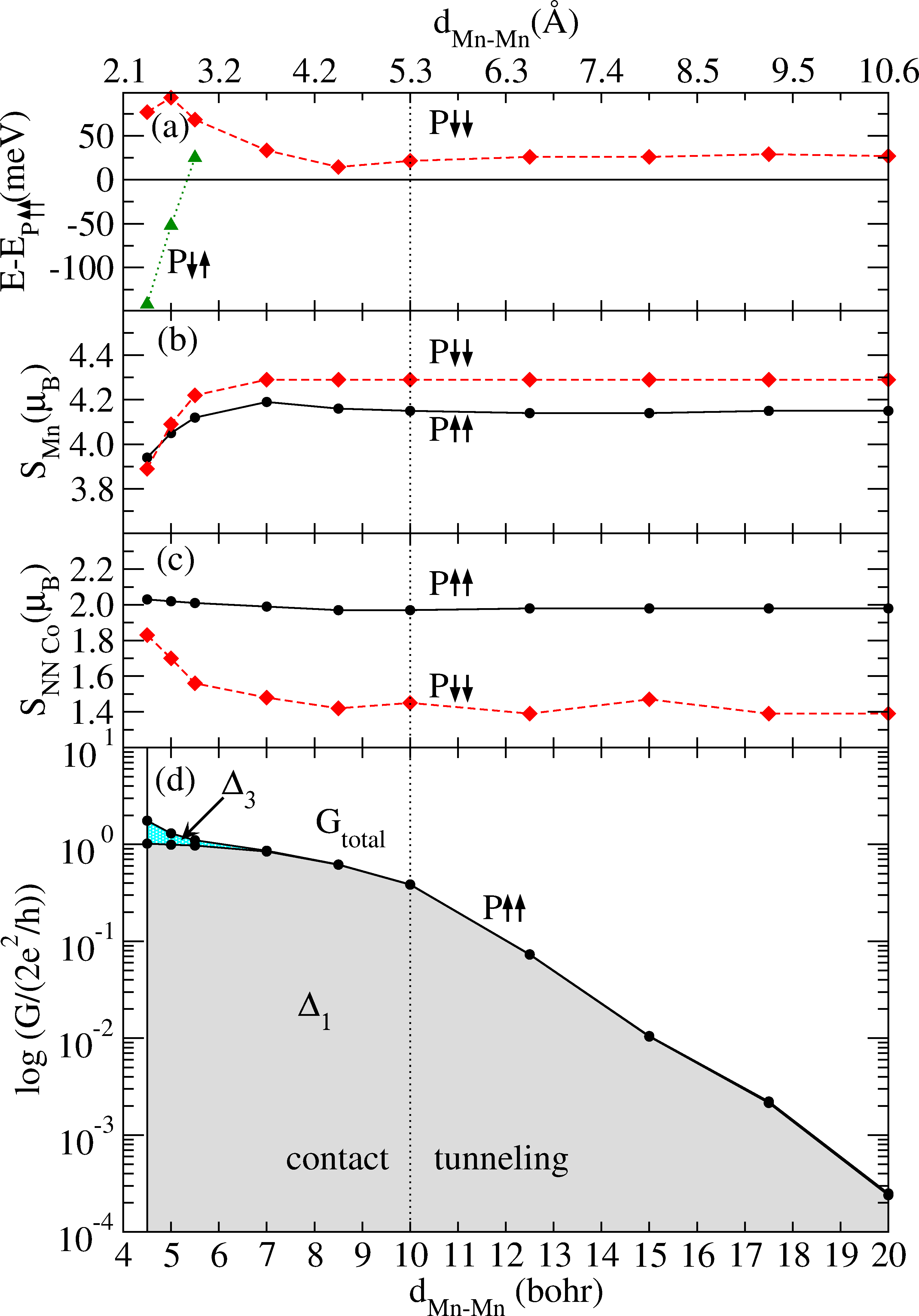
Figure 2: (color online) (a) Energy of the P$\downarrow$$\downarrow$ state (red diamonds, dashed line) and P$\downarrow$$\uparrow$ state (green triangles, dotted line) with respect to the energy of the P$\uparrow$$\uparrow$ state, as a function of the Mn-Mn interatomic distance $d_{\rm{Mn-Mn}}$. Spin moment of the Mn atoms, $S_{\rm{Mn}}$, (b), and NN Co atoms, $S_{\rm{Co}}$, (c), for P$\uparrow$$\uparrow$ (black circles, solid line) and P$\downarrow$$\downarrow$ (red diamonds, dashed line) configurations are given as a function of $d_{\rm{Mn-Mn}}$. (d) Total conductance at the Fermi level, $G_{\rm{total}}(E_{F})$ (upper line) and $\Delta_{1}$ conductance $G_{\Delta_{1}}(E_{F})$ (lower line) on a logarithmic scale for the P$\uparrow$$\uparrow$-state. Gray shaded area is associated with the $\Delta_{1}$ conductance, while cyan shaded area with the $\Delta_{3}$ conductance.

While in all cases the spin moments of the Co atoms, not neighboring the Mn atoms directly ($\approx 2.09\,\mu_{B}$) are very similar to the spin moments of the Co atom in an infinite lead ($\approx 2.07\,\mu_{B}$), the spin moments of Mn atoms and the NN Co atoms can be strongly affected by $d_{\rm{Mn-Mn}}$ at close contact and the spin configuration of the junction. Namely, for the P$\downarrow$$\downarrow$ state $S_{\rm{Mn}}$ decreases from 4.3 $\mu_{B}$ to 3.9 $\mu_{B}$, while NN $S_{\rm{Co}}$ increases from $1.4\,\mu_{B}$ to $1.8\,\mu_{B}$, as $d_{\rm{Mn-Mn}}$ is varied from 5.5 to 4.5 bohr. On the other hand, if the Mn spin moment exhibits a similar variation as a function of distance for the P$\uparrow$$\uparrow$ state, the spin moment of the NN Co atoms remains relatively constant ($\approx 2\,\mu_{B}$). This interplay between structure and magnetism already indicates that the intra-atomic as well as inter-atomic exchange, given by the Stoner parameter $I$ and the Heisenberg exchange constants $J$, respectively, may be of importance for further understanding of the magnetic properties of this system.

The change from FM coupling at larger interatomic distances to an antiferromagnetic (AFM) coupling at smaller $d_{\rm{Mn-Mn}}$ in an infinite Mn chain has been previously predicted based on DFT calculations.Mokrousov et al. (2007) In the vicinity of this crossover point the Mn spins favor non-collinear magnetic order.Schubert et al. (2011); Zelený et al. (2009); Ataca et al. (2008) To demonstrate a strong tendency of Mn spin moments to AFM coupling at smaller values of $d_{\rm{Mn-Mn}}$ we plot the energy difference between the P$\uparrow$$\uparrow$ and P$\downarrow$$\uparrow$ states in Fig. 2(a). Reversing one of the Mn spin moments in the P$\uparrow$$\uparrow$ configuration is clearly energetically more favorable than the P$\uparrow$$\uparrow$ state when the distance between the Mn atoms is below $\approx 5.2$ bohr. In this case the gain in energy due to switch of the Mn spin moment can be explained only by the strong AFM coupling of the two Mn atoms for this regime of interatomic distance, since the coupling of the Mn atom with its NN Co atom is ferromagnetic. The spin moments in the P$\downarrow$$\uparrow$ state at $d_{\rm{Mn-Mn}}=4.5$ bohr constitute $4.1\,\mu_{B}$ for Mn and $1.5\,\mu_{B}$ for its NN Co on the AFM side, and $3.7\,\mu_{B}$ for Mn and $1.9\,\mu_{B}$ for the n.n Co on the FM side. For larger $d_{\rm{Mn-Mn}}$ values the P$\uparrow$$\uparrow$ state is the lowest in energy as compared to all possible collinear states of the junction in which the magnetization direction of the left and right leads is the same, which is indicative of the FM Mn-Mn coupling for larger distances.

In Fig. 2(d) we present the results of our calculations for the evolution of the ballistic conductance of a P$\uparrow$$\uparrow$ junction when going from the tunneling to the contact regime. The main contribution to the conductance at large Mn-Mn distances is coming solely from the $\Delta_{1}$ channel, owing to the overlap between the $s$-$d_{z^{2}}$ orbitals of the neighboring Mn atoms across the barrier. Within our approach, the expected exponential behavior of the conductance at very large distances is very nicely reproduced. At a distance of $d_{\rm{Mn-Mn}}\approx 10$ bohr the conductance approaches the magnitude of the conductance quantum, reaching saturation upon further decreasing the distance. For distances in the contact regime below 7 bohr more localized $d$-orbitals of $\Delta_{3}$ symmetry start contributing to the total conductance, as can be seen in Fig. 2(d). The $\Delta_{3}$ contribution to the conductance increases with decreasing distance. As we shall see in the following the details of hybridization between the $\Delta_{3}$ orbitals are very sensitive to the magnetic state of the junction. On the other hand, in all considered cases the $d$-states of $\Delta_{4}$ symmetry do not contribute to the conductance due to an energetic mismatch between the states of this symmetry of NN Co and Mn atoms, see discussion in section III.4.

III.3 Non-collinear magnetic states of the junction in contact regime

According to the findings presented above, we expect that Mn spin moments in the contact regime will experience a frustration when the magnetizations of the leads are parallel to each other. In this case, when Mn atoms are close enough, FM coupling of Mn spins with NN Co atoms and AFM Mn-Mn coupling can possibly lead to a stable non-collinear magnetic state. In order to consider this situation, we introduce an angle $\alpha$ between the spin moments of the Mn and the NN Co atoms, rotating the first Mn spin moment by $+\alpha$ and the second one by $-\alpha$, while keeping the moments of the Co atoms fixed, see Fig. 1(b). This is what we call a symmetric P$\alpha$-state. We choose a distance of 4.5 bohr between the Mn atoms as a representative of the contact regime at which the Mn-Mn coupling is strongly antiferromagnetic.

The results of our calculations for the total energy of the P$\alpha$ state, $E_{{\rm P}\alpha}$, in relation to the energy of the P$\uparrow$$\uparrow$ state are shown in Fig. 3(a) as a function of the angle $\alpha$. From this plot we observe that the minimum of the total energy is acquired for the non-collinear P$105^{\circ}$ state, which is $137$ meV lower in energy than the corresponding collinear P$\uparrow$$\uparrow$ state. The failure of a straightforward description of the energy landscape $E_{{\rm P}\alpha}$ in terms of a simple Heisenberg model which assumes just the nearest-neighbor Co-Mn and Mn-Mn exchange coupling, given by antiferromagnetic $J_{\rm{Mn}}<0$ and ferromagnetic $J_{\rm{Co}}>0$, respectively, can be understood from noticing that the expression for the energy within this approximation, given by

$$E_{{\rm P}\alpha}(\alpha)=-\frac{1}{2}(J_{\rm{Mn}}\cos(2\alpha)+2J_{\rm{Co}}\cos(\alpha)),$$ (18)

acquires a minimum for angles $\alpha$ below $90^{\circ}$, in contradiction to our calculations.

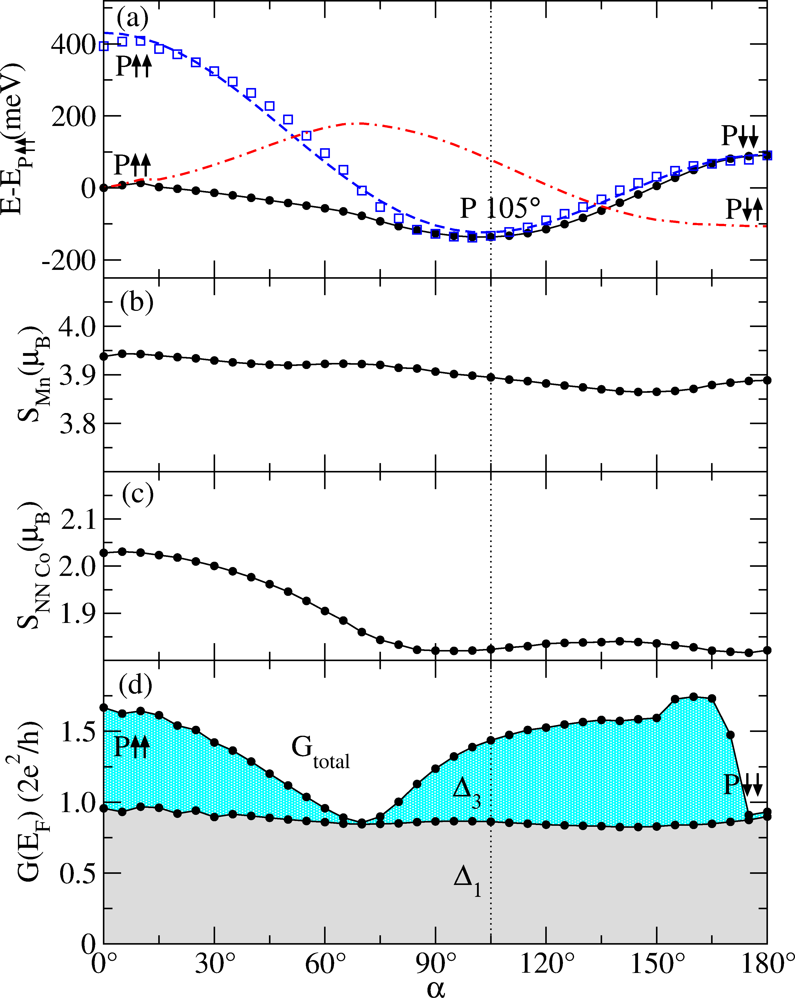
Figure 3: (color online) (a) Total energy of the P$\alpha$ state with respect to the P$\uparrow$$\uparrow$ state as a function of angle $\alpha$ (solid line, filled circles). With open black squares we show the total energy of the P$\alpha$ state from which the Stoner energy due to creation of the NN Co spin moments is subtracted. The corresponding fit of the corrected energy to the Heisenberg model is shown with a dashed blue line. With the red dotted line we show the total energy of the P$\uparrow$$\downarrow$ state with only the $\downarrow$-Mn spin rotated by an angle $\alpha$, calcualted within the Heisenberg model and incorporating also the Stoner exchange. (b) Mn spin moment as a function of angle $\alpha$. (c) NN Co spin moment as a function of angle $\alpha$. (d) Ballistic conductance at the Fermi level for the P$\alpha$ state as a function of angle $\alpha$: total conductance $G_{\rm{total}}(E_{F})$ (upper line), the $\Delta_{3}$ conductance contribution (cyan shaded area) and and $\Delta_{1}$ conductance $G_{\Delta_{1}}(E_{F})$ (lower line, gray shaded area).

The solution to this deficiency of the Heisenberg model can be given by lifting the assumption that the exchange interaction between the Mn and Co spins, given by $J_{\rm Co}$, is ferromagnetic. As we can see from Fig. 3(b) and (c), while the Mn spin moment remains relatively constant upon changing $\alpha$, $S_{\rm{Co}}$ for values of $\alpha$ below 60^∘ is by as much as $0.2\,\mu_{B}$ larger than for $\alpha>90^{\circ}$. Owing to the intra-atomic Stoner exchange, the non-collinear states with small $\alpha$ therefore acquire a negative contribution to the total energy in addition to that proportional to $J_{\rm Co}$, as compared to larger angles. If we account for the energy gain due to creation of the NN Co spin moments by a Stoner parameter of Co, $I\approx 990$ meV, Gunnarsson (1976) and subtract the energy gain $E_{\rm{Stoner}}=\frac{1}{2}IS_{\rm{Co}}^{2}$ from the calculated DFT dispersion, we arrive at the energy dispersion (squares in Fig. 3(a)), which reflects only exchange interactions between the atoms. If we fit this curve according to Eq.(18) (dashed line in Fig. 3(a)), we obtain the ”non-renormalized” Heisenberg exchange constants of $J_{\rm Co}=-170$ meV and $J_{\rm{Mn}}=-366$ meV. It becomes clear now, that, although the ”pure” exchange coupling between the Mn and Co spins is expectedly antiferromagnetic, the larger spin moment of Co in the parallel spin alignment with Mn, tips the balance in favor of ferromagnetic coupling between the spins, which can be observed for a large range of distances $d_{\rm{Mn-Mn}}$, c.f. Fig. 2(a).

In Fig. 2(a) we also observe that, judging from the energies, in the close contact regime the collinear P$\downarrow$$\uparrow$-state is competing with the non-collinear P$\alpha$-state for the global ground state of the system. Indeed, our calculations show that at the $d_{\rm{Mn-Mn}}$ of 4.5 bohr the P$\downarrow$$\uparrow$-configuration is by a tiny value of 5 meV lower in energy than the P105^∘ solution. We argue, however, that the P$\downarrow$$\uparrow$-state is not very likely to appear in experiments, given that the Co electrodes are identical. In this case, the adiabatic rise of the intrinsically asymmetric P$\downarrow$$\uparrow$-configuration via symmetric non-collinear states cannot happen, as the electrodes, initially being in the P$\uparrow$$\uparrow$-state when very far from each other, are brought together (see also discussion at the beginning of section III.5). Nevertheless, it seems plausible, that such state, if observed in experiment, is created via a rapid flip of one of the Mn atoms in the contact regime, during, e.g., a reformation of the lead geometry, or an inelastic current-induced spin-flip process. Our calculations, shown with a dotted line in Fig. 3(a), based on the Heisenberg model extended by the Stoner term of intra-atomic exchange of the Co moments, indicate, that once the system enters the P$\downarrow$$\uparrow$-state, it is effectively ”trapped” there, since the $\downarrow$-Mn is energetically quite stable versus deviations in the angle its spin makes with the rest of the spins in the system. Thus, we do not consider any non-collinear states associated with the P$\downarrow$$\uparrow$-state in the following.

III.4 Ballistic conductance of non-collinear magnetic states of the junction

In this section we perform a detailed analysis of the ballistic conductance $G(E_{F})$ of the P$\alpha$ state at fixed distance between Mn atoms of 4.5 bohr. At this distance, we calculate $G(E_{F})$ as a function of angle $\alpha$ and present the results in Fig. 3(d). In this plot we observe that the conductance exhibits a very non-trivial dependence on $\alpha$, originating mainly from the $\Delta_{3}$-orbitals ($d_{xz,yz}$), while the $\Delta_{1}$ contribution ($s-d_{z^{2}}$) to the conductance, $G_{\Delta_{1}}$, remains almost perfectly constant. Surprisingly, the $\Delta_{3}$-conductance almost vanishes for $\alpha$ of about 70^∘, away from any high-symmetry spin configuration in the junction, suggesting, that the dependence of the details of hybridization and electronic structure on the angle between the Mn spins can be rather delicate. In order to analyze this dependence in more detail, as a function of $\alpha$, we plot the energy-dependent conductance, $G(E)$, versus the local densities of states (LDOS) of Mn and NN Co atoms resolved into spin-up and spin-down contributions with respect to the global spin quantization $z$-axis, Fig. 4. Mainly we focus on the $\Delta_{3}$-contribution to the conductance and the LDOS, and only in the upper (P$\uparrow$$\uparrow$) and lower (P$\downarrow$$\downarrow$) panels of Fig. 4 we show also the total LDOS of the atoms.

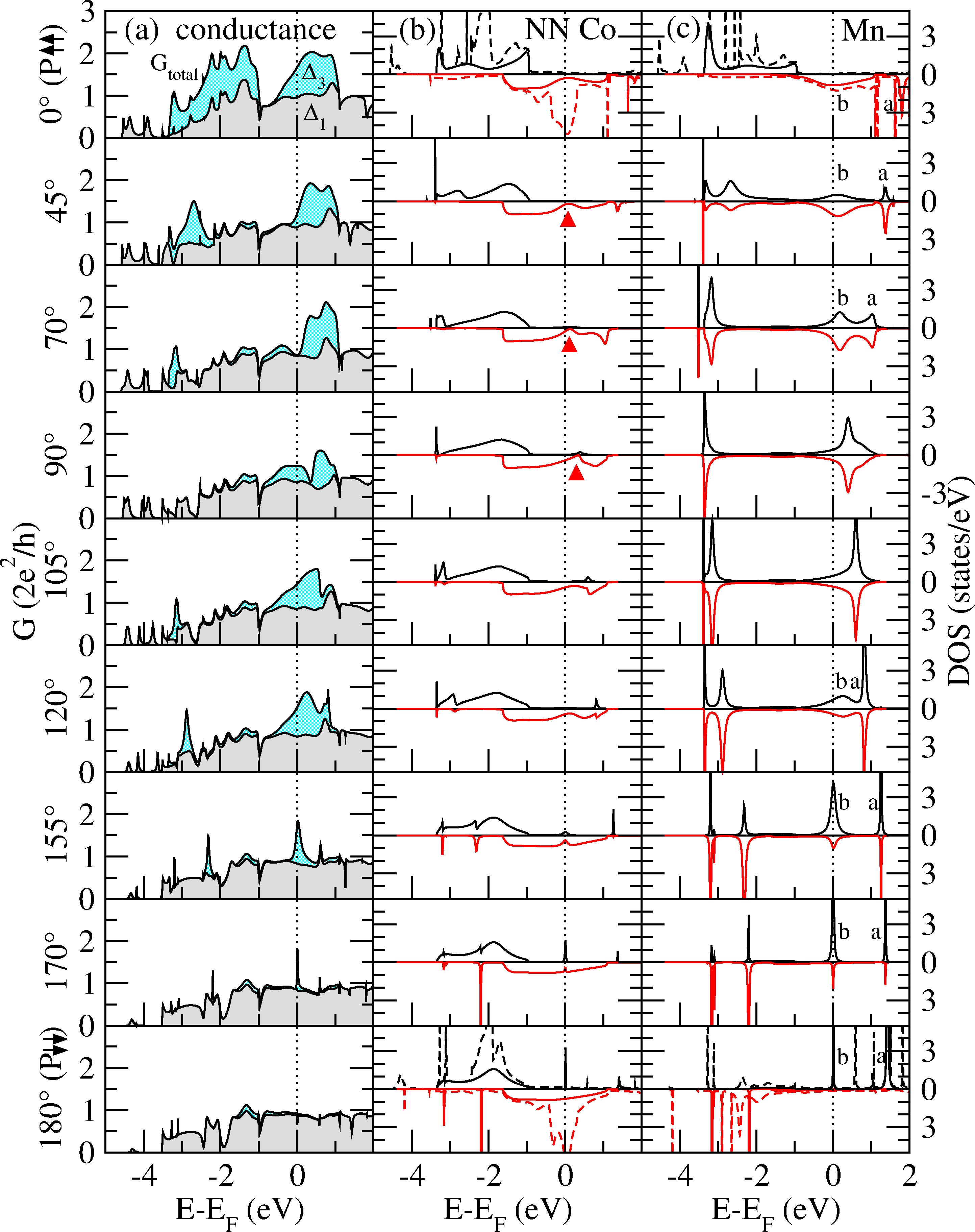
Figure 4: (color online) Transport properties and electronic structure of the P$\alpha$-state at $d_{\rm{Mn-Mn}}$ of 4.5 bohr as a function of angle $\alpha$ (indicated on the left). (a) Total conductance $G_{\rm{total}}$ (upper line) decomposed into the $\Delta_{3}$- (cyan shaded area) and $\Delta_{1}$-contributions ($G_{\Delta_{1}}$, lower line, gray shaded area). The spin-resolved local density of states (LDOS) of the NN Co atom and Mn atom are given in columns (b) and (c), respectively. For both (b) and (c) the LDOS spin-decomposition is performed with respect to the global frame, with spin-up and spin-down LDOS presented in the upper and lower parts of each plot. In both (b) and (c), the $\Delta_{3}$-contribution is indicated with solid lines, while for $\alpha=0^{\circ}$ and $\alpha=180^{\circ}$ also the total LDOS is shown with dashed lines. The red triangles in (b) follow the development of the dip in the LDOS of the NN Co atom as the angle $\alpha$ is varied. In (c), the bonding and anti-bonding unoccupied Mn states are marked with ”b” and ”a”, respectively. For details see text.

The conductance at a given energy $E$ depends on the presence of available states in the LDOS of the atoms at $E$, and on the coupling between these states across the junction $-$ both of which depend on the orientation of the spins with respect to each other. By looking at the LDOS of the atoms presented in Fig. 4 for $\alpha=0^{\circ}$ we can explain the absence of the $\Delta_{4}$ ($d_{xy,x^{2}-y^{2}}$) contribution to the conductance: the localized $\Delta_{4}$ states of the Co atoms, which can be seen as pronounced peaks in the LDOS marked with the dashed line in Fig. 4, are positioned at about $-$2 eV for spin-up channel and directly at the Fermi energy for spin-down channel, while the corresponding Mn $\Delta_{4}$ states are positioned below $-$2.5 and above $+$1 eV, prohibiting thus the hybridization between the Co and Mn orbitals of $\Delta_{4}$ symmetry across the junction. Noticeably, the LDOS of both atoms for the up-spin in a wide region of energies around $E_{F}$ is absent, leading to a negligible $\uparrow$-conductance. Here, it is important to remark, that the LDOS of the NN Co atoms around the Fermi energy overall resembles quite well the LDOS of a Co atom in a Co monowire, see e.g. Fig. 13(a) in Ref. Hardrat et al., 2012, or even of a Co atom deposited on a noble-metal surfaces, see e.g. Ref. Nonas et al., 2001. This means that our results should be rather stable with respect to the geometry of the Co leads, manifesting that the main influence on the $\Delta_{3}$ conductance at $E_{F}$ would come from the hybridization of the Mn and NN Co states.

Turning now to the comparatively delocalized $\Delta_{3}$-states (solid line) on both Co and Mn atoms, we observe for P$\uparrow\uparrow$ (upper panels of Fig. 4) that they hybridize directly at the Fermi energy, which leads to a significant $\Delta_{3}$ contribution to the conductance. Specifically, while the $\Delta_{3}^{\downarrow}$ subband of Co spreads from $-$1.8 to $+$1 eV, the $\Delta_{3}$-down states of Mn atoms are distinctly split into wide bonding (”b”) states at the Fermi energy and narrow anti-bonding (”a”) states at $+$1.8 eV. Very importantly for the transport properties of the system, the hybridization of the $\Delta_{3}^{\downarrow}$ band of Co with the $\Delta_{3}^{\downarrow}$ states of Mn is non-trivial. (i) The $\Delta_{3}^{\downarrow}$ states of Co exhibit a dip at the position of the maximal density of bonding states of Mn due to the fact that these Mn states are localized mainly in between the Mn atoms prohibiting strong overlap with the Co states. (ii) The upper, antibonding, part of the Co $\Delta_{3}^{\downarrow}$ band hybridizes stronger with the bonding states of Mn, since the antibonding states of Co atoms have a larger overlap with the Mn orbitals, which results in a larger $\Delta_{3}$-conductance above $E_{F}$. (iii) Analogously, for energies below $E_{F}$ the conductance is suppressed, since the bonding-like $\Delta_{3}^{\downarrow}$ Co states have smaller overlap with the Mn bonding states.

Let us now follow the evolution of the electronic structure upon increasing the angle between the Mn spins. Two trends in the LDOS can be clearly observed in Fig. 4. Firstly, with increasing $\alpha$ the splitting between the bonding and antibonding Mn states decreases owing to the mixed spin character of the states. At the angle of 90^∘, when Mn spins are anti-parallel to each other, both types of states transform into degenerate $\Delta_{3}$-orbitals of the ”isolated” Mn atoms, since the hybridization between the Mn states of the same spin is almost absent due to large exchange splitting. On the other hand, the dip in the $\downarrow$-LDOS of the NN Co atoms follows the position of the bonding state of the Mn dimer, moving from the Fermi energy at $\alpha=0^{\circ}$ to $+$0.2 eV for $\alpha=90^{\circ}$ (indicated by filled triangles in Fig. 4). Overall, such redistribution of the LDOS of the atoms combined with the effect of decreasing LDOS of Mn atoms for spin-down channel at the Fermi energy when the angle $\alpha$ is varied, results first in a decrease of the conductance at $E_{F}$ for $\alpha\approx 70^{\circ}$, followed by a consequent increase with increasing angle.

When the angle $\alpha$ increases further beyond 90^∘, the bonding and anti-bonding Mn states eventually acquire their initial splitting at $\alpha=180^{\circ}$ (P$\downarrow$$\downarrow$-state), when the Mn spins are collinear again. Simultaneously, with increasing angle, we observe that the Mn states around the Fermi energy become sharper, since the hybridization with the Co leads decreases as the Mn states become predominantly spin-up in character. Interestingly, while for $90^{\circ}<\alpha<120^{\circ}$ a large value of the $\Delta_{3}$-conductance is due to a significant amount of delocalized Co and bonding Mn states at the Fermi energy in the spin-down channel, for larger angles the value of $G_{\Delta_{3}}(E_{F})$ is due to a sharp resonant Co state in the spin-up channel at the Fermi energy, coupled to a bonding Mn state at $E_{F}$. When further increasing $\alpha$ above 170^∘, this resonance becomes more localized and decoupled from the states in the leads, while the Mn LDOS at the $E_{F}$ in the minority spin-channel vanishes, causing a sharp drop in the $\Delta_{3}$-conductance. By looking at the total LDOS of the NN Co atom in the P$\downarrow$$\downarrow$-state we observe that it remains basically unaffected, as compared to the P$\uparrow$$\uparrow$-configuration, while the Mn states become pronouncedly decoupled from the states of the NN Co owing to the energetical mismatch for both spin channels.

III.5 Fingerprints of non-collinear magnetic states of the junction in ballistic conductance experiments

Finally, we investigate the evolution of the conductance and the magnetoresistance of different magnetic states of the junction within the contact regime mimicking a typical STM or break junction experiment. Here, we are partly motivated by the fact that a non-trivial behavior of magnetoresistance when going from tunelling to contact has been recently observed in STM experiments, see e.g. Ref. Ziegler et al., 2011. At a very large separation between the leads (or, the tip and the sample in the STM language), owing to the FM coupling of the Mn atom to the Co chain, one can imagine only two possible magnetic configurations $-$ P$\uparrow$$\uparrow$ and AP$\uparrow$$\downarrow$. The conductance of these two magnetic states in the tunneling regime, arising mainly from the $s$-orbitals, is orders of magnitude smaller than in the contact regime, for which the dependence of $G(E_{F})$ on the distance can be non-trivial due to the large contribution of the $d$-states.

In the case of the AP$\uparrow$$\downarrow$ configuration, the starting collinear arrangement of the spins will survive over the whole range of the separation between the leads, since in the contact regime, when the Mn atoms are close to each other, both exchange preferences of the Mn spins, that is, FM coupling to the NN Co spins and AFM coupling among each other, are fulfilled. Small possible deviations from the collinear arrangement of the Mn spins, which can affect the details of the distribution of the $\Delta_{3}$-states and their coupling to the leads, would not manifest in a conductance measurement, owing to the antiparallel magnetizations of the leads, and corresponding complete dominance of the $\Delta_{1}$ channel for conductance at $E_{F}$ in this case, Fig. 5. As we can see from this figure, $G(E_{F})$ lies in between 0.5 and 1.0$\,G_{0}$, when the distance between the Mn atoms is varied from 8.5 to 4.5 bohr. This is very similar to the behavior of the conductance at the Fermi energy of pure AP Co leads without Mn atoms, see e.g. Fig. 11(b) of Ref. Hardrat et al., 2012.

Owing to the magnetic frustration of the Mn spins of the junction in the contact regime, for the P$\uparrow$$\uparrow$ initial configuration, we consider the P$\alpha$ and P$\downarrow$$\uparrow$ states in addition to the P$\uparrow$$\uparrow$ state when the Mn-Mn distance is relatively small. Here, as we have seen in the preceding section, the conductance at the Fermi energy can be very strongly influenced by the details of hybridization between the $\Delta_{3}$-orbitals. On the other hand, since very often transport measurements serve as the only experimental insight into the magnetic structure of a system, it is very important to coin each of the possible magnetic states with a unique fingerprint which can be related to the experimental data. Below, we suggest that indeed three distinct spin states in a $\rm{Co_{\infty}}$-$\rm{Mn}$-$\rm{Mn}$-$\rm{Co_{\infty}}$  junction $-$ which can occur in an experiment due to various reasons such as structural details, temperature fluctuations, external magnetic field, etc. $-$ lead to different transport signatures.

As already shown in Fig. 2(d), the conductance of the collinear P$\uparrow$$\uparrow$ state rapidly rises towards a value of 1.8$\,G_{0}$ as the distance between the leads is decreased. Compared to other possible magnetic configurations of the junction, $G_{{\rm P}\uparrow\uparrow}(E_{F})$ is significantly larger in value, see Fig. 5, because of the alignment of the minority spin $s$- and $d$-states of the Co electrodes and the Mn atoms at the Fermi energy, which ideally favors perfect transmission. In contrast, the conductance of the collinear P$\downarrow$$\uparrow$-state is significantly suppressed, reaching only 1.0$\,G_{0}$ at the separation of 4.5 bohr, due to the large exchange splitting of the $\Delta_{3}$ states of the Mn atoms with antiparallel spin moments which hinders the $\Delta_{3}$ conductance. The conductance of the non-collinear ground-state P$\alpha$-state lies in between the values for both limiting collinear configurations. In the close contact regime, at $d_{\rm{Mn-Mn}}$ of 4.5 bohr, the conductance of the P$\alpha$-state of 1.4$\,G_{0}$ is exactly in between the values of $G_{{\rm P}\uparrow\uparrow}(E_{F})$ and $G_{{\rm P}\downarrow\uparrow}(E_{F})$. Clearly, the difference of 0.4$\,G_{0}$, stemming from the variation in the $\Delta_{3}$-conductance with the spin state, can be easily detected in experiment, allowing for a way to distinguish between different possible magnetic configurations. At the distance of 5.0 bohr the ground state among the P$\alpha$ states is the P90^∘ state, while at larger distances above 5.5 bohr the system converges to a collinear configuration. The angle $\alpha$ in the lowest in energy P$\alpha$ state decreases smoothly with increasing the separation, and we speculate, that owing to the non-monotonous behavior of the conductance as a function of $\alpha$, seen in Fig. 3(d), the conductance as a function of $d_{\rm Mn-Mn}$, can exhibit several features similar to that at $d_{\rm Mn-Mn}$ of 5.0 bohr, although we did not perform the calculations to support this statement owing to the required computational effort.

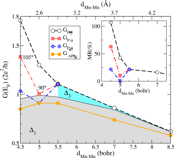
Figure 5: (color online) Conductance at the Fermi energy of various possible magnetic states of the $\rm{Co_{\infty}}$-$\rm{Mn}$-$\rm{Mn}$-$\rm{Co_{\infty}}$  junction as a function of the distance between the Mn atoms. Following magnetic states are considered: AP$\downarrow$$\uparrow$ (filled circles, solid line), P$\uparrow$$\uparrow$ (open circles, dashed line), P$\downarrow$$\uparrow$ (diamonds, dash-dash-dotted line), and P$\alpha$ (squares, dot-dashed line). The $\Delta_{1}$ contribution for the P$\uparrow$$\uparrow$-state is shown with a thin solid line and grey shaded area, while the $\Delta_{3}$ part is shaded in cyan. For the P$\alpha$ states the state which is lowest in energy among all possible angles $\alpha$ at a fixed distance is considered. In the inset the values of the magnetoresistance for different P-states are shown.

According to recent experiments,Ziegler et al. (2011) the conductance of the junction with the parallel (P) and antiparallel (AP) orientation of the lead’s magnetization can be related to each other via measuring the magnetoresistance (MR). From the values presented in Fig. 5 we calculate the MR of the junction, defined as:

$$\mathrm{MR}=\frac{G_{\mathrm{P}}(E_{F})-G_{\mathrm{AP}}(E_{F})}{G_{\mathrm{AP}}(E_{F})}\times 100\%,$$ (19)

and present the MR as a function of separation between the electrodes in the inset of Fig. 5, where we choose $G_{{\rm AP}\downarrow\uparrow}$ for $G_{\mathrm{AP}}(E_{F})$, and values of $G_{{\rm P}\uparrow\uparrow}(E_{F})$, $G_{{\rm P}\downarrow\uparrow}(E_{F})$ and $G_{{\rm P}\alpha}(E_{F})$ for $G_{\mathrm{P}}(E_{F})$. The overall smaller AP$\downarrow$$\uparrow$ conductance as compared the P-configurations results in positive magnetoresistance values. The MR curves as a function of the distance generally resemble those of the conductance, with the values of the MR of 22, 62 and 105% at the distance of 4.5 bohr for the P$\downarrow$$\uparrow$, P$\alpha$ and P$\uparrow$$\uparrow$-states, respectively. Much more pronounced in the MR is the feature characteristic to the P$\downarrow$$\uparrow$ and P$\alpha$-configurations $-$ a dip around the distance of 5.0 bohr, also present in the conductance curves. As can be seen from Fig. 5, at this distance, the MR almost completely vanishes when the Mn spins exhibit a different from FM configuration. Overall, we conclude, that the pronounced difference in the shape and magnitude of the MR curves can be also used in experiments to shed light onto the complex magnetism in this type of systems.

IV Summary

In this work we presented the realization of a first principles scheme for calculating the ballistic transport properties of magnetically complex one-dimensional systems employing the technique of non-collinear Wannier functions. We use the FLAPW method in order to calculate the electronic structure of the system with high accuracy and use the Wannier functions to transfer it to our transport calculations performed within the Landauer approach. As spin-orbit interaction can be naturally included into the consideration within this technique, c.f. Ref. Hardrat et al., 2012, the method introduced here can be used to explore the rich field of transport phenomena in systems such as nano- or atomic-sized contacts, break junctions, or STM experiments for which both effects, spin-orbit coupling and frustrated exchange interactions, can be prominent.

As a first application of our approach, we consider the ballistic transport properties of a single-atom junction formed by two semi-infinite Co electrodes with a single apex Mn atom. We study the conductance as a function of the separation between the two Mn atoms from the tunneling to the contact regime taking into account the complex magnetic interaction in the junction. As we demonstrate, even such a simple setup allows to draw some general conclusions concerning the interplay of structure and magnetism for the transport through such atomic-sized contacts which are in the focus of today’s research. We analyze the ballistic conductance of the junction with lead magnetizations in parallel and antiparallel alignment. We consider separately the tunneling (separation larger than about 5 Å) and contact (below 5 Å) regimes of the junction, and we demonstrate that in the tunneling regime the conductance $G$ is solely coming from the overlap between the $\Delta_{1}$ ($s$-$d_{z^{2}}$-orbitals) of the contacts. In this case the Mn spins prefer to order ferromagnetically with respect to the magnetization of the leads. On the other hand, upon reaching the close contact regime (below 3.5 Å), when the magnitude of the conductance reaches 1$\,G_{0}$, the hybridization between the $\Delta_{3}$ ($d_{xz},d_{yz}$-orbitals) states of the junction starts to provide a sizable contribution to $G$.

In the close contact regime, when the hybridization between the Mn atoms is significant, Mn spins experience a frustration due to the FM coupling with the leads and an AFM Mn-Mn coupling. The competition between the two gives rise to a stable non-collinear solution which can be characterized by a tilting angle of the spins, $\alpha$. General for this type of junction is the sensitivity of the $d$-orbital conductance on the angle $\alpha$, which is due to a delicate interplay between the hybridization details of the Mn and Co states at the Fermi energy, as well as spin-asymmetry in their distribution. This gives rise to a non-trivial $\alpha$-dependence of the conductance of the $d$-states. We show that the complicated $\Delta_{3}$-channel conductance arising on the background of almost constant $\Delta_{1}$ contribution can be used in order to distinguish between different magnetic states of the contact via either a direct conductance measurement, or via measuring the magnetoresistance, which, according to our calculations, can vary in the contact regime between 20 and 100%, depending on the spin arrangement.

Finally, we would like to comment on our approximation for the geometry of the junction we have assumed in this work. Albeit being very simple, it allows to capture the key features which govern the transport properties of the system, while keeping the computational burden reasonable. Namely, within this geometry: (i) the transition from tunneling to contact can be naturally studied; (ii) the magnetic frustration of the spins in the junction, and (iii) the delicate details of the hybridization of the adatom with the lead reservoirs are taken into account; (iv) the sensitive dependence of the spin moments on the magnetic configuration in the nano-contact is included into our considerations. Of course, in order to achieve a quantitative agreement of the calculated values to the experimentally measured ones in this type of junction beyond the major trends, all details of the structure and structural reformation upon approaching should be ideally accounted for. Such a challenging study lies, however, outside of the scope of the current work, and we leave it for future studies.

V Acknowledgment

We acknowledge helpful discussions with Stefan Blügel. Funding by the DFG within the SFB677 is gratefully acknowledged. S.H. thanks the DFG for financial support under HE3292/8-1. Y.M. and F.F. gratefully acknowledge the Jülich Supercomputing Centre for computing time and funding under the HGF-YIG Programme VH-NG-513.

References

- Yanson et al. (1998) A. I. Yanson, G. R. Bollinger, H. E. van den Brom, N. Agrait, and J. M. van Ruitenbeek, Nature 395, 783 (1998).
- Thiess et al. (2008) A. Thiess, Y. Mokrousov, S. Blügel, and S. Heinze, Nano Letters 8, 2144 (2008).
- Néel et al. (2009) N. Néel, J. Kröger, and R. Berndt, Phys. Rev. Lett. 102, 086805 (2009).
- Kröger et al. (2008) J. Kröger, N. Néel, and L. Limot, J. Phys. Cond. Mat. 20, 223001 (2008).
- Tao et al. (2010) K. Tao, I. Rungger, S. Sanvito, and V. S. Stepanyuk, Phys. Rev. B 82, 085412 (2010).
- Chopra et al. (2005) H. D. Chopra, M. R. Sullivan, J. N. Armstrong, and S. Z. Hua, Nature Materials 4, 832 (2005).
- Calvo et al. (2009a) M. Calvo, J. Fernández-Rossier, J. Palacios, D. Jacob, D. Natelson, and C. Untiedt, Nature 458, 1150 (2009a).
- Ziegler et al. (2011) M. Ziegler, N. Néel, C. Lazo, P. Ferriani, S. Heinze, J. Kröger, and R. Berndt, New J. Phys. 17, 085011 (2011).
- Schmaus et al. (2011) S. Schmaus, A. Bagrets, Y. Nahas, T. K. Yamada, A. Bork, M. Bowen, E. Beaurepaire, F. Evers, and W. Wulfhekel, Nature Nanotechnology 6, 185 (2011).
- Calvo et al. (2009b) M. R. Calvo, J. Fernández-Rossier, J. J. Palacios, D. Jacob, D. Natelson, and C. Untiedt, Nature 458, 1150 (2009b).
- Delin and Tosatti (2003) A. Delin and E. Tosatti, Phys. Rev. B 68, 144434 (2003).
- Smogunov et al. (2008a) A. Smogunov, A. Dal Corso, A. Delin, R. Weht, and E. Tosatti, Nature Nanotechnology 3, 22 (2008a).
- Delin et al. (2004) A. Delin, E. Tosatti, and R. Weht, Phys. Rev. Lett. 92, 057201 (2004).
- Thiess et al. (2009) A. Thiess, Y. Mokrousov, S. Heinze, and S. Blügel, Phys. Rev. Lett. 103, 217201 (2009).
- Thiess et al. (2010) A. Thiess, Y. Mokrousov, and S. Heinze, Phys. Rev. B 81, 054433 (2010).
- Hardrat et al. (2012) B. Hardrat, N.-P. Wang, F. Freimuth, Y. Mokrousov, and S. Heinze, Phys. Rev. B 85, 245412 (2012).
- Smogunov et al. (2004) A. Smogunov, A. Dal Corso, and E. Tosatti, Phys. Rev. B 70, 045417 (2004).
- Smogunov et al. (2006) A. Smogunov, A. Dal Corso, and E. Tosatti, Phys. Rev. B 73, 075418 (2006).
- Bagrets et al. (2004) A. Bagrets, N. Papanikolaou, and I. Mertig, Phys. Rev. B 70, 064410 (2004).
- Bagrets et al. (2007) A. Bagrets, N. Papanikolaou, and I. Mertig, Phys. Rev. B 75, 235448 (2007).
- Polok et al. (2011) M. Polok, D. V. Fedorov, A. Bagrets, P. Zahn, and I. Mertig, Phys. Rev. B 83, 245426 (2011).
- Burton et al. (2006) J. D. Burton, R. F. Sabirianov, S. S. Jaswal, E. Y. Tsymbal, and O. N. Mryasov, Phys. Rev. Lett. 97, 077204 (2006).
- Czerner et al. (2008) M. Czerner, B. Y. Yavorsky, and I. Mertig, Phys. Rev. B 77, 104411 (2008).
- Czerner et al. (2010) M. Czerner, B. Y. Yavorsky, and I. Mertig, Phys. Status Solidi B 247, 2594 (2010).
- Smogunov et al. (2008b) A. Smogunov, A. Dal Corso, and E. Tosatti, Phys. Rev. B 78, 014423 (2008b).
- Velev et al. (2005) J. Velev, R. F. Sabirianov, S. S. Jaswal, and E. Y. Tsymbal, Phys. Rev. Lett. 94, 127203 (2005).
- Bolotin et al. (2006) K. I. Bolotin, F. Kuemmeth, and D. C. Ralph, Phys. Rev. Lett. 97, 127202 (2006).
- Burton et al. (2007) J. D. Burton, R. F. Sabirianov, J. P. Velev, O. N. Mryasov, and E. Y. Tsymbal, Phys. Rev. B 76, 144430 (2007).
- Tao et al. (2009) K. Tao, V. S. Stepanyuk, W. Hergert, I. Rungger, S. Sanvito, and P. Bruno, Phys. Rev. Lett. 103, 057202 (2009).
- Serrate et al. (2010) D. Serrate, P. Ferriani, Y. Yoshida, S.-W. Hla, M. Menzel, K. von Bergmann, S. Heinze, A. Kubetzka, and R. Wiesendanger, Nature Nanotechnology 5, 350 (2010).
- Menzel et al. (2012) M. Menzel, Y. Mokrousov, R. Wieser, J. E. Bickel, E. Vedmedenko, S. Blügel, S. Heinze, K. von Bergmann, A. Kubetzka, and R. Wiesendanger, Phys. Rev. Lett. 108, 197204 (2012).
- Hohenberg and Kohn (1964) P. Hohenberg and W. Kohn, Phys. Rev. 136, B864 (1964).
- Kurz et al. (2004) P. Kurz, F. Förster, L. Nordström, G. Bihlmayer, and S. Blügel, Phys. Rev. B 69, 024415 (2004).
- Wannier (1937) G. H. Wannier, Phys. Rev. 52, 191 (1937).
- Marzari and Vanderbilt (1997) N. Marzari and D. Vanderbilt, Phys. Rev. B 56, 12847 (1997).
- Freimuth et al. (2008) F. Freimuth, Y. Mokrousov, D. Wortmann, S. Heinze, and S. Blügel, Phys. Rev. B 78, 035120 (2008).
- (37) URL www.flapw.de.
- Krakauer et al. (1979) H. Krakauer, M. Posternak, and A. J. Freeman, Phys. Rev. B 19, 1706 (1979).
- Mokrousov et al. (2005) Y. Mokrousov, G. Bihlmayer, and S. Blügel, Phys. Rev. B 72, 045402 (2005).
- Kizuka (2008) T. Kizuka, Phys. Rev. B 77, 155401 (2008).
- Zhang and Yang (1998) Y. Zhang and W. Yang, Phys. Rev. Lett. 80, 890 (1998).
- Birkenheuer and Izotov (2005) U. Birkenheuer and D. Izotov, Phys. Rev. B 71, 125116 (2005).
- Mokrousov et al. (2007) Y. Mokrousov, G. Bihlmayer, S. Blügel, and S. Heinze, Phys. Rev. B 75, 104413 (2007).
- Schubert et al. (2011) F. Schubert, Y. Mokrousov, P. Ferriani, and S. Heinze, Phys. Rev. B 83, 165442 (2011).
- Zelený et al. (2009) M. Zelený, M. Šob, and J. Hafner, Phys. Rev. B 80, 144414 (2009).
- Ataca et al. (2008) C. Ataca, S. Cahangirov, E. Durgun, Y.-R. Jang, and S. Ciraci, Phys. Rev. B 77, 214413 (2008).
- Gunnarsson (1976) O. Gunnarsson, Journal of Physics F: Metal Physics 6, 587 (1976).
- Nonas et al. (2001) B. Nonas, I. Cabria, R. Zeller, P. H. Dederichs, T. Huhne, and H. Ebert, Phys. Rev. Lett. 86, 2146 (2001).