Excited states in Richardson pairing model: ’probabilistic’ approach

Abstract

Richardson equations can be mapped on the classical electrostatic problem in two dimensions. We have recently suggested a new analytical approach to these equations in the thermodynamical limit, which is based on the ’probability’ of the system of charges to be in a given configuration at the effective temperature equal to the interaction constant. In the present paper, we apply this approach to excited states of the Richardson pairing model. We focus on the equally-spaced situation and address arbitrary fillings of the energy layer, where interaction acts. The ’partition function’ for the classical problem on the plane, which is given by Selberg-type integral, is evaluated exactly. Three regimes for the energy gap are identified, which can be treated as the dilute regime of pairs, BCS regime, and dilute regime of holes.

010, 062, 368

1 Introduction

Bardeen-Cooper-Schrieffer (BCS) theory plays a very important role in the microscopic description of superconductivity.[1, 2, 3]  As shown by Richardson,[4]  BCS Hamiltonian turns out to be exactly solvable. By staying in the canonical ensemble, Richardson managed to find a many-body wave function, which depends on the set of energy-like quantities (rapidities) and provides an exact solution of the Schrödinger equation. The number of rapidities is equal to the number of Cooper pairs in the system, while the Hamiltonian eigenvalue is given by their sum. Rapidities satisfy the system of nonlinear algebraic equations, now called Richardson equations. The resolution of these equations is a formidable task. More recently, it was shown that Richardson equations can be derived from the algebraic Bethe-ansatz approach.[5]  They are also closely related to the well-known Gaudin model[6] and Chern-Simons theories.[7]  Richardson equations are now widely used to study numerically superconducting state in nanometer-scale systems.[8, 9]  In particular, powerful tools of the quantum inverse scattering method were used to compute correlation functions[10] in such systems.

It is quite remarkable that Richardson equations can be mapped onto the classical electrostatic problem in the plane.[6, 11]  Namely, energy-like quantities may be treated as coordinates of interacting charged particles, which are placed into the external electric field. Equilibrium positions of these charges are then equivalent to solutions of Richardson equations. The origin of this highly remarkable example of quantum-to-classical correspondence is unclear.

We recently pushed further[12] the analogy with the classical electrostatic problem by introducing the occupation ’probability’ for the system of charges at the effective ’temperature’ given by the interaction amplitude, which goes to zero in the thermodynamical limit. This leads to the new approach to treat analytically Richardson equations. Namely, one can reconstruct an information on the location of the center of masses for the free charges by using an integration instead of a straightforward resolving the equations. This is done by constructing the ’partition function’, given by the Selberg-type integral, so that the energy of the initial quantum problem is determined by the logarithmic derivative of this classical quantity with respect to the inverse temperature. Note that Selberg integrals are familiar in conformal field theory and in random-matrix models. This fact suggests an interesting link with these subjects.

In the present paper, we extend the ’probabilistic’ approach to excited states of Richardson pairing model, which amounts manipulating more sophisticated and general Selberg-type integrals. The ’partition function’ for the deterministic problem is found analytically by converting such an integral into a coupled binomial sum, evaluated using combinatorial properties of Vandermonde matrix. We then calculate energy difference (gap) between excited and ground states, which is a more subtle quantity than the ground state energy itself. At the same time, this quantity is much more important, since it is not possible to test ground state energy experimentally in contrast to the gap. We focus on the equally-spaced model and treat arbitrary fillings of the energy interval, where attraction between up and down spin electrons acts. This can be seen[13] as a toy model for the density-induced crossover between individual fermionic molecules and a dense regime of BCS pairs.[14, 15]  We identify three different regimes for the energy of the excited state. The first one corresponds to low densities of pairs; the excitation energy in this case is controlled by the single-pair binding energy. The second regime corresponds to the dense regime of pairs. It is described by the gap of BCS type, which has a cooperative origin. The third regime is a ’superdense’ regime of pairs or a dilute regime of holes, which is again controlled by the single-pair binding energy.

The paper is organized as follows. In §2, we briefly formulate the problem and outline basic ingredients of our method. In §3, we calculate the ’partition function’. In §4, we discuss our results and we conclude in §5.

2 General formulation

We consider electrons with up and down spins, which interact through the BCS potential. The Hamiltonian is given by

$$H=\sum_{\mathbf{k}}\varepsilon_{\mathbf{k}}\left(a_{\mathbf{k}\uparrow}^{\dagger}a_{\mathbf{k}\uparrow}+a_{\mathbf{k}\downarrow}^{\dagger}a_{\mathbf{k}\downarrow}\right)-V\sum_{\mathbf{k},\mathbf{k}^{\prime}}a_{\mathbf{k}^{\prime}\uparrow}^{\dagger}a_{-\mathbf{k}^{\prime}\downarrow}^{\dagger}a_{-\mathbf{k}\downarrow}a_{\mathbf{k}\uparrow}.$$ (1)

We stay in the canonical ensemble, i.e., with the number of electrons fixed. In this case, the eigenvalue of Hamiltonian, given by equation (1), can be represented as a sum of $N$ energy-like quantities $R_{j}$, which satisfy the system of $N$ coupled Richardson equations

$$1=\sum_{\mathbf{k}}\frac{V}{2\varepsilon_{\mathbf{k}}-R_{j}}+\sum_{l,l\neq j}\frac{2V}{R_{j}-R_{l}}.$$ (2)

It is assumed that the attraction between spin up and spin down electrons acts only for the free electron states having kinetic energies confined between $\varepsilon_{F_{0}}$ and $\varepsilon_{F_{0}}+\Omega$; the same therefore applies to the sums in the right-hand side (RHS) of equation (2). The first quantity $\varepsilon_{F_{0}}$, within the traditional BCS framework, can be associated with the Fermi energy of the filled Fermi sea of noninteracting electrons, while $\Omega/2$ is the Debye frequency. We then also assume that all the energies of free electron states are different and they are distributed equidistantly within this potential layer. Such a situation is usually refereed to as the equally-spaced model. It can be understood in terms of a constant density of energy states. The distance between two nearest levels is given by $1/\rho$, where $\rho$ is the density of energy states. This means that we consider a situation with the discrete energy spectrum, but the distance between nearest energy levels for noninteracting electrons goes to zero in the thermodynamical limit, so that it becomes quasi-continuous. Thus, there are in total $N_{\Omega}=\rho\Omega$ available energy states of each spin direction in the potential layer. We fill this potential layer by $N$ pairs. In the usual BCS configuration, $N=N_{\Omega}/2$ (half-filling), while we address the arbitrary filling corresponding to macroscopic $N$ (finite density of pairs). In other words, we consider a thermodynamical limit, for which the dimensionless interaction constant $v\equiv\rho V$ stays independent on $N$, as well as the filling $N/N_{\Omega}$, whereas $\rho\sim N$. Now we take the limit $N\rightarrow\infty$. Changing the filling should be considered as a toy model for the density-induced crossover from the dilute regime of pairs, when the filling is small, to the dense regime, when the filling is increased.[16, 13]  This crossover attracts a lot of attention in the field of ultracold gases. In addition, it can be relevant for high-$T_{c}$ cuprates.[17, 18]  Such a toy model also helps to establish a link between the single-pair problem solved by Cooper and many-pair BCS condensate. It was argued[16] that this model can be directly applicable to some semiconductors. Moreover, it has obvious similarities with the well-known Eagles model[15], which however does not assume constant density of states.

There are two types of lowest excited states in Richardson approach to the pairing problem. Excitations of the first kind correspond to one of the rapidities having zero imaginary part and located between two free electron levels, i.e., in a quasi-continuum spectrum. Excitations of the second type correspond to the presence of unpaired electrons, which can appear for instance due to the breaking of one of the pairs. These unpaired electrons then block the one-electronic states, which they populate.[1]  Their role is to bring their own bare kinetic energy to the total energy of the system, and, moreover, to modify the energy of the remaining set of pairs. Here we consider this second type of excited states by addressing a system of $N$ pairs plus one unpaired electron. At the end, we will show how, in the thermodynamical limit, the energy of the excited state of the first kind can be found by reducing the problem to the excited state of the second kind. Note that, within the variational approach of Ref. BCS, excitations of the first type were called ’real pairs’, while excitations of the second type correspond to ’broken pairs’. Within the Bogoliubov approach both types of excitations are handled on the same footing,[2]  without making any distinction between them.

The role of a single unpaired electron is to block the occupied state: No scattering occurs, since BCS interaction potential couples only electrons with opposite spins and momenta.[3, 4]  Hence, this state must be excluded from the sums appearing in Richardson equations (2). We denote the total lowest possible energy of the system of $N$ pairs plus one unpaired electron with momentum p as $E_{N,\textbf{p}}$. For the energy of $N$ pairs in presence of the unpaired electron we use $E_{R,\textbf{p}}$. The latter quantity can be found from Richardson equations, where the corresponding blocked state is excluded from the sums. Consequently, $E_{N,\textbf{p}}=E_{R,\textbf{p}}+\varepsilon_{\mathbf{p}}$. The ground state energy of $N$ pairs is denoted as $E_{N}$. Within the ’probabilistic’ approach, $E_{N}$ was calculated in Ref. Pogosov.

It was shown long time ago that Richardson equations have a remarkable electrostatic analogy.[11, 6]  Consider the function $E_{class}(\left\{R_{j}\right\})$, given by

$$E_{class}(\left\{R_{j}\right\})=2\left(\sum_{j}ReR_{j}+V\sum_{j,\mathbf{k}}\ln\left|2\varepsilon_{\mathbf{k}}-R_{j}\right|-2V\sum_{j,l,j<l}\ln\left|R_{l}-R_{j}\right|\right),$$ (3)

which can be interpreted as the energy of $N$ free classical particles with electrical charges $2\sqrt{V}$ located on the plane with coordinates given by (Re $R_{j}$, Im $R_{j}$). Free particles are placed into a uniform external electric field, which gives rise to the force $(-2,0)$ acting on each particle. In addition, free charges repeal each other, and they are also attracted to $N_{\Omega}$ fixed particles each having a charge $-\sqrt{V}$ and located at $(2\varepsilon_{\mathbf{k}},0)$. Richardson equations can be formally written as the equilibrium condition for the system of $N$ free charges. This can be seen by splitting $E_{class}(\left\{R_{j}\right\})$ as $W(\left\{R_{j}\right\})+W(\left\{R_{j}^{\ast}\right\})$ with

$$W(\left\{R_{j}\right\})=\sum_{j}R_{j}+V\sum_{j,\mathbf{k}}\ln\left(2\varepsilon_{\mathbf{k}}-R_{j}\right)-2V\sum_{j,l,j<l}\ln\left(R_{l}-R_{j}\right)$$ (4)

and by considering conditions $\partial W(\left\{R_{j}\right\})/\partial R_{j}=0$, from which Richardson equations (2) follow. Note that the equilibrium of this system of free charges is not stable. If we treat the excited state with one level blocked, the corresponding term must be, of course, excluded from the sums in the RHS of equations (3) and (4), while, in the case of the ground state, the summation runs over all terms.

We recently suggested an idea to push further the analogy between the initial quantum problem and the classical problem of Coulomb plasma in two dimensions by considering occupation ’probabilities’ $S(\left\{R_{j}\right\})=\exp\left(-W(\left\{R_{j}\right\}/T_{eff}\right)$ at the effective ’temperature’ $T_{eff}\equiv V$. The effective ’temperature’, in the thermodynamical limit, goes to zero as $1/N$, so one can reconstruct an information about the sum of energy-like quantities in equilibrium without solving Richardson equations directly, but using an integration of $S(\left\{R_{j}\right\})$ over ${R_{j}}$, in a spirit of usual thermodynamics, except of the facts that integration is performed over half of degrees of freedom (one-dimensional integration over each $R_{j}$) and $S(\left\{R_{j}\right\})$ is a meromorphic function, which allows one to deform integration paths. The approach has some similarities with the large-$N$ expansion for the Dyson gas.[19]

In the case of one level blocked, taking into account an above expression of $S(\left\{R_{j}\right\})$, we write it in the form

$$S(\left\{R_{j}\right\})=\frac{\prod_{j,l,j<l}(R_{l}-R_{j})^{2}}{\prod_{j=1}^{N}\prod_{\mathbf{k\neq p}}(2\varepsilon_{\mathbf{k}}-R_{j})}\exp\left(-\frac{\sum_{j=1}^{N}R_{j}}{V}\right),$$ (5)

where the blocked level $2\varepsilon_{\mathbf{p}}=2\varepsilon_{F_{0}}+2n_{\mathbf{p}}/\rho$ has been excluded from the product in the denominator. The ’probability’ can be represented as

$$S(\left\{R_{j}\right\})=\frac{\left\{\prod_{j,l,j<l}(R_{l}-R_{j})^{2}\right\}\prod_{j}(2\varepsilon_{\mathbf{p}}-R_{j})}{\prod_{j=1}^{N}\prod_{\mathbf{k}}(2\varepsilon_{\mathbf{k}}-R_{j})}\exp\left(-\frac{\sum_{j=1}^{N}R_{j}}{V}\right).$$ (6)

Note that, while $S(\left\{R_{j}\right\})$ for the ground state has analogies with the square of Laughlin wave function for the ground state,[12]  equation (6) resembles Laughlin wave function for excited states, since it has an additional factor of the same type, $\prod_{j}(2\varepsilon_{\mathbf{p}}-R_{j})$, compared to the ground-state $S$.

Next, we perform a partial-fraction decomposition of $S$ and rewrite it as

$$S(\left\{R_{j}=2\varepsilon_{F_{0}}-r_{j}\right\})=\exp\left(\frac{-2N\varepsilon_{F_{0}}}{V}\right)\left[\prod_{l,j,l>j}(r_{l}-r_{j})^{2}\right]$$

$$\times\sum_{n_{1},n_{2}...,n_{N}=0}^{N_{\Omega}}\left(\prod_{j=1}^{N}(-1)^{n_{j}}(r_{j}+\frac{2n_{\mathbf{p}}}{\rho})\binom{N_{\Omega}}{n_{j}}\frac{\exp(r_{j}/V)}{r_{j}+\frac{2n_{j}}{\rho}}\right),$$ (7)

where $\binom{N_{\Omega}}{n_{j}}$ is the binomial coefficient. Here and below we drop all irrelevant prefactors independent on $V$.

To apply our technique, we must be sure that $S(\left\{R_{j}\right\})$ goes to zero, as an imaginary part of any of the $R$ tends to infinity. This criterium is satisfied provided that the filling is not larger than $1/2$, as follows from equation (6). To address larger fillings, we should switch to the representation in terms of holes, as it has been done in Ref. Pogosov.

3 Evaluation of ’partition function’

3.1 ’Partition function’ as the binomial sum

We now introduce a ’partition function’, which is given by the Selberg-type multidimensional integral

$$Z=\int S(\left\{R_{j}\right\})dR_{j},$$ (8)

where an integration is performed over the whole set $\left\{R_{j}\right\}$ along the contour for each $R_{j}$, shown in Fig. 1. The integration path avoids all the poles of $S$ (corresponding to $2\varepsilon_{\mathbf{k}}$) and then reconnects via the semicircle of infinite radius, along which $S(\left\{R_{j}\right\})$ is zero. The sum $E_{R,\textbf{p}}$ of energy-like quantities $R$ in the equilibrium, which is a quantity of interest, is expressed through the logarithmic derivative of $Z$ with respect to the inverse ’temperature’ $V$

$$E_{R,\textbf{p}}=-\frac{\partial}{\partial\left(\frac{1}{V}\right)}\ln Z.$$ (9)

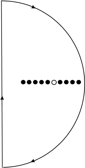
Figure 1: The schematic plot of complex values of each $R_{j}$. Filled circles show locations of energy levels for free electrons. Open circle indicates a missing (blocked) level. Solid line corresponds to the integration path for each $R_{j}$.

At this stage, we substitute equation (7) to equation (8) and integrate using residues. We easily get

$$Z=\exp(-2N\varepsilon_{F_{0}}/V)z,$$ (10)

where

$$z=\sum_{n_{1},n_{2}...,n_{N}=0}^{N_{\Omega}}\left(\prod_{j=1}^{N}(-1)^{n_{j}}\sigma^{n_{j}}\binom{N_{\Omega}}{n_{j}}(n_{j}-n_{\mathbf{p}})\right)\left(\prod_{l,j,l>j}(n_{l}-n_{j})^{2}\right),$$ (11)

where $\sigma=\exp(-2/v)$.

3.2 Vandermonde determinants

It is known that $\prod_{l,j,l>j}(n_{l}-n_{j})$ entering equation (11) can be represented as the determinant of the Vandermonde matrix

$$\prod_{l,j,l>j}(n_{l}-n_{j})\equiv V_{0}(\left\{n_{j}\right\})=\det\begin{bmatrix}1&1&1&\ldots&1\\ n_{1}&n_{2}&n_{3}&\ldots&n_{N}\\ n_{1}^{2}&n_{2}^{2}&n_{3}^{2}&\ldots&n_{N}^{2}\\ \ldots&\ldots&\ldots&\ldots&\ldots\\ n_{1}^{N-1}&n_{2}^{N-1}&n_{3}^{N-1}&\ldots&n_{N}^{N-1}\end{bmatrix}.$$ (12)

Consequently, we can rewrite the total product $\prod_{l,j,l>j}(n_{l}-n_{j})^{2}$ as
$(-1)^{N(N-1)/2}V_{0}(\left\{{n_{j}}\right\})V_{0}(\left\{N_{\Omega}-n_{j}\right\})$.

Instead of the standard monomials, we represent $V_{0}(\left\{{n_{j}}\right\})$ in terms of Pochhammer symbols $(n)_{a}=n(n-1)...(n-a+1)$, while $(n)_{0}\equiv 1$. This can be done by iterative substraction of rows of Vandermonde matrix, which does not change the determinant and ultimately leads to

$$V_{0}(\left\{{n_{j}}\right\})=\det\begin{bmatrix}(n_{1})_{0}&(n_{2})_{0}&(n_{3})_{0}&\ldots&(n_{N})_{0}\\ (n_{1})_{1}&(n_{2})_{1}&(n_{3})_{1}&\ldots&(n_{N})_{1}\\ (n_{1})_{2}&(n_{2})_{2}&(n_{3})_{2}&\ldots&(n_{N})_{2}\\ \ldots&\ldots&\ldots&\ldots&\ldots\\ (n_{1})_{N-1}&(n_{2})_{N-1}&(n_{3})_{N-1}&\ldots&(n_{N})_{N-1}\end{bmatrix},$$ (13)

while $V_{0}(\left\{N_{\Omega}-n_{j}\right\})$ can be represented in a similar form with $n_{j}$ changed into $N_{\Omega}-n_{j}$.

Next, we insert $(n_{j}-n_{\mathbf{p}})$, which appears in equation (11), into the Vandermonde matrix in the following manner

$$\left(\prod_{j=1}^{N}(n_{j}-n_{\mathbf{p}})\right)\left(\prod_{j,l,l>j}(n_{l}-n_{j})\right)$$

$$=\det\begin{bmatrix}(n_{1})_{0}(n_{1}-n_{\mathbf{p}})&(n_{2})_{0}(n_{2}-n_{\mathbf{p}})&\ldots&(n_{N})_{0}(n_{N}-n_{\mathbf{p}})\\ (n_{1})_{1}(n_{1}-n_{\mathbf{p}})&(n_{2})_{1}(n_{2}-n_{\mathbf{p}})&\ldots&(n_{N})_{1}(n_{N}-n_{\mathbf{p}})\\ \ldots&\ldots&\ldots&\ldots\\ (n_{1})_{N-1}(n_{1}-n_{\mathbf{p}})&(n_{2})_{N-1}(n_{2}-n_{\mathbf{p}})&\ldots&(n_{N})_{N-1}(n_{N}-n_{\mathbf{p}})\end{bmatrix}$$ (14)

Let us now extract $n_{\mathbf{p}}$ from the first row of the above matrix as

$$\det \begin{bmatrix}(n_{1})_{1}&(n_{2})_{1}&\ldots&(n_{N})_{1}\\ (n_{1})_{1}(n_{1}-n_{\mathbf{p}})&(n_{2})_{1}(n_{2}-n_{\mathbf{p}})&\ldots&(n_{N})_{1}(n_{N}-p)\\ \ldots&\ldots&\ldots&\ldots\\ (n_{1})_{N-1}(n_{1}-n_{\mathbf{p}})&(n_{2})_{N-1}(n_{2}-n_{\mathbf{p}})&\ldots&(n_{N})_{N-1}(n_{N}-n_{\mathbf{p}})\end{bmatrix}$$

$$-n_{\mathbf{p}} \det \begin{bmatrix}(n_{1})_{0}&(n_{2})_{0}&\ldots&(n_{3})_{0}\\ (n_{1})_{1}(n_{1}-n_{\mathbf{p}})&(n_{2})_{1}(n_{2}-n_{\mathbf{p}})&\ldots&(n_{N})_{1}(n_{N}-n_{\mathbf{p}})\\ \ldots&\ldots&\ldots&\ldots\\ (n_{1})_{N-1}(n_{1}-n_{\mathbf{p}})&(n_{2})_{N-1}(n_{2}-n_{\mathbf{p}})&\ldots&(n_{N})_{N-1}(n_{N}-n_{\mathbf{p}})\end{bmatrix}$$ (15)

$$\equiv D_{1}-n_{\mathbf{p}}D_{2}.$$

The first term, $D_{1}$, can be rewritten as

$$D_{1}=\det\begin{bmatrix}(n_{1})_{1}&(n_{2})_{1}&\ldots&(n_{3})_{1}\\ (n_{1})_{2}&(n_{2})_{2}&\ldots&(n_{N})_{2}\\ \ldots&\ldots&\ldots&\ldots\\ (n_{1})_{N-1}(n_{1}-n_{\mathbf{p}})&(n_{2})_{N-1}(n_{2}-n_{\mathbf{p}})&\ldots&(n_{N})_{N-1}(n_{N}-n_{\mathbf{p}})\end{bmatrix}$$ (16)

$$-(n_{\mathbf{p}}-1)\det\begin{bmatrix}(n_{1})_{1}&(n_{2})_{1}&\ldots&(n_{N})_{1}\\ (n_{1})_{1}&(n_{2})_{1}&\ldots&(n_{N})_{1}\\ \ldots&\ldots&\ldots&\ldots\\ (n_{1})_{N-1}(n_{1}-n_{\mathbf{p}})&(n_{2})_{N-1}(n_{2}-n_{\mathbf{p}})&\ldots&(n_{N})_{N-1}(n_{N}-n_{\mathbf{p}})\\ \end{bmatrix}$$

where we have extracted $n_{\mathbf{p}}-1$ from the second row of the initial matrix. We immediately see that the last determinant is exactly zero, since two rows of its matrix are the same. We then extract $n_{\mathbf{p}}-2$ from the third row of the remaining matrix in the RHS of equation (3.2) and repeat our arguments. We follow a similar iterative procedure for $D_{2}$. It is rather straightforward to see that only terms proportional to $(n_{\mathbf{p}})_{m}$ do survive at the end, since all the other terms are proportional to determinants of matrices with repeating rows. We finally arrive to the following identity

$$\left(\prod_{j=1}^{N}(n_{j}-n_{\mathbf{p}})\right)\left(\prod_{j,l,l>j}(n_{l}-n_{j})\right)=\sum_{m=0}^{N}(-1)^{m}(n_{\mathbf{p}})_{m}V_{N-m}(\left\{{n_{j}}\right\})$$ (17)

where $V_{m}(\left\{{n_{j}}\right\})$ are determinants of the matrices, which are obtained from the matrix of the RHS of equation (13) by increasing indices of Pochhammer symbols in the last $m$ rows by one, as $(n_{j})_{a}\rightarrow(n_{j})_{a+1}$.

3.3 Auxiliary identities

To go further, we provide some auxiliary identities, which are going to greatly facilitate calculations. The starting identity is

$$z_{a,b}\equiv\sum_{n=0}^{N_{\Omega}}(-1)^{n}\sigma^{n}\binom{N_{\Omega}}{n}(n)_{a}(N_{\Omega}-n)_{b}=\sigma^{a}(1-\sigma)^{N_{\Omega}-a-b}(-1)^{a}\frac{N_{\Omega}!}{(N_{\Omega}-a-b)!},$$ (18)

where $a+b\leq N_{\Omega}$. It can be obtained by observation that first $a$ terms, as well as last $b$ terms of the initial sum are zero, and then by replacing Pochhammer symbols by ratios of factorials.

Let us now focus on a product of sums for each $n_{j}$, every sum being similar to the one of equation (18). We can write such a product as

$$z_{a_{1},b_{1}}...z_{a_{N},b_{N}} = \sigma^{\sum_{j=1}^{N}a_{j}}(1-\sigma)^{NN_{\Omega}-\sum_{j=1}^{N}(a_{j}+b_{j})}(-1)^{\sum_{j=1}^{N}a_{j}}$$

$$\times\prod_{j=1}^{N}\frac{N_{\Omega}!}{(N_{\Omega}-a_{j}-b_{j})!}.$$ (19)

The dependence of this quantity on $V$ (via $\sigma$) is through two first factors. Their dependencies on sets ${a_{j}}$ and ${b_{j}}$ is only by $\sum_{j=1}^{N}a_{j}$ and $\sum_{j=1}^{N}b_{j}$, which actually are degrees of polynomials $\prod_{j=1}^{N}(n_{j})_{a_{j}}$ and $\prod_{j=1}^{N}(N_{\Omega}-n_{j})_{b_{j}}$, respectively.

3.4 ’Partition function’: hypergeometric series

Let us substitute equation (17) back to equation (11). To proceed in calculations, we have to consider products of the form $V_{m}(\left\{{n_{j}}\right\})V_{0}(\left\{N_{\Omega}-n_{j}\right\})$. It is easy to see from equation (13) that each of them (for a given $m$) can be represented as a linear combination of polynomials of the form $\left(\prod_{j=1}^{N}(n_{j})_{a_{j}}\right)\left(\prod_{j=1}^{N}(N_{\Omega}-n_{j})_{b_{j}}\right)$ with the unique $\sum_{j=1}^{N}a_{j}=m+N(N-1)/2$ and $\sum_{j=1}^{N}b_{j}=N(N-1)/2$ for each polynomial. These two numbers just give the degrees of the polynomials $V_{m}(\left\{{n_{j}}\right\})$ and $V_{0}(\left\{N_{\Omega}-n_{j}\right\})$, respectively. According to equation (19), after substitution of these products to equation (11) and performing summations, we get the same dependence of the result on $\sigma$ for any of these polynomials (at a given $m$). Hence, we can write

$$z=\sigma^{N(N+1)/2}\left(1-\sigma\right)^{N(N_{\Omega}-N)}\sum_{m=0}^{N}(n_{\mathbf{p}})_{m}\left(\sigma^{-1}-1\right)^{m}\alpha_{m},$$ (20)

where $\alpha_{m}$ are unknown numbers independent on $\sigma$, which have a combinatorial origin.

We avoid a direct calculation of ${\alpha_{m}}$ by using a trick, which is based on the well-known rule: $\binom{N_{\Omega}}{n}=\binom{N_{\Omega}}{N_{\Omega}-n}$. Namely, we change summation variables in equation (11) as $n_{j}^{{}^{\prime}}=N_{\Omega}-n_{j}$. It is then readily seen that

$$z(n_{\mathbf{p}},\sigma)=(-1)^{N+NN_{\Omega}}\sigma^{NN_{\Omega}}z(N_{\Omega}-n_{\mathbf{p}},\sigma^{-1}).$$ (21)

For $z(N_{\Omega}-n_{\mathbf{p}},\sigma^{-1})$ we can use equation (20) with $n_{\mathbf{p}}\rightarrow N_{\Omega}-n_{\mathbf{p}}$, $\sigma\rightarrow\sigma^{-1}$. By doing this, we arrive to another expression of $z(n_{\mathbf{p}},\sigma)$ in terms of $(N_{\Omega}-n_{\mathbf{p}})_{m}$, which is nevertheless equivalent to equation (20):

$$z=\sigma^{N(N-1)/2}\left(1-\sigma\right)^{N(N_{\Omega}-N)}\sum_{m=0}^{N}(N_{\Omega}-n_{\mathbf{p}})_{m}\left(\sigma^{-1}-1\right)^{m}\alpha_{m}.$$ (22)

The idea is to express Pochhammer symbols of $N_{\Omega}-n_{\mathbf{p}}$ in terms of Pochhammer symbols of $n_{\mathbf{p}}$, then to substitute them to equation (22) and to compare the result with equation (20). By equating coefficients of Pochhammer symbols of $n_{\mathbf{p}}$, we are going to obtain a system of linear equations for $\left\{\alpha_{m}\right\}$. We make use of the following relation

$$(N_{\Omega}-n_{\mathbf{p}})_{m}=\sum_{l=0}^{m}(-1)^{l}(n_{\mathbf{p}})_{l}\binom{m}{l}\frac{(N_{\Omega}-l)!}{(N_{\Omega}-m)!},$$ (23)

which can be trivially checked for $m=0,$ $1$ and then proved by induction. Inserting it to equation (22) and solving the system of equations for $\left\{\alpha_{m}\right\}$, we get

$$\alpha_{m}=\alpha\binom{N}{m}\frac{1}{(N_{\Omega})_{m}},$$ (24)

where $\alpha$ is an irrelevant constant, independent on $\sigma$.

Finally, we obtain $z$ as

$$z = \alpha\sigma^{N(N+1)/2}\left(1-\sigma\right)^{N(N_{\Omega}-N)}z^{\prime},$$ (25)

where

$$z^{\prime}=\sum_{m=0}^{N}\binom{N}{m}\frac{(n_{\mathbf{p}})_{m}}{(N_{\Omega})_{m}}\left(\sigma^{-1}-1\right)^{m}.$$ (26)

The last expression can be considered as a hypergeometric series.

3.5 Hypergeometric series: saddle-point method

Actually, equation (25) already allows us to find $E_{R,\textbf{p}}$ in terms of the hypergeometric series. The resulting expression, however, is essentially untractable from the perspective of a further analysis. Let us, therefore, try to transform $z^{\prime}$ into a simpler form.

We note that, for natural numbers $n_{\mathbf{p}}$ and $m$, $(n_{\mathbf{p}})_{m}=0$ for any $m$, which is larger than $n_{\mathbf{p}}$. Hence, we can change the upper limit of summation in equation (26) to $\min(n_{\mathbf{p}},N)$. After that, all the terms in the sum are nonzero, so that we can replace Pochhammer symbols of $n_{\mathbf{p}}$ by ratios of factorials, as $(n_{\mathbf{p}})_{m}=n_{\mathbf{p}}!/(n_{\mathbf{p}}-m)!$.

We also see that $\sigma^{-1}-1\equiv\exp(2/v)-1$ is always positive. The last circumstance is very important: it means that terms in the sum are not oscillating in sign. Therefore, we can switch from summation to integration. We also utilize asymptotic expansion for factorials entering both Pochhammer symbols and the binomial coefficient, since we are interested in macroscopic numbers, $\sim N$. Note that the important case of $n_{\mathbf{p}}=0$ must be considered as $n_{\mathbf{p}}=0\times N$, although this particular situation can be analyzed separately without switching to integration, since the derivation turns out to be quite simple (the results of both approaches are finally the same). After straightforward algebra, we arrive to the identity

$$z^{\prime}\simeq\int_{0}^{\min(n_{\mathbf{p}},N)}e^{H(m)}dm,$$ (27)

where

$$H(m)=(N_{\Omega}-m)\ln(N_{\Omega}-m)-m\ln(m)-(N-m)\ln(N-m)$$

$$-(n_{\mathbf{p}}-m)\ln(n_{\mathbf{p}}-m)+m\ln\left(\sigma^{-1}-1\right).$$ (28)

To avoid possible confusion, we note that in equation (27) we have dropped, as usual, an irrelevant $V$-independent prefactor.

In order to evaluate the integral in the RHS of equation (27), we use a saddle-point method. It is straightforward to prove that $H(m)$ has a single maximum within the integration range, which is attained at

$$m_{0}=\frac{1}{2}\ \left\{(n_{\mathbf{p}}+N)(1-\sigma)+N_{\Omega}\sigma\ \right\}$$

$$\times\left\{1-\sqrt{1-\frac{4n_{\mathbf{p}}N(1-\sigma)}{((n_{\mathbf{p}}+N)(1-\sigma)+N_{\Omega}\sigma)^{2}}}\right\}.$$ (29)

We can also ensure that the position of this maximum is far enough from both integration limits, since $H^{\prime\prime}(m_{0})\sim N^{-1}$, while $1/\sqrt{H^{\prime\prime}(m_{0})}\sim\sqrt{N}$ determines the width of the neighborhood of $m_{0}$, which gives the dominant contribution to the integral. At the same time, both $m_{0}$ and $(\min(n_{\mathbf{p}},N)-m_{0})$ do scale as $N$. Together with the fact that $H^{(n)}(m_{0})\sim N^{-n+1}$ at $n>2$, this enables us to reduce the problem to the simple Gaussian integration. Keeping leading order in $N$, we obtain

$$\ln z^{\prime}=H(m_{0}).$$ (30)

By finding a logarithmic derivative of $z$, given by equation (25), and by adding the kinetic energy of the unpaired electron $\varepsilon_{F0}+n_{\textbf{p}}/\rho$, we arrive to the expression of the total energy $E_{N,\textbf{p}}$ of the system of $N$ pairs and one unpaired electron. After some simple algebra and using the known expression for the ground state energy[12] $E_{N}$, we can present $E_{N,\textbf{p}}$ as

$$E_{N,\textbf{p}}=E_{N}+\mu+\sqrt{\Delta^{2}+(\varepsilon_{\mathbf{p}}-\mu)^{2}},$$ (31)

while

$$\Delta=\frac{2}{\rho}\frac{\sqrt{\sigma}}{1-\sigma}\sqrt{N(N_{\Omega}-N)},$$ (32)

$$\mu=\varepsilon_{F0}+\frac{N}{\rho}\frac{1+\sigma}{1-\sigma}-\Omega\frac{\sigma}{1-\sigma}.$$ (33)

Physical meanings of $\Delta$ and $\mu$ will be fixed below.

The formalism presented above is restricted to $N\leq N_{\Omega}/2$. In order to address configurations with $N>N_{\Omega}/2$, we switch to holes. It is then straightforward to ensure that equation (31) still holds in this case.

4 Discussion

We now consider $E_{N,\textbf{p}}$ as a function of $\varepsilon_{p}$. In particular, it is of interest to determine the lowest possible $E_{N,\textbf{p}}$.

First of all, we see that $\mu$, given by equation (33), can be actually considered as a chemical potential. Indeed, by calculating $(E_{N}-E_{N-1})/2$, we find that this quantity does coincide with $\mu$.

The minimum value of $E_{N,\textbf{p}}$ is attained at $n_{\mathbf{p}}$, which gives a minimum of $(\varepsilon_{\textbf{p}}-\mu)^{2}$, provided that $n_{\mathbf{p}}$ is confined between 0 and $N_{\Omega}$. If $\mu-\varepsilon_{F0}$ also falls into this range, one can always choose $n_{\mathbf{p}}/\rho=\mu-\varepsilon_{F0}$, so that $(\varepsilon_{\textbf{p}}-\mu)^{2}$ is zero, while the square root in the RHS of equation (31) reduces to $\Delta$. It is easy to see that for the half-filling configuration, $N_{\Omega}=N/2$, the expression of $\Delta$, as given by equation (32), reproduces precisely the BCS formula for the gap. This conclusion is also in agreement with the result of the traditional method to solve Richardson equations in the large-sample limit, which uses an assumption that energy-like quantities are arranged into arcs on the complex plane.[11, 20, 21]  The assumption on arcs is actually deduced from numerical solutions of Richardson equations, so that, in general case, it is not fully controllable, from our point of view. Similar approach is also widely used in a broader context for the solution of the Bethe-ansatz equations.[22]  Another method,[13]  which is based on Taylor expansions of sums appearing in Richardson equations around the known single-pair solution, up to now has been successfully applied to the ground state only, while its application to excited states leads to heavy mathematical problems.

If the chemical potential goes below the lower cutoff $\varepsilon_{F0}$, i.e., $\mu-\varepsilon_{F0}$ becomes negative, a constrained minimum of $E_{N,\textbf{p}}$ corresponds to $n_{\mathbf{p}}=0$. By solving the equation $\mu-\varepsilon_{F0}=0$, we see that the transition between the two regimes occurs at $N=N_{0}$, where

$$N_{0}=N_{\Omega}\frac{\sigma}{1+\sigma}.$$ (34)

If the chemical potential goes above the upper limit of the potential layer, the minimum energy corresponds to $\varepsilon_{p}$ located at this upper limit. By solving the equation $\mu-\varepsilon_{F0}=\Omega$, we find that the transition to this regime happens at $N_{\Omega}-N_{0}$. This result is in agreement with the electron-hole symmetry.

Thus, for the minimum of $E_{N,\textbf{p}}$, we have three regimes

$$\min(E_{N,\textbf{p}})=E_{N}+\mu+\left(\frac{N}{\rho}+\Omega\frac{\sigma}{1-\sigma}\right),$$ (35)

at $N\leq N_{0}$;

$$\min(E_{N,\textbf{p}})=E_{N}+\mu+\Delta,$$ (36)

at $N_{0}<N<N_{\Omega}-N_{0}$;

$$\min(E_{N,\textbf{p}})=E_{N}+\mu+\left\{\left(\Omega-\frac{N}{\rho}\right)+\Omega\frac{\sigma}{1-\sigma}\right\},$$ (37)

at $N_{\Omega}-N_{0}\leq N$.

In the weak-coupling limit, $\sigma\ll 1$, we have: $N_{0}\simeq N_{\Omega}\sigma$. This value actually corresponds to the density of pairs, at which their wave functions start to overlap. Such an overlap can be considered as a signature of the transition from the isolated-pair regime to the dense condensate.

In the dilute regime, $N<N_{0}$, the excitation energy is controlled by $\Omega\sigma/(1-\sigma)$, which is nothing but half the binding energy $\epsilon_{c}$ of an isolated pair.[13]  In the dense regime, $N_{\Omega}-N_{0}\geq N>N_{0}$, it is governed by the BCS gap $\Delta$, which has to be considered as a collective many-body response of the system to the appearance of one blocked level. It is of interest to note that pair binding energy and the gap have similar, but different dependencies on interaction constant $v$. Namely, in the weak-coupling limit, the first quantity is proportional to $exp(-2/v)$, while the second one behaves as $\sim exp(-1/v)$ due to equation (32). This equation also shows that $\Delta$ is symmetric with respect to the mutual replacement of electron and holes, so that the electron-hole symmetry again shows up. The third regime can be considered as a ’superdense’ regime of Cooper pairs, made of electrons, or the dilute regime of Cooper pairs, made of holes. In this regime, we again see a single-pair binding energy appearing in $\min(E_{N,\textbf{p}})$. It can be now understood as a binding energy of a pair made out of holes.

Thus, we have identified three regimes for the energy difference between $E_{N,\textbf{p}}$ and $E_{N}$ depending on the energy layer filling. These are a dilute regime of pairs, BCS regime, and a dilute regime of holes. With changing layer filling, transitions between these regimes occur smoothly. We have found that only higher-order derivatives of $E_{N,\textbf{p}}$ with respect to $N$ experience discontinuities upon the transitions.

Up to now, we considered states with only one unpaired electron. Let us address the energy of the state with two such electrons. This should allow us to make a comparison with the energy of the system with all the electrons paired, the total number of particles being conserved. In principle, in order to find the energy, we should perform similar calculations, but with two states blocked. However, we may use a simple trick allowing one to avoid making such computations. It is rather obvious that it is energetically favorable for the two unpaired electrons to occupy two neighboring states rather than to be separated. We then come back to the electrostatic picture and perform a coarse-graining of the initial configuration. Namely, we merge couples of neighboring fixed particles, as well as couples of neighboring free particles into ’superparticles’ with charges being twice larger than initial ones. We must also increase by a factor of two a homogeneous forces acting on free charges. This procedure does not change dominant (extensive) contribution of the total energy. Within this procedure, two blocked states are converted into a single one, so that we can map this picture to the above situation. By doing this, after some straightforward calculations, we finally reach an expectable result: the difference of energies of the states with $N$ pairs and $N-1$ pairs plus two unpaired electrons is twice the square root entering RHS of (31).

Finally, let us discuss another type of excited states, which corresponds to one of the energy-like quantities trapped between two one-electronic levels. The energy of such a state can be again handled using electrostatic analogy without making detailed calculations. Namely, we note that the role of the free charge trapped is to compensate two fixed charges, between which it is accommodated, since each of them has an opposite charge, but twice smaller in absolute value. We again map this configuration to the previous one with two states blocked and find the same gap, within dominant terms in $1/N$.

5 Conclusions

Richardson equations provide an exact solution for the BCS pairing Hamiltonian. These equations are deterministic and posses a well-known electrostatic analogy. Therefore, one can convert the problem of their resolution to the probabilistic problem, as it was recently suggested in Ref. Pogosov for the ground state of the initial quantum problem. This approach avoids assumption that Richardson solutions in the large-$N$ limit are arranged in arcs on the complex plane.

In the present paper, we applied this treatment to excited states with the focus on the equally-spaced model and the thermodynamical limit. We have considered arbitrary fillings of the energy interval, where the attractive potential acts. The ’partition function’ for the deterministic problem has been found analytically by converting the Selberg-type integral into coupled binomial sum, evaluated using combinatorial properties of Vandermonde matrix.

For the energy difference between the first excited state and the ground state (energy gap), three regimes have been identified, which can be considered as the dilute regime of pairs, BCS regime, and dilute regime of holes. Explicit expressions have been derived. Transitions between these regimes occur smoothly, accompanied by only weak singularities. The results supports the BCS result for the half-filling.

References

- [1] J. Bardeen, L. N. Cooper, and J. R. Schrieffer, Phys. Rev. 108 (1957), 1175.
-
[2]
N. N. Bogoliubov, ZhETF 34 (1958), 58 [Sov. Phys. JETP 7
(1958), 41].
N. N. Bogoliubov, Nuovo Cimento 7 (1958), 794. - [3] J. R. Schrieffer, Theory of Superconductivity (Perseus Books Group, Massachusetts, 1999).
-
[4]
R. W. Richardson, Phys. Lett. 3 (1963), 277.
R. W. Richardson and N. Sherman, Nucl. Phys. 52 (1964), 221. - [5] J. von Delft and R. Poghossian, Phys. Rev. B 66 (2002), 134502.
- [6] M. Gaudin, J. Phys. (Paris) 37 (1976), 1087.
- [7] M. Asorey, F. Falceto, and G. Sierra, Nucl. Phys. B 622 (2002), 593.
- [8] J. Dukelsky, S. Pittel, and G. Sierra, Rev. Mod. Phys. 76 (2004), 643.
- [9] F. Braun and J. von Delft, Phys. Rev. Lett. 81 (1998), 4712.
-
[10]
L. Amico and A. Osterloh, Phys. Rev. Lett. 88 (2002),
127003.
H.-Q. Zhou, J. Links, R. H. McKenzie, and M. D. Gould, Phys. Rev. B 56 (2002), 060502(R).
A. Faribault, P. Calabrese, and J.-S. Caux, Phys. Rev. B 77 (2008), 064503.
G. Gorohovsky and E. Bettelheim, Phys. Rev. B 84 (2011), 224503. - [11] R. W. Richardson, J. Math. Phys. 18 (1977), 1802.
- [12] W. V. Pogosov, J. Phys.: Condens. Matter 24 (2012), 075701.
-
[13]
W. V. Pogosov and M. Combescot, Pis’ma v ZhETF 92 (2010), 534 [JETP Letters 92
(2010), 534].
M. Crouzeix and M. Combescot, Phys. Rev. Lett. 107 (2011), 267001. - [14] A. J. Leggett, J. de Physique. Colloques 41 (1980), C7.
- [15] D. M. Eagles, Phys. Rev. 186 (1969), 456.
- [16] I. Snyman and H. B. Geyer, Phys. Rev. B 73 (2006), 144516.
- [17] Q. Chen, J. Stajic, S. Tan, and K. Levin, Physics Reports 412 (2005), 1.
- [18] V. F. Gantmakher and V. T. Dolgopolov, Usp. Fiz. Nauk 180 (2010), 3.
- [19] A. Zabrodin and P. Wiegmann, J. Phys. A 39 (2006), 8933.
- [20] J. M. Roman, G. Sierra, and J. Dukelsky, Nucl. Phys. B 634 (2002), 483.
- [21] E. A. Yuzbashyan, A. A. Baytin, and B. L. Altshuler, Phys. Rev. B 71 (2005), 094505.
- [22] V. A. Kazakov, A. Marshakov, J. A. Minahan and K. Zarembo, J. High Energy Phys. 405 (2004), 024.