Inter-Coder Agreement for Nominal Scales: A Model-based Approach

Abstract

Inter-coder agreement measures, like Cohen’s $\kappa$, correct the relative frequency of agreement between coders to account for agreement which simply occurs by chance. However, in some situations these measures exhibit behavior which make their values difficult to interprete. These properties, e.g. the “annotator bias” or the “problem of prevalence”, refer to a tendency of some of these measures to indicate counterintuitive high or low values of reliability depending on conditions which many researchers consider as unrelated to inter-coder reliability. However, not all researchers agree with this view, and since there is no commonly accepted formal definition of inter-coder reliability, it is hard to decide whether this depends upon a different concept of reliability or simply upon flaws in the measuring algorithms.

In this note we therefore take an axiomatic approach: we introduce a model for the rating of items by several coders according to a nominal scale. Based upon this model we define inter-coder reliability as a probability to assign a category to an item with certainty. We then discuss under which conditions this notion of inter-coder reliability is uniquely determined given typical experimental results, i.e. relative frequencies of category assignments by different coders.

In addition we provide an algorithm and conduct numerical simulations which exhibit the accuracy of this algorithm under different model parameter settings.

1 Introduction

Measuring the agreement between the nominal ratings of a set of items by several coders or judges is a common task in a number of disciplines like medical, psychological, and social sciences, content analysis and marketing. Simply measuring the percentage of agreement is not adequate as it does not take into account agreement which simply occurs by chance. There have been proposed a number of inter-coder reliability measures to cope with this effect, the most prominent being $\kappa$ [5], $\pi$ ([14], [8]), $\alpha$ [13], and $S$ [3], see [2] for a survey.

These measures are defined as ratios of chance-corrected numbers of observed agreement vs. maximal agreement and differ in the way the chance-correction is taken into account. The ways these corrections are computed, give rise to some criticism of these measures, because they “favor” or “penalize” certain coder behaviors which are considered as inappropriate by some researchers.

Though usually not explicitly stated (cf. also [1, p. 294]), the basic assumption is that a coder either assigns a category by certainty resp. “expert judgment” (Brennan and Prediger, [4, p. 689]) or assigns some category without being absolutely sure about his or her choice. Obviously, it is not possible for an individual assignment to identify whether the assignment was done by certainty or not, sometimes not even the rater himself or herself may be sure about what the exact reasons for his or her choice are.

At one extreme point is the $S$-value which assumes a uniform distribution of categories when “chance assignments” occurs. Scott’s $\pi$ and Cohen’s $\kappa$ on the other hand use “marginal distributions”, i.e. the overall distribution of category assignments by each rater, to correct for chance agreement. Using marginal distributions may lead to incorrect chance correction since these distributions also include assignments made by certainty and thus may also be more than marginally influenced by the distribution of categories according to the population of items. Using uniform distribution on the other hand may underestimate chance agreement if there are categories that coders hardly ever choose. There exists a considerable literature on this subject, see e.g. [2], [4], [6], [7], [9],[11] [12].

Obviously it is hard to reach at a consensus about which strategy a coder will follow in general when category assignment is not done by certainty. In our model we thus will not presume a certain distribution to account for chance agreement.

Cohen’s $\kappa$ exhibits a feature, usually called “annotator bias” which describes the fact that $\kappa$ yields higher values when coders produce widely diverging marginal distributions than when the marginal distributions are similar. See [2, section 3.1] who support this feature, [6], [7],[17] for criticism, [15] for a formal proof. Scott’s $\pi$, in contrast, uses the common marginal distribution of the coders and so “favors” coders that produce similar marginal distributions.

In order to measure inter-coder reliability (in contrast to intra-coder, i.e. test-retest reliability) it is necessary that the experiment can be reproduced when conducted in the same way with another group of coders (which of course may be restricted to a certain base population e.g. trained in some way, but not delimited to some particular individuals). So an inter-coder reliability measure should (approximately) yield the same value for every sufficiently large subset of coders from the prescribed population of coders and the coders’ marginal distributions may vary according to some distribution which depends on the population of coders.

Another debated fact is the prevalence problem, referring to the fact that some of these measures ($\kappa$,$\pi$,$\alpha$) produce low scores when one category is predominant among the ratings (see [2], [6], [7], [9] for examples and discussion).

There is some debate on this issue. While [6], [7] and [9] consider this as a weakness, it is justified by Artstein and Poesio with the argument that “reliability in such cases is the ability to agree on rare categories” [2, section 3.2]. This latter argument is somewhat problematic for statistical measures which usually are designed to exhibit typical not exceptional behavior. In our model we will take an approach which defines reliability as a property common to the category assignments and independent of the relative frequency of the (“true” or “correct”) items’ categories. However it will turn out that reliability can only be determined if not all items belong to one category.

The approach we take differs from these measures as we start with an axiomatic model-based definition of inter-coder reliability, which will be a probability of some event. This has the nice side effect that the value of the reliability parameter can be stated as a probability of an idealized coder’s behavior and thus has a direct interpretation.

In addition basing the definition of inter-coder reliability upon such a model one may simulate coder ratings with a known reliability parameter and thus may evaluate the accuracy of algorithms under different setups. We will do this in Section 4 for the algorithm we provide.

Though the author believes that the model used here is fairly general, there might be situations in which it could be deemed unfeasible. Here the explicit statement of the model’s assumptions helps to determine whether the model is acceptable in an experiment or not. We will take a closer look at some of the assumptions of the model and their possible impact on reliability results at the end of the next section.

2 The Model

We denote by $C=\{c_{1},\ldots,c_{m}\}$ the (finite) set of $m$ categories, into which $N$ items, $\mathbb{N}_{N}$, are to be classified by the $R$ raters, $\mathbb{N}_{R}$. We use $\mathbb{N}_{n}$ to denote the natural numbers $\{1,\ldots,n\}$.

The common assumptions for inter-rater agreement are (rephrased from [5]):

1. The items are independent

2. The categories are independent, mutually exclusive, and exhaustive.

3. The raters operate independently

Assumption (ii) that categories are exhaustive and mutually exclusive implies that for every item there is one and only one “correct” category. In other words, assumption (ii) above implies the existence of a (usually unknown) function

$$\gamma\,:\,\mathbb{N}_{N}\rightarrow C.$$

We will sometimes call $\gamma(k)$ the “true” category associated with item $k$, without any philosophical implication of the term “true”.

For each $c\in C$ let $N_{c}:=\#\gamma^{-1}(c)$ denote the number of items whose true category is $c$, and write $\tau_{c}:=\frac{N_{c}}{N}$ for the relative frequency of these items.

If a coder rates an item he or she may either be sure about the category to be chosen or not. If the coder is sure about the item’s category it seems natural to assume that the coder will assign this category to the item (so we assume that the coders will not cheat but will assign a category to the best of their knowledge).

Now, what happens in the case the coder is not completely sure about the category to assign? In this case, considering a large set of such items, we will observe a certain relative frequency for the categories to be chosen. In general it is hard to know which strategy the coder will take and this is frequently debated in the context of Cohen’s $\kappa$. Coders might follow some “base rate” i.e. are guided by some assumption about the distribution of categories in the population of items, or may choose the category according to a uniform distribution on the set of categories (cf. e.g. [3], [11]).

There are certainly good reasons for many of these assumptions and it is probably also dependent upon the field of research (e.g. medical diagnosis vs. speech analysis), upon the kinds of items, the professional background and education of the raters (e.g. scholars vs. laymen) and many more properties. Hence we will not assume any particular distribution but only assume that such a distribution exists.

To formalize we thus assume that given an item $k$ a rater recognizes the true category $\gamma(k)$ with a probability $\beta$. If the coder fails to recognize it he or she assigns a “random” category with some unknown distribution. The assumption (i) above suggests to model these actions by independent random variables.

So formally let $Z_{k}$ be 0-1-valued, $Y_{k}$ be $C$-valued independent random variables $k\in\mathbb{N}_{N}$ and assume that both families are identically distributed.

We define a coder’s rating of item $k\in\mathbb{N}_{N}$ by the outcome of the random variable $X_{k}$ given by

$$X_{k}:=\begin{cases}\gamma(k)&,\text{ if }Z_{k}=0\\ Y_{k}&,\text{ if }Z_{k}=1.\end{cases}$$ (1)

We let $\beta:=\mathbb{P}(Z_{k}=0)$ and $p_{c}:=\mathbb{P}(Y_{k}=c)$.

It is immediate from the definition that

$$\mathbb{P}(X_{k}=c)=\beta\delta_{c,\gamma(k)}+(1-\beta)p_{c},$$ (2)

so the distribution of $X_{i,k}$ is a mixture of the atomic distribution at $\gamma(k)$ and ${\bf p}=(\mathbb{P}^{Y_{k}}(c))_{c\in C}$ with mixture parameter $\beta$. (Here $\delta$ is Kronecker’s delta, i.e. $\delta_{x,y}=1$ if $x=y$ and $0$ otherwise.)

For convenience let us call this model the coder model with parameters $(\beta,\gamma,{\bf p})$, where ${\bf p}=(p_{c})_{c\in C}$. Throughout this note we will tacitly let $\mathbb{N}_{N}$ denote the domain and $C$ the codomain of $\gamma$. A family of independent $C$-valued random variables $(X_{k})_{k\in\mathbb{N}_{N}}$, which satisfies (2) is called a coder process for the coder model.

According to the assumption (iii) above several coders are modeled by independent families $(X_{i,k})_{k\in\mathbb{N}_{N}}$, where the subscript $i$ refers to the coder.

If a rater chooses to assign category $c$ to an item $k$ he or she may either be certain about the items category or may be uncertain and assigns $c$ by chance only. Gwet [10, section 4] uses this same interpretation of the rating process. In our model certainty occurs when the coder chooses the category according to $\gamma(k)$, i.e. when $Z_{k}=0$. So it seems reasonable to use the probability $\beta=\mathbb{P}(Z_{k}=0)$ as agreement indicator, let us call it the reliability parameter of the coder model. Of course an assignment to category $\gamma(k)$ also occurs when $Y_{k}=\gamma(k)$, which happens with probability $p_{\gamma(k)}$.

Aickin [1] also used a mixture model to study inter-coder reliability. In our notation the mixture distribution in Aickin’s model is the distribution

$$(c_{1},c_{2})\mapsto\mathbb{E}(\frac{1}{N}\#\{i\in\mathbb{N}_{N}:X_{i,1}=c_{1}\}\frac{1}{N}\#\{i\in\mathbb{N}_{N}:X_{i,2}=c_{2}\})$$

which is not a mixture distribution in our model, cf. (4), so our model is different from Aickin’s.

There are three features of this model which may need a second look:

The first feature is that coders are modeled by identically distributed families of random variables. This might seem oversimplifying since generally every coder may have his or her own preference. Actually this feature touches the controversy about “annotator bias”.

As we already discussed in the introduction, inter-coder reliability in contrast to intra-coder reliability is only present if the experiment can be reproduced with different coders from some coder population. Our model uses the parameters $\beta$ and ${\bf p}$ to characterize the coder population.

The second feature that may deserve closer consideration, is concerned with the a priori distribution ${\bf p}$ being independent of the item in question. Actually often one may arrive at the situation where for a particular item the coders easily may rule out some categories but are doubtful about some others. In this situation assuming that the a priori distribution is the same for all items is indeed oversimplifying. Without this assumption, however, the model would be completely useless. Indeed, if ${\bf p}$ would be dependent on the item $k$ we could simply put ${\bf p}^{(k)}$ to the distribution of categories obtained for this item and find out that every outcome could be obtained with reliability parameter $\beta=0$, i.e. by pure randomness.

If in some experimental setup the independence of ${\bf p}$ on the item would be deemed a relevant issue, it would be advisable to split the set of items into subsets such that the a priori distribution could be considered the same for all items in each of the subsets.

The third feature which deserves attention is that the probability to identify item $k$ as belonging to category $\gamma(k)$ is independent of $\gamma(k)$, i.e. that $\beta$ is considered independent of $c$. It is easy to imagine a situation where some subset of categories are more easily distinguished from each other than for another subset. In this situation it would indeed be more appropriate to assume $\beta$ to be dependent of $c$. However this would entail the necessity to report several values as reliability parameter, which would make comparisons more difficult.

Even here one should cope with this feature by a careful design of the experiment (choice of categories). We will return to this aspect later (following Proposition 5).

3 Inter-Coder Agreement

According to our model inter-coder reliability is the parameter $\beta$ in (2) which, since $\gamma$ is unknown, is not directly observable in experiments. In experiments only relative frequencies of category assignments can be observed, i.e. we can observe $\frac{1}{N}\#\{i\in\mathbb{N}_{N}:X_{i,1}=c_{1},\ldots{},X_{i,r}=c_{r}\}$ or, idealized, the expectation values of it. In the present section we will discuss under which conditions $\beta$ can be uniquely determined from these expectation values.

Throughout this section we will frequently use the following relations, the proof of which is obvious from (2) and the independence of $X_{i,k}$.

$$e_{1,c} :=\mathbb{E}\left(\frac{1}{N}\#\{k\in\mathbb{N}_{N}:X_{k}=c\}\right)=\beta\tau+(1-\beta)p_{c}$$ (3)

$$e_{2,c_{1},c_{2}} :=\mathbb{E}\left(\frac{1}{N}\#\{k\in\mathbb{N}_{N}:X_{1,k}=c_{1},X_{2,k}=c_{2}\}\right)$$

$$=\beta^{2}\delta_{c_{i},c_{2}}\tau_{c_{1}}+\beta(1-\beta)(\tau_{c_{1}}p_{c_{2}}+\tau_{c_{2}}p_{c_{1}})+(1-\beta)^{2}p_{c_{1}}p_{c_{2}}$$ (4)

$$e_{2,c} :=e_{2,c,c}=\beta^{2}\tau_{c}+2\beta(1-\beta)\tau_{c}p_{c}+(1-\beta)^{2}p_{c}^{2}$$ (5)

$$e_{3,c} :=\mathbb{E}\left(\frac{1}{N}\#\{k\in\mathbb{N}_{N}:X_{1,k}=X_{2,k}=X_{3,k}=c\}\right)$$

$$=\beta^{3}\tau_{c}+3\beta^{2}(1-\beta)\tau_{c}p_{c}+3\beta(1-\beta)^{2}\tau_{c}p_{c}^{2}+(1-\beta)^{3}p_{c}^{3}$$ (6)

Our first result shows that it is not always possible to identify $\beta$ from the coder’s ratings.

Proposition 1

Let $(\beta,\gamma,{\bf p})$ be a coder model and assume that there is $c_{0}\in C$ such that $\gamma(k)=c_{0}$ for all $k\in\mathbb{N}_{N}$. Then for every $\beta^{\prime}\leq\beta+(1-\beta)p_{c_{0}}$ there is a coder model $(\beta^{\prime},\gamma,{\bf p^{\prime}})$ such that

$$\beta\delta_{c,\gamma(k)}+(1-\beta)p_{c}=\beta^{\prime}\delta_{c,\gamma(k)}+(1-\beta^{\prime})p_{c}^{\prime}$$ (7)

for all $c\in C$, $k\in\mathbb{N}_{N}$.

Proof Given $\beta^{\prime}\leq\beta+(1-\beta)p_{c_{0}}$, we only have to show the existence of a vector ${\bf p^{\prime}}\in[0,1]^{m}$ with $\sum_{c\in C}p_{c}=1$ such that (7) holds.

Assume first that $\beta^{\prime}=1$. Then $1=\beta^{\prime}\leq\beta+(1-\beta)p_{c_{0}}\leq 1$ so

$$(1-\beta)(p_{c_{0}}-1)=0$$ (8)

Hence either $\beta=1$ or $p_{c_{0}}=1$. In the first case the statement is trivially satisfied and in the second case we may set $p_{c}^{\prime}=p_{c}$ for all $c\in C$ and obtain either 1 (if $c=c_{0}$) or 0 on both sides of (7), proving the statement in this case.

Now assume $\beta^{\prime}<1$. Then

$$\beta^{\prime} \leq\beta+(1-\beta)p_{c_{0}}=\beta+(1-\beta)(1-\sum_{c\not=c_{0}}p_{c})\leq 1-(1-\beta)p_{c}$$

for all $c\in C\setminus\{c_{0}\}$. Hence $(1-\beta)p_{c}\leq 1-\beta^{\prime}$, so defining

$$p_{c}^{\prime}:=\frac{1-\beta}{1-\beta^{\prime}}p_{c}$$

we obtain $p_{c}^{\prime}\in[0,1]$, for $c\not=c_{0}$. Also define

$$p_{c_{0}}^{\prime}:=\frac{\beta-\beta^{\prime}+(1-\beta)p_{c}}{1-\beta^{\prime}}.$$

Then $p_{c_{0}}^{\prime}\geq 0$ by the condition on $\beta^{\prime}$ and $\beta-\beta^{\prime}+(1-\beta)p_{c}\leq\beta-\beta^{\prime}+(1-\beta)=1-\beta^{\prime}$ shows $p_{c_{0}}^{\prime}\leq 1$. Finally,

$$\sum_{c\in C}p_{c}^{\prime}=p_{c_{0}}^{\prime}+\sum_{c\not=c_{0}}p_{c}^{\prime}=\frac{\beta-\beta^{\prime}}{1-\beta^{\prime}}+\frac{1-\beta}{1-\beta^{\prime}}p_{c_{0}}+\frac{1-\beta}{1-\beta^{\prime}}(1-p_{c_{0}})=1$$

completes the proof. $\Box$

Note that in Proposition 1 we may always choose $\beta^{\prime}=0$, so the rating cannot be distinguished from a completely random one, but of course at the cost of a distribution ${\bf p^{\prime}}$ possibly far from uniform. In the case $\beta=1$, $\beta^{\prime}=0$ the distribution ${\bf p^{\prime}}$ is atomic at $c_{0}$, which somewhat challenges the intuition of “random agreement”.

On the other hand, unless we know that $\#\gamma(\mathbb{N}_{N})>1$, we are actually unable to determine the reliability parameter $\beta$.

Proposition 2

Let $(\beta,\gamma,{\bf p})$ be a coder model and assume that $\tau_{c}<1$ for all $c\in C$. Then the following holds

1. if $e_{2,c_{0}}=e_{1,c_{0}}^{2}$ for some $c_{0}$ then either $\tau_{c_{0}}=0$ or $\beta=0$.

2. $e_{2,c}=e_{1,c}^{2}$ for all $c\in C$ if and only if $\beta=0$

3. if $e_{2,c_{0}}\not=e_{1,c_{0}}^{2}$ for some $c_{0}$ then $e_{2,c_{0}}>e_{1,c_{0}}^{2}$ and

   $$\beta=\sqrt{\frac{e_{2,{c_{0}}}-e_{1,{c_{0}}}^{2}}{\tau_{c_{0}}(1-\tau_{c_{0}})}}$$ (9)

   and $p_{c_{0}}$ is given by

   $$p_{c_{0}}=\frac{e_{1,{c_{0}}}-\beta\tau_{c_{0}}}{1-\beta}$$ (10)

Proof From (3) and (5) for any $c\in C$

$$e_{1,c}^{2}=\beta^{2}\tau_{c}+2\beta(1-\beta)\tau_{c}p_{c}+(1-\beta)^{2}p_{c}^{2}$$

so

$$e_{2,c}-e_{1,c}^{2}=\beta^{2}\tau_{c}(1-\tau_{c})$$ (11)

Since by assumption $\tau_{c}<1$ equation (11) shows part (i). And since $\sum_{c}\tau_{c}=1$ there is $0<\tau_{c_{0}}<1$ for some $c_{0}\in C$ proving part (ii). Solving (11) for $\beta$ and (3) for $p_{c_{0}}$ completes the proof. $\Box$

One application of this result is, that one may determine the range of the distribution $p_{c}$ from the results of a pre-study with a carefully chosen set of items with known “true” categories which meet the assumption $0<\tau_{c}<1$ for all $c\in C$. Once we know the range, i.e. $min_{c\in C}(p_{c})$ and $max_{c\in C}(p_{c})$ of the a priori distribution and can reasonably assume that it does not change for an arbitrary set of items, we can estimate the reliability parameter for arbitrary distribution ${\bf\tau}$ of true categories using the following

Proposition 3

Let $(\beta,\gamma,{\bf p})$ be a coder model, assume that $\pi_{0}\leq p_{c}\leq\pi_{1}<1$ for $c\in C$ and define $e_{2}:=\sum_{c\in C}e_{2,c}$. Then the following estimate holds

$$\sqrt{\frac{max(0,e_{2}-\pi_{1})}{1-\pi_{1}}}\leq\beta\leq\sqrt{\frac{e_{2}-\pi_{0}}{1-\pi_{0}}}$$

Proof From (5) we see that

$$e_{2} =\sum_{c\in C}\left(\beta^{2}\tau_{c}+2\beta(1-\beta)\tau_{c}p_{c}+(1-\beta)^{2}p_{c}^{2}\right)$$ (12)

$$=\beta^{2}+2\beta(1-\beta)\sum_{c\in C}\tau_{c}p_{c}+(1-\beta)^{2}\sum_{c\in C}p_{c}^{2}$$ (13)

Now, since $0\leq\tau_{c}$ we may estimate $\pi_{0}\tau_{c}\leq\;p_{c}\tau_{c}\leq\pi_{1}\tau_{c}$ and $\pi_{0}p_{c}\leq\;p_{c}^{2}\leq\pi_{1}p_{c}$ and since $\sum_{c\in C}\tau_{c}=1=\sum_{c\in C}p_{c}$ thus obtain

$$\pi_{0}=\sum_{c\in C}\pi_{0}\tau_{c}\leq \sum_{c\in C}\tau_{c}p_{c}\leq\pi_{1},\text{ and }$$ (14)

$$\pi_{0}\leq \sum_{c\in C}p_{c}^{2}\leq\pi_{1}$$ (15)

Thus we may $e_{2}$ estimate from below

$$e_{2}\geq\beta^{2}+2\beta(1-\beta)\pi_{0}+(1-\beta)^{2}\pi_{o}=(1-\pi_{0})\beta^{2}+\pi_{0}$$ (16)

(which implies $e_{2}-\pi_{0}>0$) and similarly from above (replacing $\pi_{o}$ by $\pi_{1}$). Since by assumption $1-\pi_{1}>0$ and $1-\pi_{0}>0$ we obtain the desired estimates. $\Box$

Observe, that the preceding proposition does not assume anything about $\tau_{c}$, it even holds if $\tau_{c_{0}}=1$ for some $c_{0}$.

If $p_{c}$ is the uniform distribution we may put $\pi_{0}=\pi_{1}=\frac{1}{m}$ in the preceding result and obtain the equality $\beta^{2}=\frac{e_{2}-\frac{1}{m}}{1-\frac{1}{m}}$ which is the $S$-value of Bennett, Alpert and Goldstein [3].

The $S$-value has been criticized by Scott [14] that it could be increased by adding spurious categories which would never or hardly ever be used. But, as Scott also notes, such a modification would contradict the assumption of uniform distribution for $p_{c}$, hence by such a modification $\beta$ can no longer be determined by the $S$-value formula. We may however use the preceding proposition to obtain estimates for $\beta$: if one adds a category $c_{0}$ that a coder wouldn’t use, the a priori probability $p_{c_{0}}$ is $0$ and so is the minimum, hence we would obtain the inequality

$$\sqrt{\frac{e_{2}-\pi_{1}}{1-\pi_{1}}}\leq\beta\leq\sqrt{e_{2}}.$$

Since $\sqrt{\frac{e_{2}-\pi_{0}}{1-\pi_{0}}}\leq\sqrt{e_{2}}$, adding such a spurious category results in a larger possible interval for $\beta$, i.e. a worse estimate.

If we even know the distribution ${\bf p}$ we are able to compute $\beta$ exactly. The same is true if the a priori probability $p_{c}$ matches the item category distribution $\tau_{c}$. This is the content of the following

Proposition 4

Let $(\beta,\gamma,{\bf p})$ be a coder model and assume that $\tau_{c}<1$ for all $c\in C$.

1. If ${\bf p}$ is known, $\beta$ can be computed as

   $$\beta=\begin{cases}0\text{, if }p_{c}=1\text{ and }e_{1,c}=1\\ \frac{1-2e_{1,c}+e_{2,c}}{1-e_{1,c}}\text{, if }p_{c}=1\text{ and }e_{1,c}<1\\ 1-\frac{1}{2}\left(\frac{1-e_{1,c}}{1-p_{c}}+\frac{e_{1,c}}{p_{c}}\right)+\sqrt{\frac{1}{4}\left(\frac{1-e_{1,c}}{1-p_{c}}+\frac{e_{1,c}}{p_{c}}\right)^{2}-\frac{e_{1,c}-e_{2,c}}{p_{c}(1-p_{c})}}\text{, if }0<p_{c}<1\end{cases}$$ (17)

2. If $0<\tau_{c}=p_{c}<1$ for some $c\in C$. Then

   $$\beta=\sqrt{\frac{e_{2,c}-e_{1,c}^{2}}{e_{1,c}(1-e_{1,c})}}$$ (18)

Proof From (5) and (3) we obtain

$$e_{2,c} =(\beta+2(1-\beta)p_{c})(e_{1,c}-(1-\beta)p_{c})+(1-\beta)^{2}p_{c}^{2}$$

$$=(\beta-1)^{2}p_{c}(1-p_{c})+(\beta-1)(e_{1,c}+p_{c}-2p_{c}e_{1,c})+e_{1,c}$$

hence

$$f(\beta):=(\beta-1)^{2}p_{c}(1-p_{c})+(\beta-1)\left(p_{c}(1-e_{1,c})+e_{1,c}(1-p_{c})\right)+(e_{1,c}-e_{2,c})=0$$ (19)

First observe, that $e_{1,c}-e_{2,c}=\sum_{c^{\prime}\in C}e_{2,c,c^{\prime}}\geq e_{2,c,c}-e_{2,c}=0$ Since $\sum_{c\in C}p_{c}=1$ there is $c\in C$ with $p_{c}>0$.

If $p_{c}=1$ then $f$ is linear. The linear term also vanishes, if in addition $e_{1,c}=1$. In this case $0=e_{1,c}-1=\beta(\tau_{c}-1)$, so $\beta=0$. On the other hand, if $e_{1,c}\not=1$ we can solve (19) for $\beta$ and obtain the second case of (17).

Now assume $0<p_{c}<1$ then $e_{2,c}-e_{1,c}^{2}\geq 0$ by Proposition 2(iii) and

$$f(0) =-(p_{c}-e_{1,c})^{2}-(e_{2,c}-e_{1,c}^{2})\leq 0$$

$$f(1) =e_{1,c}-e_{2,c}\geq 0$$

so there is one zero of $f$ in the interval $[0,1]$ and one in $]-\infty,0]$. Solving (19) for $\beta$ and discarding the lower solution yields (17).

Finally, if $\tau_{c}=p_{c}$ we have $e_{1,c}=p_{c}\in\;]0,1[$, hence $e_{1,c}(1-e_{1,c})\not=0$ and

$$e_{2,c}-e_{1,c}^{2}=\beta^{2}p_{c}(1-p_{c})=\beta^{2}e_{1,c}(1-e_{1,c})$$

immediately shows (18). $\Box$

Assume that the population of items is a representative sample from the universe of items and that the coders know about the distribution of categories (“base rate”) in the universe (such a situation seems not uncommon in medical or psychological diagnostics) then part (ii) provides a simple method to compute reliability. If the coder’s assumption on the base rate differs from the “true” category distribution $\beta$ can be computed from part (i).

As was announced in the introduction our model does not share the “annotator bias” property, which is obvious from the definition of the model. It is also known that $\kappa$ may be increased or decreased by combining categories (see [16]). Therefore it is worth recording the following proposition which shows that $\beta$ does not change when combining categories or adding spurious ones.

Proposition 5

Let $(\beta,\gamma,{\bf p})$ be a coder model with coder process $X_{k}$. Let $C^{\prime}$ be a finite set and let $\Phi\,:\,C\rightarrow C^{\prime}$ be some map. Let $X_{k}^{\prime}:=\Phi\circ X_{k}$, $\gamma\,^{\prime}=\Phi\circ\gamma$ and for every $c^{\prime}\in C^{\prime}$ let $p_{c^{\prime}}^{\prime}=\sum_{c\in\Phi^{-1}(c^{\prime})}p_{c}$ (with the understanding that $p_{c^{\prime}}^{\prime}=0$ whenever $\Phi^{-1}(c^{\prime})=\emptyset$) .

Then $X_{k}^{\prime}$ is a coder process for $(\beta,\gamma\,^{\prime},{\bf p^{\prime}})$, i.e.

$$\mathbb{P}(X_{k}^{\prime}=c^{\prime})=\beta\delta_{c^{\prime},\gamma^{\prime}(k)}+(1-\beta)p_{c^{\prime}}^{\prime}$$ (20)

for all $k\in N_{N}$, $c^{\prime}\in C^{\prime}$.

Note that the definition of $p_{c^{\prime}}^{\prime}$ in the proposition just defines the distribution of $\Phi\circ Y_{k}$ on $C^{\prime}$ with $Y_{k}$ from (1). Hence the proof is immediate from (2).

Now recall the discussion at the end of Section 2 and assume for a moment that $\beta$ would depend on $\gamma(k)$, so the original model would have the distribution

$$\mathbb{P}(X_{k}=c)=\beta_{\gamma(k)}\delta_{c,\gamma(k)}+(1-\beta_{\gamma(k)})p_{c}$$

i.e. the mixture coefficient $\beta_{\gamma(k)}$ depends upon the support of the atomic measure. Transforming the classes as in the preceding proposition, instead of (20) we would arrive at the equation

$$\mathbb{P}(X_{k}^{\prime}=c^{\prime})=\beta_{\gamma(k)}\delta_{c^{\prime},\gamma^{\prime}(k)}+(1-\beta_{\gamma(k)})p_{c^{\prime}}^{\prime}$$

so $\beta$ no longer depends upon the supporting element $\gamma^{\prime}(k)$ of the atomic measure alone.

Proposition 5 provides a necessary condition for the validity of the model: if one observes in an experiment that $\beta$ significantly changes when recomputed after combining categories, the assumptions of the coder model are not met. The numerical simulations in the following section may give some indication which level of $\beta$-change could be considered as significant.

Now we state and prove the main result on the identification of $\beta$ in the general case.

Theorem 1

Let $(\beta,\gamma,{\bf p})$ be a coder model with coder processes $X_{i,k}$ for $i\in\mathbb{N}_{R}$, $k~{}\in~{}\mathbb{N}_{N}$. Moreover let $C^{*}=\{c\in C\,:\,e_{2,c}\not=e_{1,c}^{2}\}$. If $\tau_{c}<1$ for all $c\in C$, then the following holds:

1. $C^{*}=\emptyset$ if and only if $\beta=0$.

2. If $C^{*}\not=\emptyset$ then $\#C^{*}\geq 2$.

3. If $\#C^{*}=2$ then $\beta=\sqrt{4a+b^{2}}$, where

   $$a:=e_{2,c}-e_{1,c}^{2}\text{ and }b:=\frac{e_{3,c}-e_{1,c}^{3}}{e_{2,c}-e_{1,c}^{2}}-3e_{1,c}$$

   for some $c\in C^{*}$.

4. If $\#C^{*}\geq 3$ then

   $$\beta=\frac{1}{\#C^{*}-2}\left(\sum_{c\in C^{*}}\frac{e_{3,c}-e_{1,c}^{3}}{e_{2,c}-e_{1,c}^{2}}+3\sum_{c\in C\setminus C^{*}}e_{1,c}-3\right),$$ (21)

5. Let $C^{*}=\{c_{1},\ldots{},c_{m^{*}}\}$ and assume $m^{*}\geq 3$. For $i,j\in\mathbb{N}_{m^{*}}$ let

   $$\rho_{i,j}:=\frac{e_{2,c_{i},c_{j}}-e_{1,c_{i}}e_{1,c_{j}}}{e_{2,c_{i},c_{i}}-e_{1,c_{i}}^{2}}.$$

   
   

   Then $\lambda\in\mathbb{R}^{m^{*}}$ is a solution of

   $$0 =\lambda_{i}\rho_{i,j}-\lambda_{k}\rho_{k,j}\text{ for all }i,j,k\in\mathbb{N}_{m^{*}}\text{ with }i\not=j\not=k$$ (22)

   $${m^{*}}-1 =\sum_{i=1}^{m^{*}}\lambda_{i}$$ (23)

   if and only if $\lambda_{i}=1-\tau_{i}$. Moreover, for the solution $\lambda_{i}$ the following holds

   $$\beta=\sqrt{\frac{\sum_{c\in C}(e_{2,c}-e_{1,c}^{2})}{1-\sum_{j=1}^{m^{*}}(1-\lambda_{j})^{2}}}$$ (24)

Proof Part (i) is just a restatement of Proposition 2(ii).

By (i) $C^{*}\not=\emptyset$ implies $\beta\not=0$ and by (11) $\tau_{c_{0}}>0$ for some $c_{0}\in C^{*}$. Since $\tau_{c_{0}}<1$ and $\sum_{c\in C}\tau_{c}=1$ there is $c_{1}\in C$, $c_{1}\not=c_{0}$ with $\tau_{c_{1}}>0$ and again by (11) $e_{2,c_{1}}-e_{1,c_{1}}^{2}>0$, so $c_{1}\in C^{*}$ proving (ii).

To prove part (iii) write $C^{*}=\{\tau_{0},\tau_{1}\}$. From (6) we see that for every $c\in C$

$$e_{3,c}-e_{1,c}^{3} =\beta^{2}\tau_{c}(1-\tau_{c})\left(\beta(1+\tau_{c})+3(1-\beta)p_{c}\right)$$

$$=(e_{2,c}-e_{1,c}^{2})\left(\beta(1+\tau_{c})+3(1-\beta)p_{c}\right)$$ (25)

using (11) above in the last step. From (11) and (25) we obtain $a=\beta^{2}\tau_{c}(1-\tau_{c})\geq 0$ and $b=\beta(1-2\tau_{c})$, where $\tau_{c}=\tau_{0}$ or $\tau_{c}=\tau_{1}$. Since $\tau_{0}+\tau_{1}=1$ we see that $a$ is independent of $c$ that $b$ is uniquely defined up to its sign. So $\sqrt{4a+b^{2}}$ is well defined and independent of the choice of $c$ in the definition of $a$ and $b$. Now

$$(1-2\tau_{c})^{2}a=(1-2\tau_{c})^{2}\beta^{2}\tau_{c}(1-\tau_{c})=b^{2}\tau_{c}(1-\tau_{c})$$

and thus

$$(4a+b^{2})(\tau_{c}-\frac{1}{2})^{2}=\frac{b^{2}}{4}.$$ (26)

Hence $4a+b^{2}=0$ implies $b^{2}=0$ and so $a=0$. Now $b=0$ if and only if $\beta=0$ or $\tau_{c}=\frac{1}{2}$ and $a=0$ if and only if $\beta=0$ or $\tau_{c}\in\{0,1\}$, which shows that $4a+b^{2}=0$ if and only if $\beta=0$.

On the other hand, if $4a+b^{2}\not=0$ we may solve (26) for $\tau_{c}$ and obtain

$$\tau_{c}=\frac{1}{2}\left(1\pm\frac{b}{\sqrt{4a+b^{2}}}\right)$$

and using the definition of $b$ (and that $\beta>0$) (iii) is proved.

Now we prove (iv). From (25) we obtain for each $c\in C^{*}$

$$\frac{e_{3,c}-e_{1,c}^{3}}{e_{2,c}-e_{1,c}^{2}}=\beta(1+\tau_{c})+3(1-\beta)p_{c}.$$

Now, since $C^{*}\not=\emptyset$ by part (i) $\beta\not=0$. Hence for all $c\in C\setminus C^{*}$ we get $\tau_{c}=0$ by Proposition 2(i). Thus

$$\sum_{c\in C^{*}}\tau_{c}=\sum_{c\in C}\tau_{c}=1$$

and that $e_{1,c}=(1-\beta)p_{c}$ for $c\in C\setminus C^{*}$. This shows

$$\sum_{c\in C^{*}}\frac{e_{3,c}-e_{1,c}^{3}}{e_{2,c}-e_{1,c}^{2}} =\beta\sum_{c\in C^{*}}(1+\tau_{c})+3(1-\beta)\sum_{c\in C^{*}}p_{c}$$

$$=\beta(\#C^{*}+1)+3(1-\beta)\left(1-\sum_{c\in C\setminus C^{*}}p_{c}\right)$$

$$=\beta(\#C^{*}-2)+3-3\sum_{c\in C\setminus C^{*}}e_{1,c}$$

Since $\#C^{*}\not=2$ we may solve for $\beta$ which finishes the proof of (iv).

Next we prove (v). As in the proof of part (iv) $\beta\not=0$ and $\tau_{c}=0$ if and only if $c\in C\setminus C^{*}$.

Now combine (11), (3), and (4) to see that

$$\rho_{i,j}=\frac{\delta_{i,j}\tau_{i}-\tau_{i}\tau_{j}}{\tau_{i}(1-\tau_{i})}$$ (27)

so the proof of the “if”-part is obvious.

Now assume that some $\lambda\in\mathbb{R}^{m^{*}}$ solves (22) and that $\sum_{i=1}^{m^{*}}\lambda_{i}={m^{*}}-1$. Since $\tau_{i}<1$ for all $i\in\mathbb{N}_{m}$ and $\sum_{i=1}^{m}\tau_{i}=\sum_{i=1}^{m^{*}}\tau_{i}=1$ there are $i,k\in\mathbb{N}_{m^{*}}$, $i\not=k$ such that $\tau_{i}\not=0\not=\tau_{k}$. So for all $j\in\mathbb{N}_{m^{*}}\setminus\{i,k\}$

$$-\frac{\lambda_{j}}{1-\tau_{j}}=\frac{\lambda_{j}\rho_{j,i}}{\tau_{i}}=\frac{\lambda_{k}\rho_{k,i}}{\tau_{i}}=-\frac{\lambda_{k}}{1-\tau_{k}}$$

and

$$-\frac{\lambda_{j}}{1-\tau_{j}}=\frac{\lambda_{j}\rho_{j,k}}{\tau_{k}}=\frac{\lambda_{i}\rho_{i,k}}{\tau_{k}}=-\frac{\lambda_{i}}{1-\tau_{i}}$$

Since ${m^{*}}\geq 3$ the set $\mathbb{N}_{m^{*}}\setminus\{i,k\}$ is not empty and thus $\theta:=\frac{\lambda_{i}}{1-\tau_{i}}=\frac{\lambda_{j}}{1-\tau_{j}}$ holds for all $j\in\mathbb{N}_{m^{*}}$. This shows that $\lambda_{j}=(1-\tau_{j})\theta$ for all $j\in\mathbb{N}_{m^{*}}$. Now

$${m^{*}}-1=\sum_{i=1}^{m^{*}}\lambda_{i}=\theta({m^{*}}-1)$$

implies $\theta=1$, so $\lambda_{i}=1-\tau_{i}$. Finally, since

$$\sum_{c\in C^{*}}(e_{2,c}-e_{1,c}^{2}) =\beta^{2}\sum_{c\in C^{*}}\tau_{c}(1-\tau_{c})=\beta^{2}(1-\sum_{c\in C^{*}}\tau_{c}^{2})$$

$$=\beta^{2}(1-\sum_{i=1}^{m^{*}}(1-\lambda_{i})^{2})$$

and using that since $m^{*}>0$ the left hand side is positive so we may solve for $\beta$ and obtain (24). $\Box$

Using that $\tau_{j}\not=0$ for $j\in\mathbb{N}_{m^{*}}$ we see from (27) that $\rho_{i,j}\not=0$ for $i,j\in\mathbb{N}_{m^{*}}$, so (22) can easily be solved by forward substitution. Experience shows, however, that computing $\beta$ according to part (v) is numerical unstable. Its virtue lies in the fact that it shows that $\beta$ is uniquely determined by double coincidence expectations $e_{2,i,j}$, which could be estimated from the ratings of two coders, but only if $m\geq m^{*}\geq 3$, i.e. if there are at least three categories.

Parts (iv) and (iii) use the triple coincidence expectations, which require the ratings of at least three raters but are applicable for all $m\geq 2$.

This raises the question of whether $\beta$ is uniquely determined given double coincidence expectation values even in the case $m=2$. The next proposition shows that this is not the case.

Proposition 6

Let $m=2$ and assume that $\tau_{c}<1$ for $c\in C$. Let $(\beta,\gamma,{\bf p})$ be a coder model with expectation values $e_{1,c_{1}}$, $e_{2,c_{1},c_{2}}$, $c_{1},c_{2}\in C$, $e_{1}:=max(e_{1,c_{1}},e_{1,c_{2}})$ and

$$I:=\begin{cases}[0,1]\text{, if }e_{1}=1\\ [0,2(1-e_{1})]\cup[1-e_{1}+\frac{\beta^{2}\tau_{c_{1}}(1-\tau_{c_{1}})}{1-e_{1}},1]\text{, if }e_{1}<1\end{cases}$$ (28)

Then if

$$\beta^{\prime}\in[2\beta\sqrt{\tau_{c_{1}}(1-\tau_{c_{1}})},e_{1}+\frac{\beta^{2}\tau_{c_{1}}(1-\tau_{c_{1}})}{e_{1}}]\cap I$$ (29)

and $\beta^{\prime 2}=4\beta^{2}\frac{\tau_{c_{1}}(1-\tau_{c_{1}})}{1-\frac{n^{2}}{N^{2}}}$ for some $n\in\mathbb{N}_{N}$ such that $n+N\in 2\mathbb{N}$ then there is a coder model $(\beta^{\prime},\gamma\,^{\prime},p^{\prime}_{\cdot})$, where $\gamma\,^{\prime}\,:\,\mathbb{N}_{N}~{}\rightarrow~{}C$ which yields the same expectation values $e_{1,c_{1}}$, $e_{2,c_{1},c_{2}}$, $c_{1},c_{2}\in C$.

Proof Write $C=\{c_{1},c_{2}\}$. First observe that $e_{1,c_{2}}=1-e_{1,c_{1}}$, $e_{2,c_{1},c_{2}}=e_{1,c_{1}}-e_{2,c_{1},c_{1}}$ and thus

$$e_{2,c_{2},c_{2}}=e_{1,c_{2}}-e_{2,c_{2},c_{1}}=1-2e_{1,c_{1}}+e_{2,c_{1},c_{1}}.$$

So we only need to show $e_{1,c_{1}}=e^{\prime}_{1,c_{1}}$ and $e_{2,c_{1},c_{1}}=e^{\prime}_{2,c_{1},c_{1}}$ for the corresponding expectations $e^{\prime}_{2,c_{1},c_{1}}$, $e^{\prime}_{1,c_{1}}$ of the model $(\beta^{\prime},\gamma^{\prime},p^{\prime}_{\cdot})$.

Let $c_{0}\in C$ be such that $e_{c_{0}}=e_{1}$. Since $e_{1,c_{1}}+e_{1,c_{2}}=1$ we have $e_{1}=e_{c_{0}}\geq\frac{1}{2}$ . We also abbreviate $e_{2}~{}:=~{}e_{2,c_{0},c_{0}}$, $e^{\prime}_{1}~{}:=~{}e^{\prime}_{c_{0}}$, and $e^{\prime}_{2}~{}:=~{}e^{\prime}_{2,c_{0},c_{0}}$, $\tau=\tau_{c_{0}}$, $p=p_{c_{0}}$,

Observe also that $\tau_{c}<1$ for all $c\in C$ implies $0<\tau_{c}<1$ for all $c\in C$ and that all conditions in the statement of the proposition are invariant if $\tau_{c_{1}}$ is exchanged for $\tau$. Thus if $\beta^{\prime}=0$ also $\beta=0$ and the statement of the proposition is trivially satisfied in this case. So for the following we may assume that $\beta^{\prime}>0$. By (11) $e_{2}-e_{1}^{2}=\beta^{2}\tau(1-\tau)$ and by assumption $\beta^{\prime}\geq 2\beta\sqrt{\tau(1-\tau)}$, so

$$\tau^{\prime}:=\frac{1}{2}+\frac{1}{2}\sqrt{1-\frac{4\beta^{2}\tau(1-\tau)}{\beta^{\prime 2}}}$$ (30)

is well defined and satisfies

$$\beta^{\prime 2}\tau^{\prime}(1-\tau^{\prime})=\beta^{2}\tau(1-\tau)$$

Hence

$$e^{\prime}_{2}=\beta^{\prime 2}\tau^{\prime}(1-\tau^{\prime})+{e^{\prime}_{1}}^{2}=\beta^{2}\tau(1-\tau)+{e^{\prime}_{1}}^{2}=e_{2}+({e^{\prime}}_{1}^{2}-e_{1}^{2}),$$

so we only need to prove

$$e_{1}=e^{\prime}_{1}=\beta^{\prime}\tau^{\prime}+(1-\beta^{\prime})p^{\prime}$$ (31)

Case $\beta^{\prime}=1$: In this case from the assumption we see that

$$1=\beta^{\prime}\leq e_{1}+\frac{\beta\tau(1-\tau)}{e1}=e_{1}+\frac{e_{2}-e_{1}^{2}}{e_{1}}=\frac{e_{2}}{e_{1}}\leq 1$$

(using $e_{2}\leq\sum_{c\in C}e_{2,c_{0},c}=e_{1}$), so $e_{2}=e_{1}$. Now from (5) and (3)

$$0=e_{2}-e_{1}=-(1-\beta)\left(\beta\tau(1-p)+\beta p(1-\tau)+(1-\beta)p(1-p)\right)$$ (32)

Since every summand in the second factor of (32) is non-negative and $0<\tau<1$ this implies that either $\beta=0$ and $p\in\{0,1\}$ or $\beta=1$.

First assume $\beta=0$. Since by assumption $0<\frac{1}{2}\leq e_{1}=\beta\tau+(1-\beta)p$ only $p=1$ is possible. Now from (30) we obtain $\tau^{\prime}=1$ and from $p=1$

$$e_{1}=\beta\tau+(1-\beta)p=p=1=\beta^{\prime}\tau^{\prime}=e^{\prime}_{1}$$

On the other hand, if $\beta=1$ we get $\tau=e_{1}\geq\frac{1}{2}$ and so

$${e^{\prime}}_{1}=\tau^{\prime}=\frac{1}{2}+\frac{1}{2}\sqrt{1-4\tau(1-\tau)}=\tau=e_{1}.$$

This concludes the case $\beta^{\prime}=1$.

If $\beta^{\prime}<1$ we may solve

$$e_{1}=\beta^{\prime}\tau^{\prime}+(1-\beta^{\prime})p^{\prime}$$

for $p^{\prime}$ and it remains to show that $0\leq p^{\prime}\leq 1$.

From the assumption

$$e_{1}\beta^{\prime}\leq e_{1}^{2}+\beta^{2}\tau(1-\tau)$$

and after reordering and completing the square we find that

$$\sqrt{\beta^{\prime 2}-4\beta\tau(1-\tau)}\leq|2e_{1}-\beta^{\prime}|=2e_{1}-\beta^{\prime}$$

where the last equality follows from $\beta^{\prime}<1\leq 2e_{1}$. This shows that

$$\beta^{\prime}\tau^{\prime}=\frac{1}{2}\beta^{\prime}+\frac{1}{2}\sqrt{\beta^{\prime 2}-4\beta\tau(1-\tau)}\leq e1$$

and thus $p^{\prime}\geq 0$.

To prove $p^{\prime}\leq 1$ first assume $e_{1}=1$. Then

$$1-e_{1}=\beta(1-\tau_{c_{0}})+(1-\beta)(1-p_{c_{0}})$$

and since $\tau_{c_{0}}<1$ we conclude that $\beta=0$ and $p_{c_{0}}=1$. This implies $\tau^{\prime}=1$ and so

$$p^{\prime}=\frac{e_{1}-\beta^{\prime}\tau^{\prime}}{1-\beta^{\prime}}=\frac{1-\beta^{\prime}}{1-\beta^{\prime}}=1.$$

If $e_{1}<1$, by assumption, $\beta^{\prime}\leq 2(1-e_{1})$ or $\frac{\beta^{2}\tau(1-\tau)}{1-e_{1}}+1-e_{1}\leq\beta^{\prime}$ so again by reordering and completion of the square one sees that

$$\beta^{\prime}-2(1-e_{1})\leq 0\text{ or }|\beta^{\prime}-2(1-e_{1})|\leq\sqrt{\beta^{\prime 2}-4\beta\tau(1-\tau)}$$

i.e. $\beta^{\prime}-2(1-e_{1})\leq\sqrt{\beta^{\prime 2}-4\beta\tau(1-\tau)}$ and thus

$$e_{1}-\beta^{\prime}\tau^{\prime}=e_{1}-\frac{1}{2}\beta^{\prime}-\frac{1}{2}\sqrt{\beta^{\prime 2}-4\beta\tau(1-\tau)}\leq 1-\beta^{\prime}$$

proving $p^{\prime}\leq 1$.

Finally, let $\beta^{\prime 2}=4\beta^{2}\frac{\tau(1-\tau)}{1-\frac{n^{2}}{N^{2}}}$ for some $n\in\mathbb{N}_{N}$ such that $n+N\in 2\mathbb{N}$. Then by (30)

$$\tau^{\prime}=\frac{1}{2}+\frac{1}{2}\sqrt{1-1+\frac{n^{2}}{N^{2}}}=\frac{n+N}{2N}$$

So $\tau^{\prime}N$ is a natural number and e.g. defining $\gamma\,^{\prime}(k)=c_{1}$ for $k\leq\frac{n+N}{2}$ and $\gamma\,^{\prime}(k)=c_{2}$ otherwise, completes the proof. $\Box$

If in the preceding proposition $N$ is large enough several points of the set

$$\{4\beta^{2}\frac{\tau(1-\tau)}{1-\frac{n^{2}}{N^{2}}}\;:\;n\in\mathbb{N}_{\eta N},n+N\in 2\mathbb{N}\}$$

(where $0<\eta<1$) fall into the set

$$[2\beta\sqrt{\tau(1-\tau)},e_{1}+\frac{\beta^{2}\tau(1-\tau)}{e_{1}}]\cap I$$

(if it has inner points) so the reliability parameter can not be determined uniquely. Figure 1 shows the $\beta^{\prime}$-range given by (29) for some random example.

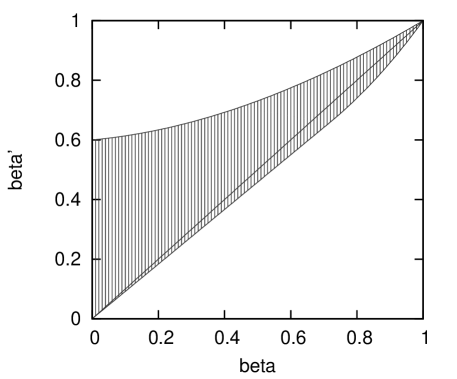
Figure 1: Example of the $\beta^{\prime}$-region (shaded) according to (29) of Proposition 6. The straight line inside the region indicates the value of $\beta$, i.e. the diagonal. Parameters are $\tau=(0.7,0.3)$, $p=(0.6,0.4)$

So in the two-category case we need an estimate of $e_{3,c}$ in order to apply part (iii) of Theorem 1, i.e. we need at least three coders to determine $\beta$ in this case.

As a consequence for the popular two-coder/two-category examples $\beta$ (more precisely the triple $(\beta,\tau,{\bf p})$) is not uniquely determined. In order to determine $\beta$ in such a situation we thus either need to know ${\bf p}$ and use Proposition 4 or ${\bf\tau}$ and apply Proposition 2.

4 Numerical Simulations

The formulae provided by Theorem 1 involve expectation values of coder agreement frequencies. In experiments we typically do not know expectation values but rather observe relative frequencies. Hence we will not obtain the correct values for $\beta$ using the formulae in parts (iii) and (iv) of Theorem 1. Actually, these formulae involve differences of expectation values which are close to 0 for small values of $\beta$, so small statistical fluctuations might lead to large deviations in $\beta$. Thus in order to improve the accuracy we reformulate the problem as a least square optimization problem for the expectation values $e_{1,c}$,$e_{2,c_{1},c_{2}}$ and (if $\#C>2$) $e_{3,c}$, using the formulae for $\beta$ to obtain a start value (augmented by approximations for $\tau$ and $p$ according to (11) and (LABEL:eq:def-e_1) respectively). So find $\beta$, $\tau$, $p$ such that

$$\sum_{c\in C}\left(\beta\tau_{c}+(1-\beta)p_{c}-e_{1,c}\right)^{2}$$

$$+\sum_{c_{1},c_{2}\in C}\left(\beta^{2}\tau_{c}+2\beta(1-\beta)p_{c}\tau_{c}+(1-\beta)^{2}p_{c}^{2}-e_{2,c_{1},c_{2}}\right)^{2}$$

$$+\sum_{c\in C}\left(\beta^{3}\tau_{c}+3\beta^{2}(1-\beta)p_{c}\tau_{c}+3\beta(1-\beta)^{2}p_{c}^{2}\tau_{c}+(1-\beta)^{3}p_{c}^{3}-e_{3,c}\right)^{2}$$

is minimized, subject to the natural constraints.

As we already noted in the introduction the model based approach chosen here allows for simulation runs to investigate the accuracy of this algorithm. The remainder of this section is devoted to such numerical experiments which show the accuracy with varying model parameters. We display the results as inverse empirical distribution functions for a sample of 1000 randomly chosen realizations of the coder model, so the abscissae contain the quantiles and the ordinates the absolute errors (observe the ranges). In the plots the values for the 50 %, 80 %, 90 %, 95 %, 98 %, and 100 % quantiles are highlighted. For every plot we also indicate the other parameters in the caption. The meaning of the parameters is that of the coder model defined in Section 2.

Figure 2: Estimation errors as a function of the true $\beta$ value. Fixed parameters: $N=100$, $m=3$, $R=5$, $\tau=(0.3,0.6,0.1)$, $p=(0.33,0.33,0.34)$

The accuracy in $\beta$ estimation depends on the actual value of $\beta$. As Figure 2 shows, the error decreases with increasing true value of $\beta$. The 98% quantile accuracy ranges from $0.032$ at $\beta_{true}=0.95$ to $0.105$ at $\beta_{true}=0.5$.

According to the coder model a value of $\beta=0.5$ means that only for half of the items the raters could determine the categories with certainty. Note also that if the assumptions of Proposition 3 are satisfied the $S$-value would be as low as 0.25 in this case. Hence the really interesting range for $\beta$ is above 0.5 where the accuracy is higher.

Figure 3: Error of $\beta$ estimate for different true class frequencies. Fixed parameters: $N=100$, $m=3$, $R=5$, $\beta=0.85$, $p=(0.33,0.33,0.34)$

As has been noted before, the definition of $\beta$ does not exhibit the “problem of prevalence”, i.e. its value does not decrease when $\max(\tau)$ approaches $1$. Though the value of $\beta$ is not affected it does affect the accuracy as Figure 3 shows. The 98% quantile accuracy ranges from $0.032$ for $\max(\tau)=\frac{1}{3}$ (the least value of $\max(\tau)$ in this setting) to $0.077$ for $\max(\tau)=0.90$ and $0.22$ for $\max(\tau)=0.95$. In this latter case there are only five of the items not belonging to the prevalent category. Hence statistical fluctuations may blur the distinction of this case from the case $\max(\tau)=1$ where $\beta$ can no longer be determined according to Proposition 1. So this decrease in accuracy is expected.

Figure 4: Error of $\beta$ estimate for different a priori distributions. Fixed parameters: $N=100,m=3,R=5,\beta=0.85,\tau=(0.3,0.6,0.1)$

Contrary to the rather strong impact of $\tau$ on the accuracy, the a priori distribution $p$ does no significantly influence the accuracy as the following Figure 4 shows. Here the 98% quantile errors range from $0.049$ to $0.058$ which may be fully attributed to statistical fluctuations.

Figure 5: Error of $\beta$ estimate for different number of coders. Fixed parameters: $N=100,m=3,\beta=0.85,\tau=(0.3,0.6,0.1),p=(0.33,0.33,0.34)$

Figure 6: Error of $\beta$ estimate for different number of items. Fixed parameters: $m=3,R=5,\beta=0.85,\tau=(0.3,0.6,0.1),p=(0.33,0.33,0.34)$

Finally, since the errors originate from deviations of relative frequencies from the expectation values, the accuracy depends of course moderately on both the number of coders and the number of items. Figure 5 shows the influence of the number of coders on the accuracy. At the 98% quantile level the errors range from $0.03$ (15 coders) to $0.07$ (3 coders). Actually as few as five coders suffice to obtain a reasonably low error of $0.053$.

The impact of the number of items can be seen from Figure 6: With as few as $20$ items one cannot expect more than a rough estimate of beta (error $0.115$ at 98% quantile) with a reasonably low error of $0.054$ when coding 100 items.

References

- [1] Mikel Aickin. Maximum likelihood estimation of agreement in the constant predictive probability model, and its relation to cohen’s kappa. Biometrics, 46(2):pp. 293–302, 1990.
- [2] Ron Artstein and Massimo Poesio. Inter-coder agreement for computational linguistics. Comput. Linguist., 34(4):555–596, December 2008.
- [3] E. M. Bennett, R. Alpert, and A. C. Goldstein. Communications through limited-response questioning. Public Opinion Quarterly, 18(3):303–308, 1954.
- [4] Robert L. Brennan and Dale J. Prediger. Coefficient kappa: Some uses, misuses, and alternatives. Educational and Psychological Measurement, 41(3):687–699, 1981.
- [5] Jacob Cohen. A coefficient of agreement for nominal scales. Educational and Psychological Measurement, 20(1):37–46, 1960.
- [6] Barbara Di Eugenio and Michael Glass. The kappa statistic: A second look. Computational Linguistics, 30(1):95–101, 2004.
- [7] Alvan R. Feinstein and Domenic V. Cicchetti. High agreement but low kappa: I. the problems of two paradoxes. Journal of Clinical Epidemiology, 43(6):543 – 549, 1990.
- [8] Joseph L Fleiss. Measuring nominal scale agreement among many raters. Psychological Bulletin, 76(5):378–382, 1971.
- [9] Kilem Gwet. Kappa statistic is not satisfactory for assessing the extent of agreement between raters. Statistical Methods For Inter-Rater Reliability Assessment, 1(1):1–5, 2002.
- [10] Kilem Li Gwet. Computing inter-rater reliability and its variance in the presence of high agreement. British Journal of Mathematical and Statistical Psychology, 61(1):29–48, 2008.
- [11] Louis M Hsu and Ronald Field. Inter-rater agreement measures: Comments on kappa[n], cohen’s kappa, scott’s pi, and aickin’s alpha. Understanding Statistics, 2(3):205–219, 2003.
- [12] Helena Kraemer. Ramifications of a population model for<i>κ</i> as a coefficient of reliability. Psychometrika, 44:461–472, 1979.
- [13] Klaus Krippendorff. Content Analysis, volume 5 of Sage CommText Series. Sage Publications, Beverly Hills, London, 1980.
- [14] William A Scott. Reliability of content analysis: The case of nominal scale coding. Public Opinion Quarterly, 19(3):321–325, 1955.
- [15] Matthijs Warrens. A formal proof of a paradox associated with cohen’s kappa. Journal of Classification, 27:322–332, 2010.
- [16] Matthijs J. Warrens. A family of multi-rater kappas that can always be increased and decreased by combining categories. Statistical Methodology, 9(3):330 – 340, 2012.
- [17] Rebecca Zwick. Another look at interrater agreement. Psychological Bulletin, 103(3):374 – 378, 1988.