Interference phenomena and long - range proximity effect in clean superconductor – ferromagnet systems

Abstract

We study peculiarities of proximity effect in clean superconductor – ferromagnet structures caused by either spatial or momentum dependence of the exchange field. Even a small modulation of the exchange field along the quasiparticle trajectories is shown to provide a long range contribution to the supercurrent due to the specific interference of particle- and hole- like wave functions. The momentum dependence of the exchange field caused by the spin – orbit interaction results in the long – range superconducting correlations even in the absence of ferromagnetic domain structure and can explain the recent experiments on ferromagnetic nanowires.

The exchange field $h$ in ferromagnetic (F) metals is well known to destroy Cooper pairs resulting, thus, in a strong decay of superconducting (S) correlations in the F material and suppression of Josephson current in SFS junctions (see Refs. Buzdin-rew, ; BergEfVolk-rew, for review). Considering the quantum mechanics of quasiparticle excitations this destructive effect of the exchange field can be viewed as a consequence of a phase difference $\gamma\sim L/\xi_{h}=2Lh/\hbar V_{F}$ gained between the electron- and hole- like parts of the total wave function at the path of the length $L$. Both in the clean and dirty limits the measurable quantities should be calculated as superpositions of fast oscillating contributions $e^{i\gamma}$ from different trajectories and, thus, rapidly vanish with the increasing distance from the SF boundary.

This textbook physical picture appears to be in sharp contrast with a number of recent experiments Robinson ; Khaire ; Sosnin ; Xiao ; Giroud ; Co wire which point to an anomalously large length of decay of superconducting correlations inside the F metal. As we can judge from the observation Co wire of a noticeable supercurrent through a Co nanowire, this decay length can be of the order of half a micrometer which well exceeds typical coherence lengths in ferromagnets both in the clean and dirty limits. In the dirty limit such strong proximity effect can hardly be explained even taking account of long–range triplet correlations BergEfVolk-rew induced by the exchange field inhomogeneity.

Naturally, the inhomogeneity of the field ${\bf h}$ caused by the ferromagnetic domain structure can improve the conditions of Cooper pair survival in the clean limit as well. To suppress the destructive trajectory interference mentioned above the domain structure should cancel the phase gain $\gamma$ for a certain group of quasiparticle trajectories. A simple example of such phase gain compensation can be realized in a clean junction consisting of two F layers with opposite orientations of magnetic moment blanter ; pajovic . On the other hand in the diffusive limit this compensation effect vanishes crouzy . Note, that the exchange field inhomogeneity along the quasiclassical trajectory experiencing multiple reflections from the ferromagnet surface can appear even in the absence of the spatial domain structure. Indeed, the exchange field acting on band electrons in a solid with a finite spin – orbit interaction should obviously depend on the quasiparticle momentum shekhter : ${\bf h}={\bf h}({\bf k})$. The normal quasiparticle reflection is accompanied, of course, by the change in the momentum direction, and, thus, by the change in the exchange field. The momentum dependent ${\bf h}$ field can strongly affect the phase gain $\gamma$ along the trajectories even in the F sample prepared in a single domain state (as it has been done in experiments with Co nanowires Co wire ).

The goal of this paper is to show that in the clean limit there exists a possibility to cancel the particle – hole phase difference for a large group of quasiclassical trajectories due to either spatial or momentum dependence of the exchange field. Such set of trajectories provides a long–range contribution to the Josephson current through a ferromagnetic system which decays at the length scale characteristic for a nonmagnetic metal. We consider two generic examples which illustrate the above scenario of a long–range proximity effect: (i) Josephson transport through a pair of ferromagnetic layers with a stepwise exchange field distribution; (ii) Josephson transport through a nanowire with a specular electron reflection at the surface and exchange field varying with the changing quasiparticle momentum. See Supplemental Material at [URL will be inserted by publisher] for details of calculations.

Josephson transport through a ferromagnetic bilayer.

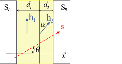
Figure 1: (Color online) Josephson junction containing two ferromagnetic layers. Linear quasiparticle trajectory is shown by the red dashed line.

Let us start from the simplest model illustrating the origin of the quasiparticle interference suppression: Josephson junction containing two ferromagnetic layers of the thicknesses $d_{1}$ and $d_{2}$, respectively (see Fig.1). Here we consider the limit of short junction $d_{1}+d_{2}\ll\xi_{s}$, where $\xi_{s}$ is the superconducting coherence length. The exchange fields ${\bf h}_{1}$ and ${\bf h}_{2}$ in the layers are rotated at the angle $\alpha$. Following the quasiclassical procedure considered in Ref. Buzdin-prb11, we find the current – phase relation:

$$I=\sum\limits_{n}I_{n}=\sum\limits_{n}a_{n}\sin n\varphi\frac{\langle({\bf n},{\bf n}_{F})\cos n\gamma\rangle}{\langle({\bf n},{\bf n}_{F})\rangle}\ ,$$ (1)

where ${\bf n}$ is the unit vector normal to the junction plane, ${\bf n}_{F}$ is the unit vector along the trajectory, and $a_{n}$ are the coefficients of the Fourier expansion for the current – phase relation $I_{SNS}(\varphi)$ for zero exchange field, i.e., for superconductor – normal metal junction of the same geometry. The angular brackets denote the averaging over different quasiclassical trajectories. The first two coefficients in this expansion take the form:

$$a_{n}=\frac{4eT}{\hbar}N(-1)^{n-1}\sum_{m=0}^{\infty}\left(\mu_{m}-\sqrt{\mu_{m}^{2}-1}\right)^{n},\;n=1,2,\\$$ (2)

where $\mu_{m}=2\pi^{2}T^{2}(2m+1)^{2}/\Delta_{0}^{2}+1$, $\Delta_{0}$ is the temperature dependent superconducting gap, $N=s_{0}^{-1}\int ds\int d{\bf n}_{F}(\mathbf{n}_{F},\mathbf{n})$, $s_{0}^{-1}=k_{F}/2\pi$ ($s_{0}^{-1}=(k_{F}/2\pi)^{2}$) for 2D (3D) junctions, and the integral $\int\ldots ds$ is taken over the junction cross–section. The factor $N$ is determined by the number of transverse modes in the junction: $N\sim S/s_{0}$, where $S$ is the junction cross–section area.

The phase $\gamma$ can be found from the singlet part of the anomalous quasiclassical Green function:

$$f_{s}(s=s_{R})=\cos\gamma$$

taken at the right superconducting electrode. Here we use a standard parametrization Champel $f=f_{s}+\textbf{f}_{t}\hat{\sigma}$, where $\hat{\sigma}$ is a Pauli matrix vector in the spin space. The functions $f_{s}$, $\textbf{f}_{t}$ satisfy the linearized Eilenberger equations written for zero Matsubara frequencies

$$-i\hbar V_{F}\partial_{s}f_{s}+2\textbf{h}\textbf{f}_{t}=0\ ,\quad-i\hbar V_{F}\partial_{s}\textbf{f}_{t}+2f_{s}\textbf{h}=0\ ,$$ (3)

and the conditions $f_{s}(s=s_{L})=1$, $\textbf{f}_{t}(s=s_{L})=0$ at the left superconducting electrode. Solving the above equations for the particular bilayer geometry we find:

$$\cos\gamma=\cos^{2}\frac{\alpha}{2}\,\cos\left(\frac{d_{1}+d_{2}}{\xi_{h}\cos\theta}\right)+\sin^{2}\frac{\alpha}{2}\,\cos\left(\frac{d_{1}-d_{2}}{\xi_{h}\cos\theta}\right)\ ,$$ (4)

where $\cos\theta=({\bf n},{\bf n}_{F})$. This expression allows us to write the first harmonic in the current – phase relation in the form:

$$I_{1}=\left[\cos^{2}\frac{\alpha}{2}\,I_{c1}\left(\frac{d_{1}+d_{2}}{\xi_{h}}\right)+\sin^{2}\frac{\alpha}{2}\,I_{c1}\left(\frac{d_{1}-d_{2}}{\xi_{h}}\right)\right]\sin\varphi\ ,$$ (5)

where $I_{c1}(d/\xi_{h})$ is the critical current of the first harmonic in a SFS junction with a homogeneous exchange field $h$. The interference effects discussed in introduction result in the power decay of the critical current $I_{c1}$ vs the F layer thickness $d$: $I_{c1}\propto d^{-1/2}$ for a 2D junction 2D and $I_{c1}\propto d^{-1}$ for a 3D junction 3D . Taking symmetric case $d_{1}=d_{2}$ we immediately get a long–range contribution to the Josephson current

$$\delta I_{c1}=\sin^{2}\frac{\alpha}{2}\,I_{c1}\left(0\right)\sin\varphi\ ,$$ (6)

which does not decay with the increasing distance between the S electrodes. It is important to note that this contribution does not vanish for an arbitrary nonzero angle between the magnetic moments in the F layers.

Long–range behavior can be observed for a second harmonic in the current – phase relation as well. Indeed, calculating the average $\langle({\bf n},{\bf n}_{F})\cos 2\gamma\rangle$ we find a nonvanishing long–range supercurrent contribution even for $d_{1}\neq d_{2}$:

$$\delta I_{c2}=\frac{a_{2}\sin^{2}\alpha}{2}\sin 2\varphi\ .$$ (7)

Note, that the emergence of long–range proximity effect for high harmonics in Josephson relation is in a good agreement with recent theoretical findings in Refs. trifunovic1, ; trifunovic2, .

Josephson current through a ferromagnetic wire. We now proceed with the consideration of a more complicated example of the interference phase suppression in a ferromagnetic wire where the quasiclassical trajectories of electrons and holes experience multiple specular reflections from the wire surface (see Fig. 2a). The particular geometry shown in Fig. 2a can be considered as a rough model for experiments on Co nanowires Co wire . For simplicity we restrict ourselves to the case of a 2D junction.

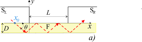
Figure 2: (Color online) Josephson transport through a nanowire in the overlap (a) and edge (b) geometries. The quasiparticle trajectories are shown by the red dashed lines.

Taking account of the spin-orbit interaction inside the ferromagnet we obtaine the exchange part of the effective Hamiltonian for the band electrons depending on the quasi-momentum ($\mathbf{k}$) orientation:

$$\hat{H}_{ex}=\sum\limits_{ij}\beta_{ij}(\mathbf{k})h_{0i}\sigma_{j}=\mathbf{h}(\mathbf{k})\hat{\sigma}\,,$$

where $\mathbf{h}_{0}$ is a pseudo vector determined by the ferromagnetic moment. Assuming the absence of the system anisotropy described by a polar vector we find the simplest form of the resulting exchange field: $\mathbf{h}=\mathbf{h}_{0}+\beta_{so}k_{F}^{-2}(\mathbf{h}_{0},\mathbf{k})\mathbf{k}$, where $\beta_{so}$ is a constant determined by the spin – orbit interaction, and $k_{F}$ is the Fermi momentum.

The exchange field along the quasiparticle trajectory experiencing the reflection at the wire surface should change its direction. Thus, we obtain the problem described by Eqs. (3) with a periodic exchange field along the trajectory characterized by a given angle $\theta$ and a certain starting point at the superconductor surface. The same equations for each trajectory can be of course derived for a periodic domain structure. Let us consider first the problem of calculating the band spectrum $\epsilon(k)$ in the field $\mathbf{h}$ varying with the period $2D/\sin\theta$:

$$-i\hbar V_{F}\partial_{s}f_{s}+2\textbf{h}\textbf{f}_{t}=\epsilon(k)f_{s}\,,$$ (8)

$$-i\hbar V_{F}\partial_{s}\textbf{f}_{t}+2f_{s}\textbf{h}=\epsilon(k)\textbf{f}_{t}\,.$$ (9)

The solution can be written in the Bloch form:

$$\left(f_{s}\atop\textbf{f}_{t}\right)=e^{iks}\left(f_{sk}\atop\textbf{f}_{tk}\right)\ ,$$

where $f_{sk}(s+2D/\sin\theta)=f_{sk}(s)$ and $\textbf{f}_{tk}(s+2D/\sin\theta)=\textbf{f}_{tk}(s)$. One can see that provided this solution corresponds to the energy branch $\epsilon_{\sigma}(k)$ there exist another solution $(f_{s}^{*},-\textbf{f}_{t}^{*})$ corresponding to the energy $-\epsilon_{\sigma}(k)$. On the other hand the latter solution corresponds also to the energy $\epsilon_{\tilde{\sigma}}(-k)$ and, thus, we obtain the following symmetry property of the band spectrum: $\epsilon_{\tilde{\sigma}}(-k)=-\epsilon_{\sigma}(k)$, where the indices $\sigma$ and $\tilde{\sigma}$ denote different branch numbers. The full set of energy branches can be split in such pairs provided the number of branches is even. For an odd number of branches there is always one branch which does not have a partner. For this branch we obtain $\epsilon_{\sigma}(-k)=-\epsilon_{\sigma}(k)$ and, thus, this spectrum branch crosses the zero energy level at $k=0$: $\epsilon_{\sigma}(0)=0$. The corresponding phase gain $\gamma$ appears to vanish for trajectories containing an integer number of periods shown in Fig. 2a and, therefore, the solution with $k=0$ and $\epsilon=0$ provides a long–range contribution to the supercurrent.

For the sake of definiteness we choose the field $\mathbf{h}_{0}$ to be directed along the wire axis $x$ and obtain the exchange field in the form: $\mathbf{h}=\mathbf{x}_{0}h_{x}+\mathbf{y}_{0}h_{y}(s)$, where $h_{x}(\theta)\simeq h_{0}$ is constant along the trajectory and $h_{y}(s)$ is a periodic function with zero average. In the interval $-D/\sin\theta<s<D/\sin\theta$ the $h_{y}$ field component is defined by the expression $h_{y}=\beta_{so}h_{0}\sin\theta\cos\theta\,{\rm sign}\,s$. Introducing the Fourier expansions

$$h_{y}=\sum\limits_{q}H_{q}\mathrm{e}^{iqs}\ ,\,\,\,\,\,H_{q}=-i\tilde{h}\frac{2\sin\theta}{Dq}\,,$$

$$f_{s,tx,ty}=\mathrm{e}^{iks}\sum\limits_{q}F_{s,x,y}(k+q)\mathrm{e}^{iqs}\,,$$

we rewrite the Eqs. (8) and (9) in the form:

$$(\hbar V_{F}(k+q)-\epsilon)F_{s}(k+q)+2h_{x}F_{x}(k+q)$$

$$\qquad\quad+2\sum\limits_{\tilde{q}}H_{q-\tilde{q}}F_{y}(k+\tilde{q})=0\,,$$ (10)

$$(\hbar V_{F}(k+q)-\epsilon)F_{x}(k+q)+2h_{x}F_{s}(k+q)=0\,,\qquad$$ (11)

$$(\hbar V_{F}(k+q)-\epsilon)F_{y}(k+q)$$

$$\qquad\quad+2\sum\limits_{\tilde{q}}H_{q-\tilde{q}}F_{s}(k+\tilde{q})=0\,.$$ (12)

Here $q,\tilde{q}=q_{m}=\pi(2m+1)\sin\theta/D$, $m$ is an integer, and $\tilde{h}=\beta_{so}h_{0}\sin\theta\cos\theta$.

To get the solution for a small periodic field $h_{y}$ we use a perturbative approach similar to the nearly free electron approximation in the band theory of solids and restrict the number of interacting Fourier harmonics in the expansions. For this purpose it is instructive to consider the limit of zero periodic potential $h_{y}$ and separate three types of solutions: (i) the solution $(F_{s},F_{x},F_{y})=(0,0,1)\delta_{q-p}$ corresponding to the energy $\epsilon_{0}=\hbar V_{F}(k+p)$ (ii) the solutions $(F_{s},F_{x},F_{y})=(1,\pm 1,0)\delta_{q-p_{\pm}}$ corresponding to the energies $\epsilon_{\pm}=\hbar V_{F}(k+p_{\pm})\pm 2h_{x}$. Here $p$ and $p_{\pm}$ are arbitrary reciprocal lattice vectors. The above modes should strongly interact provided the resonant condition $\epsilon_{0}=\epsilon_{+}=\epsilon_{-}$ is fulfilled. Such resonance is possible for the case when the value $2h_{x}/\hbar V_{F}$ equals to a certain reciprocal lattice vector $q_{m}$. Close to such Bragg – type resonance we see that the dominant harmonics correspond to the following choice of reciprocal lattice vectors: $p=0$, $p_{\pm}=\mp q_{m}$. Writing the solution as a superposition of these three harmonics we find renormalized spectral branches $\epsilon_{0}=\hbar V_{F}k$, $\epsilon_{\pm}=\hbar V_{F}k\pm\sqrt{(\hbar V_{F}q_{m}-2h_{x})^{2}+8|H_{q_{m}}|^{2}}$ and corresponding eigenfunctions. Applying now the boundary conditions at $s=0$ for the superposition of the above eigenfunctions we find the amplitude of the singlet component corresponding to the energy branch $\epsilon_{0}$ and $k=0$:

$$f_{sm}=\frac{8|H_{q_{m}}|^{2}\cos(q_{m}s)}{(\hbar V_{F}q_{m}-2h_{x})^{2}+8|H_{q_{m}}|^{2}}\ .$$

At the surface of a right superconducting electrode we should take the coordinate $s$ to be equal to the integer number of periods. We also need to sum up the above resonant expressions over all Fourier harmonics of the periodic potential:

$$f_{s}(s=s_{R})=\sum\limits_{m=0}^{\infty}\frac{8|H_{q_{m}}|^{2}}{(\hbar V_{F}q_{m}-2h_{x})^{2}+8|H_{q_{m}}|^{2}}\ .$$

The precision of such resonant – type expression has been also confirmed by the numerical solution of the Eqs. (8) and (9) carried out using the transfer matrix method. Note, that we omit here the contribution from the solutions corresponding to the branches $\epsilon_{\pm}$: these functions correspond to a nonzero quasimomentum and, thus, should gain a finite phase factor along the trajectory length. During averaging over different trajectories this phase factor causes the suppression of the resulting supercurrent contribution with the increasing wire length $L$.

The starting point of the trajectory varies in the interval $\Delta x=2D/\tan\theta$ and, as a consequence, the long – range first harmonic in current – phase relation takes the form:

$$I_{1}=a_{1}\sin\varphi\int\limits_{0}^{\pi/2}d\theta\cos\theta f_{s}(s_{R})\,.$$

Assuming the resonances to be rather narrow we approximate them by the delta – functions and obtain:

$$I_{1}=a_{1}\sin\varphi\sum\limits_{m}\frac{\sqrt{2}\pi\hbar V_{F}\tilde{h}(\theta_{m})}{h_{x}^{2}D}\sin^{2}\theta_{m}\,.$$

where $\sin\theta_{m}=2h_{x}D/\pi\hbar V_{F}(2m+1)$. In the limit $D\gg\hbar V_{F}/2h_{x}$ one can replace the sum over $m$ by the integral:

$$I_{1}\simeq a_{1}\sqrt{2}\int\limits_{0}^{\pi/2}d\theta\frac{\tilde{h}(\theta)}{h_{x}(\theta)}\cos\theta\sin\varphi\simeq a_{1}\frac{\sqrt{2}}{3}\beta_{s0}\sin\varphi\ .$$

Certainly, the above long–range effect in the first harmonic is rather sensitive to the system geometry: taking, e.g., the system sketched in Fig. 2b we will not obtain the full cancellation of the phase $\gamma$ because the trajectories in this case do not contain integer number of exchange field modulation periods. However, similarly to the case of bilayer the long–range effect is still possible for higher harmonics. We apply the above perturbative procedure for the calculation of the full $f_{s}$ function for the geometry shown in Fig. 2b. The second harmonic in the current–phase relation reads

$$I_{2}=a_{2}\sin 2\varphi\ \int\limits_{0}^{\pi/2}d\theta\cos\theta\left(\,2\langle f_{s}^{2}(s_{R})\rangle_{y_{0}}-1\,\right)\,,$$ (13)

where $\langle\ldots\rangle_{y_{0}}=(1/D)\int_{0}^{D}\ldots dy_{0}$ denotes averaging over the starting point of the trajectory $y_{0}$ (see Fig. 2b). Keeping only the terms linear in the small $|H_{q_{m}}|$ amplitude we get the following expression for the long–range part of the second harmonic $I_{2}$:

$$I_{2}=a_{2}\sin 2\varphi\sum\limits_{m}\frac{\sqrt{2}\pi\hbar V_{F}\tilde{h}(\theta_{m})}{h_{x}^{2}D}\sin^{2}\theta_{m}\simeq a_{2}\frac{\sqrt{2}}{3}\beta_{s0}\sin 2\varphi.$$

We emphasize that the second harmonic of Josephson current in both above examples is negative because of the condition $a_{2}<0$.

Note that the absence of the decay of the single-channel critical current was pointed out in Ref. buzdin, as a possible source of the long-ranged proximity effect in Co nanowires. However the averaging of the phase gain for different modes strongly decreases the critical current. In contrast the results presented in this Letter demonstrate that in the ballistic regime the spin-orbit interaction generates the non-collinear exchange field which produces the long – range Josephson current. This conclusion is always true for the second harmonic in the current – phase relation and for some geometries it may be also valid for the first harmonic. Therefore our findings provide a natural explanation of the recent experiments with Co nanowire Co wire . To discriminate between two proposed mechanisms of the long ranged effect, the studies of higher harmonics in Josephson current-phase relations could be of major importance. Also it should be interesting to verify on experiment the predicted simple angular dependence (6) of the critical current in S/F/S junctions with composite interlayer.

- (1) A. I. Buzdin, Rev. Mod. Phys., 77, 935 (2005).
- (2) F. S. Bergeret, A. F. Volkov, and K. B. Efetov, Rev. Mod. Phys., 77, 1321 (2005).
- (3) J. W. A. Robinson, J. D. S. Witt, and M. G. Blamire, Science 329. 59 (2010).
- (4) T. S. Khaire, M. A. Khasawneh, W. P. Pratt, Jr., and N. O. Birge, Phys. Rev. Lett. 104, 137002 (2010).
- (5) I. Sosnin, H. Cho, and V. T. Petrashov, A. F. Volkov, Phys. Rev. Lett. 96, 157002 (2006).
- (6) R. S. Keizer, S. T. B. Goennenwein, T. M. Klapwijk, G. Miao, G. Xiao, and A. Gupta, Nature, 439, 825 (2006).
- (7) M. Giroud, H. Courtois, K. Hasselbach, D. Mailly, and B. Pannetier, Phys. Rev. B 58, R11872 (1998).
- (8) Jian Wang, Meenakshi Singh, Mingliang Tian, Nitesh Kumar, Bangzhi Liu, Chuntai Shi, J. K. Jain, Nitin Samarth, T. E. Mallouk & M. H. W. Chan, Nature Physics, 6, 389 (2010).
- (9) Ya. M. Blanter and F. W. J. Hekking, Phys. Rev. B 69, 024525 (2004).
- (10) Z. Pajovic, M. Bozovic, Z. Radovic, J. Cayssol and A. Buzdin, Phys. Rev. B 74, 184509 (2006).
- (11) B. Crouzy, S. Tollis, and D. A. Ivanov, Phys. Rev. B 75, 054503 (2007).
- (12) A. Kadigrobov, Z. Ivanov, T. Claeson, R. I. Shekhter, and M. Jonson, Europhys. Lett. 67, 948 (2004).
- (13) A. I. Buzdin, A. S. Melnikov, and N. G. Pugach, Phys. Rev. B 83, 144515 (2011).
- (14) T. Champel, T. Löfwander, and M. Eschrig, Phys. Rev. Lett. 100, 077003 (2008). Thierry Champel1,2, Tomas Lo”fwander1,3, and Matthias Eschrig
- (15) F. Konschelle, J. Cayssol, and A. I. Buzdin, Phys. Rev. B 78, 134505 (2008).
- (16) A. I. Buzdin, L. N. Bulaevskii, and S. V. Panyukov, JETP Lett. 35, 178 (1982) [Pis’ma Zh. Eksp. Teor. Fiz. 35, 147 (1982)].
- (17) L. Trifunovic, Phys. Rev. Lett. 107, 047001 (2011).
- (18) L. Trifunovic, Z. Popovic, and Z. Radovic, Pys. Rev. B 84, 064511 (2011).
- (19) F. Konschelle, J. Cayssol, and A. Buzdin, Phys. Rev. B 82, 180509 (2010).