Microscopic theory for the Doppler velocimetry of spin propagation in semiconductor quantum wells

Abstract

We provide a microscopic theory for the Doppler velocimetry of spin propagation in the presence of spatial inhomogeneity, driving electric field and the spin orbit coupling in semiconductor quantum wells in a wide range of temperature regime based on the kinetic spin Bloch equation. It is analytically shown that under an applied electric field, the spin density wave gains a time-dependent phase shift $\phi(t)$. Without the spin-orbit coupling, the phase shift increases linearly with time and is equivalent to a normal Doppler shift in optical measurements. Due to the joint effect of spin-orbit coupling and the applied electric field, the phase shift behaves differently at the early and the later stages. At the early stage, the phase shifts are the same with or without the spin-orbit coupling. While at the later stage, the phase shift deviates from the normal Doppler one when the spin-orbit coupling is present. The crossover time from the early normal Doppler behavior to the anomalous one at the later stage is inversely proportional to the spin diffusion coefficient, wave vector of the spin density wave and the spin-orbit coupling strength. In the high temperature regime, the crossover time becomes large as a result of the decreased spin diffusion coefficient. The analytical results capture all the quantitative features of the experimental results, while the full numerical calculations agree quantitatively well with the experimental data obtained from the Doppler velocimetry of spin propagation [Yang et al., Nat. Phys. 8, 153 (2012)]. We further predict that the coherent spin precession, originally thought to be broken down at high temperature, is robust up to the room temperature for narrow quantum wells. We point out that one has to carry out the experiments longer to see the effect of the coherent spin precession at higher temperature due to the larger crossover time.

I Introduction

Understanding the spin transport phenomena is one of the most important issues in the fast developing field of spintronicsAwschalom et al. (2002); Žutić et al. (2004); Fabian et al. (2007); Dyakonov (2008); Wu et al. (2010); Tsymbal and Žutić (2011) since it is crucial to the realization of the spintronic devices, such as spin-field-effect transistor.Datta and Das (1990); Appelbaum and Monsma (2007); Appelbaum et al. (2007); Koo et al. (2009); Wunderlich et al. (2010) In the proposed Datta-Das transistor,Datta and Das (1990) the “on” and “off” states, distinguished by a $\pi$-phase difference in the spin precession mode, are switched by the gate voltage which controls the coherent spin precession (CSP) of the passing carriers via the Rashba spin-orbit coupling (SOC)Bychkov and Rashba (1984) acting as an effective magnetic field. To implement such devices, it is required that one is able to control and maintain spin polarization over a long enough distance, preferably at room temperature.

Experimentally, the real space spin transport in semiconductor is studied by using magneto-optic imaging,Crooker and Smith (2005); Beck et al. (2006) or through conductance/current modulation.Koo et al. (2009); Wunderlich et al. (2010) An important development in the quantitative study of the spin transport is carried out by using spin transient grating spectroscopy.Yang et al. (2012); Cameron et al. (1996); Weber et al. (2005); Carter et al. (2006); Weber et al. (2007); Yang et al. (2010) In these experiments, a spin density wave (SDW) with initial spin polarization $S_{z}(x,0)=S_{0}\cos(qx)$ is created by two orthogonal linear polarized light beams at time $t=0$, where $q$ is the wave vector of the SDW and $x$ is the position. Under the influence of an applied in-plane electric field and the SOC, SDW picks up a phase and evolves into $S_{z}(x,t)=S^{0}_{z}(q,t)\cos(qx-\phi(t))$. By optically monitoring the temporal evolution of the amplitude $S^{0}_{z}(q,t)$, one obtains the spin diffusion coefficient and relaxation rate.Cameron et al. (1996); Weber et al. (2005); Carter et al. (2006); Weber et al. (2007); Yang et al. (2010, 2012); Weng et al. (2008) Very recently, the spin drifting and CSP were studied by the Doppler velocimetry which monitors the phase shift $\phi(t)$.Yang et al. (2011, 2012) For pure spin drift without spin precession, the phase shift is simply $\phi(t)=qv_{d}t$, where $v_{d}$ stands for the drift velocity. The linear increase of phase shift with time is equivalent to a Doppler shift $\Delta\omega=v_{d}q$. When both the CSP and drifting are present, the phase shift deviates from this simple relation and behaves anomalously. In Ref. [Yang et al., 2012], Yang et al. reported that at low temperature ($T=30$ K), $\phi(t)$ deviates strongly from the simple relation of $qv_{d}t$ and clearly shows the anomalous behavior caused by the CSP. However, once the temperature rises to 150 K, the anomalous behavior of the phase shift disappears in the time frame of the observation. It was then concluded that CSP breaks down at high temperature, although the mechanism of the disappearance of CSP is not clear.Yang et al. (2012) The disappearance of CSP at high temperature was claimed to be in consistence with the previous experimental results in the prototypes of Datta-Das transistors.Koo et al. (2009)

The temporal evolution of the SDW contains all of the important information of spin transport, such as spin diffusion coefficient, spin mobility and CSP. The transient spin grating spectroscopy together with the Doppler velocimetry therefore enable one to quantitatively study the spin transport in semiconductors. However, the dynamics of SDW is quite complex when spatial inhomogeneity, applied electric field as well as the SOC are present. To correctly extract the information from the experimental data, a thorough understanding of spin transport is in demand. Without the electric field, the amplitude $S^{0}_{z}(q,t)$ decays biexponentially when the SDW diffuses along the $[1\bar{1}0]$ crystal axis in (001) GaAs quantum wells (QWs) as spin rotates along the net effective magnetic field due to the SOC and diffusion.Weber et al. (2005); Weng et al. (2008); Lüffe et al. (2011) Based on the kinetic spin Bloch equation (KSBE) approach,Weng et al. (2004); Wu et al. (2010) it is shown that the information about spin diffusion coefficient, CSP and spin relaxation can be extracted from the wave-vector dependence of the two decay rates.Weng et al. (2008) In this paper we will further extend the theory to include the electric field and show, both analytically and numerically, that the theoretical and experimental results agree well with each other. We will demonstrate that the CSP is robust even in high temperature regime for narrow QWs and point out that to observe the effect of the CSP at high temperature, one has to carry out the observation for a longer time than the case at low temperature.

II Analytical results of the evolution of the SDW

As will be shown later, the SDW transporting along the $[1\bar{1}0]$ crystal axis with the wave vector $q$ in a $(001)$ GaAs QW evolves as

$$S_{z}(x,t) = S_{z}(q,0)\exp[-(Dq^{2}+1/\tau_{s})t]/2$$ (1)

$$\mbox{ }\times\Bigl{\{}e^{-2Dqq_{0}t}\cos[qx-v_{d}(q+q^{\prime}_{0})t]$$

$$\mbox{ }+e^{2Dqq_{0}t}\cos[qx-v_{d}(q-q^{\prime}_{0})t]\Bigr{\}}\;,$$

when the SOC is weak enough. Here $D$, $\tau_{s}$ and $v_{d}$ are the spin diffusion coefficient, spin relaxation time of the SDW and the drift velocity under the electric field $E$, respectively. $q_{0}=m^{\ast}(\hat{\beta}+\alpha)$ and $q^{\prime}_{0}=m^{\ast}(\hat{\beta}^{\prime}+\alpha)$ with $m^{\ast}$ representing the effective mass, $\alpha$ being the Rashba coefficientBychkov and Rashba (1984) and $\hat{\beta}$, $\hat{\beta}^{\prime}$ both standing for the coefficients of the linear Dresselhaus termD’yakonov and Perel’ (1971a) with corrections from the cubic Dresselhaus terms.Weng et al. (2008) Without the applied electric field, $v_{d}=0$ and the amplitude of the SDW decays biexponentially with fast and slow rates $Dq^{2}+1/\tau_{s}\pm 2Dqq_{0}$.Weber et al. (2005); Weng et al. (2008) When there is an applied electric field but without the CSP ($q_{0}=q_{0}^{\prime}=0$), the SDW decays exponentially and gains a phase shift which changes linearly with time with a slope $qv_{d}$, which is equivalent to a normal Doppler shift in experiments. With the CSP, the situation is more complex. For small time $t\ll 1/(4D|qq_{0}|)$, the fast and the slow modes share the same weights. Therefore the phase shift of the SDW reads

$$\phi(t)\simeq[v_{d}(q+q_{0}^{\prime})t+v_{d}(q-q_{0}^{\prime})t]/2=v_{d}qt\;.$$ (2)

Nevertheless, for large time $t\gg 1/(4D|qq_{0}|)$, the slow mode dominates and the phase shift becomes

$$\phi(t)\simeq v_{d}(q-q^{\prime}_{0})t\;.$$ (3)

That is, in the presence of the CSP, the phase shift first changes linearly with a slope $qv_{d}$, same as the normal Doppler one without the CSP. After some time, the slope deviates from the normal one and reduces to $v_{d}(q-q^{\prime}_{0})$. The sign of the slope reverses when $q<q^{\prime}_{0}$. In the special case of $q=q_{0}^{\prime}$, the phase approaches a stationary value at large time. The crossover time of $\phi(t)$ from the normal Doppler behavior in the early stage to the anomalous one at the later stage is about $t_{c}\sim 1/(4D|qq_{0}|)$. In the case of small diffusion coefficient, wave vector of SDW or the SOC, this crossover time can be larger.

Equation (1) captures all of the qualitative features of the experimental resultsYang et al. (2012) at low temperature, from the two modes in the temporal evolution of SDW when $E=0$ (hence $v_{d}=0$), to the details of how the phase changes with time and wave vector when $E\not=0$. Specifically, the temporal evolution of the phase can be divided into two stages. In the early stage, the phase increases with time with a steeper slope. The slope becomes flatter in the later stage, or even reverses its sign for small wave vectors. The larger the wave vector is, the quicker the phase behavior changes from the early stage to the later stage. All these features qualitatively agree with Eq. (1).

As a result of the increasing electron-phonon scattering and spin Coulomb drag,D’Amico and Vignale (2000); Weber et al. (2005); Takahashi et al. (2008); Badalyan et al. (2008) the spin diffusion coefficient $D$ decreases with the increase of temperature. It is therefore expected that at high temperature the crossover time is larger than that at low temperature. With the correction of the cubic Dresselhaus term, $q_{0}$ also reduces as the temperature rises and the crossover time is further prolonged. If the contribution from the cubic Dresselhaus term is so large that $q_{0}$ approaches zero, then the CSP breaks down completely at high temperature. In the recent experiments, the CSP is thought to be broken down at high temperature based on the lack of the clear anomalous behavior in the phase shift from the observation in a limited time regime. The cubic Dresselhaus term is speculated to be the main cause for the breaking down.Yang et al. (2012) However, this is highly unlikely because $q_{0}$ at low temperature only differs by a few percents from the one at high temperature for the narrow QW used in the experiments. It should be pointed out that, since the behaviors of phase in the early stage are the same with or without the CSP, one should be cautious in determining the existence of such CSP from the experimental data in limited time regime, especially when the crossover time $t_{c}$ is large. In our opinion, purely from the existing experiments, it is inconclusive to determine whether the CSP survives or not at high temperature.

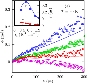
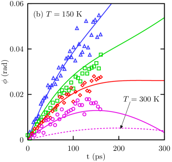
Figure 1: (Color online) Phase shifts of drifting spin grating under an applied electric field of $E=2$ V/cm for different wave vector at (a) $T=30$ K and (b) $T=150$ K. Blue Curve/Triangle: $q=1.07$ cm^-1; Green Curve/Square: $q=0.81$ cm^-1; Red Curve/Diamond: $q=0.59$ cm^-1; Purple Curve/Circle: $q=0.34$ cm^-1, respectively. Inset of (a): Fitting of spin relaxation times $\tau_{+}$ (Red Curve/Circle) and $\tau_{-}$ (Blue Curve/Triangle) at $T=30$ K. The dashed purple curve in (b) is the phase shift for $q=0.34$ cm^-1 at $T=300$ K. All the curves in the figures are from theoretical calculation whereas the symbols are the experimental data from Ref. [Yang et al., 2012].

To derive the solution [Eq. (1)] and to determine if the CSP is stable at high temperature, we turn to the full KSBEs for the spin transport in a (001) GaAs QW grown along the $z$-axisWu et al. (2010); Tsymbal and Žutić (2011); Weng et al. (2004)

$${\partial\rho_{\mathbf{k}}(x,t)\over\partial t}=-eE(x){\partial\rho_{\mathbf{k}}(x,t)\over\partial k_{x}}+{k_{x}\over m^{\ast}}{\partial\rho_{\mathbf{k}}(x,t)\over\partial x}$$

$$\mbox{ }+i[\mathbf{h}_{tot}(\mathbf{k}))\cdot\mbox{\boldmath$\sigma$}/2,\rho_{\mathbf{k}}(x,t)]+\left.{\partial\rho_{\mathbf{k}}(x,t)\over\partial t}\right|_{\mathtt{s}}.$$ (4)

Here we assume that the transport direction is along the $x$-axis. $\rho_{\mathbf{k}}(x,t)$ are the density matrices of electron with momentum $\mathbf{k}=(k_{x},k_{y})=(k\cos\phi,k\sin\phi)$ at position $x$. The right hand side of Eq. (4) describes the drift of electrons driven by the electric field $E(x)$, diffusion caused by the spatial inhomogeneity, spin precession around the total magnetic field ${\bf h}_{tot}({\bf k})$ and all the scattering, respectively. The total magnetic field is composed of the external magnetic field $\mathbf{B}$ in the Voigt configuration, the effective magnetic field $\mathbf{h}(\mathbf{k})$ due to the SOC as well as the one from the Hartree-Fock term of the electron-electron Coulomb interaction. The expressions for the Hartree-Fock and the scattering terms are given in detail in Refs. [Weng et al., 2004b; Wu et al., 2010]. $\mathbf{h}(\mathbf{k})$ contains the Dresselhaus and the Rashba terms:D’yakonov and Perel’ (1971a); Bychkov and Rashba (1984)

$$\mathbf{h}(\mathbf{k}) = \beta(-k_{x}\cos 2\theta+k_{y}\sin 2\theta,k_{x}\sin 2\theta+k_{y}\cos 2\theta,0)$$ (5)

$$+\gamma({k_{x}^{2}-k_{y}^{2}\over 2}\sin 2\theta+k_{x}k_{y}\cos 2\theta)(k_{y},-k_{x},0)$$

$$+\alpha(k_{y},-k_{x},0)\ ,$$

where $\theta$ is the angle between $x$-axis (the spin injection/diffusion direction) and the $(100)$ crystal axis.Cheng et al. (2007); Weng et al. (2008) $\beta=\gamma\pi^{2}/a^{2}$ with $\gamma$ being the Dresselhaus coefficient.D’yakonov and Perel’ (1971a) $\alpha$ represents the Rashba parameter which depends on the electric field along the growth direction of the QW. Note that we have included the corrections from the cubic Dresselhaus term.

By expanding the density matrix $\rho_{\bf k}(x,t)=\sum_{l}\rho_{l}(x,k,t)e^{il\phi}$, the KSBEs can be written as a series of coupled equations for $\rho_{l}(x,k,t)$. By neglecting the Hatree-Fock term and the inelastic scattering and using the fact that the spin density is ${\bf S}(x,t)=\sum_{\bf k}\mathtt{Tr}\{\mbox{\boldmath$\sigma$\unboldmath}\rho_{\bf k}(x,t)\}=\int_{0}^{\infty}\mathtt{Tr}[\mbox{\boldmath$\sigma$\unboldmath}\rho_{0}(x,k,t)]kdk/2\pi$, one finds that, to the leading order, under a uniform applied electric field $E$ the spin density obeys the following equation

$${\partial{\bf S}\over\partial t}=D{\partial^{2}{\bf S}\over\partial x^{2}}+v_{d}{\partial{\bf S}\over\partial x}-\bm{\mathscr{R}}\cdot{\bf S}+2D\bar{{\bf h}}\times{\partial{\bf S}\over\partial x}+v_{d}\bar{{\bf h}}^{\prime}\times{\bf S},$$ (6)

in which the diffusion coefficient is $D=\langle{k^{2}\tau_{1}/(2m^{\ast 2})}\rangle$ and the drift velocity reads $v_{d}=\langle{eE\tau_{1}/m^{\ast}}\rangle$. The first three terms of the right hand side of Eq. (6) describe the diffusion caused by the spatial inhomogeneity, drift driven by the electric field as well as the relaxation of the spin polarization, respectively. The fourth term stands for the spin precession around the net effective magnetic field (propotional to $\bar{\bf{h}}$) due to the joint effect of the SOC and the diffusion, whereas the last term is the precession around another net effective magnetic field (propotional to $\bar{\bf{h}}^{\prime}$) due to the joint effect of the SOC and the drift, with

$$\bar{\mathbf{h}}=m^{\ast}(-\hat{\beta}\cos 2\theta,\hat{\beta}\sin 2\theta-\alpha,0)$$ (7)

and

$$\bar{{\bf h}}^{\prime}=m^{\ast}(-\hat{\beta}^{\prime}\cos 2\theta,\hat{\beta}^{\prime}\sin 2\theta-\alpha,0).$$ (8)

Here $\hat{\beta}=\beta-\gamma\langle k^{2}\rangle/4$ and $\hat{\beta}^{\prime}=\beta-\gamma\langle k^{2}\rangle/2$.

As noted in Ref. [Weng et al., 2008], the solution to this equation is quite complex in general situation. For transport along the $[110]$ or $[1\bar{1}0]$ crystal axes, or in the case that only the Dresselhaus or Rashba term is important, the solution is simpler. To understand the existing experimental results, here we focus on the transport along the $[1\bar{1}0]$ crystal axes ($x$-axis). In this case, $\theta=-\pi/4$, Eqs. (7) and (8) can be further simplified as $\bar{{\bf h}}=-q_{0}{\bf e}_{y}$ and $\bar{{\bf h}}^{\prime}=-{q}_{0}^{\prime}{\bf e}_{y}$ with ${\bf e}_{y}$ being the unit vector along the $y$-axis ([110] crystal axis), $q_{0}=m^{\ast}(\hat{\beta}+\alpha)$ and $q^{\prime}_{0}=m^{\ast}(\hat{\beta}^{\prime}+\alpha)$. Furthermore, the relaxation matrix $\bm{\mathscr{R}}=\mathtt{diag}\{1/\tau_{x},1/\tau_{y},1/\tau_{z}\}$ is diagonal, with $1/\tau_{x}=\langle(\hat{\beta}+\alpha)^{2}k^{2}\tau_{1}/2\rangle+\langle\gamma^{2}k^{6}\tau_{3}/32\rangle$, $1/\tau_{y}=\langle(\hat{\beta}-\alpha)^{2}k^{2}\tau_{1}/2\rangle+\langle\gamma^{2}k^{6}\tau_{3}/32\rangle$ and $1/\tau_{z}=1/\tau_{x}+1/\tau_{y}$ being spin relaxation rates of spin components along the $x$, $y$ and $z$ direction, respectively. $1/\tau_{l}=\int_{0}^{2\pi}{1\over\tau(k,\theta)}\cos(l\theta)d\theta/2\pi$ with $\tau(k,\theta)$ standing for the momentum relaxation time due to the electron-impurity scattering. For a system near the equilibrium, $\langle\cdots\rangle=\int\cdots\partial f(\varepsilon_{\mathbf{k}})/\partial\varepsilon_{\mathbf{k}}d^{2}\mathbf{k}/\int\partial f(\varepsilon_{\mathbf{k}})/\partial\varepsilon_{\mathbf{k}}d^{2}\mathbf{k}$ with $f(\varepsilon)$ being the Fermi distribution function.

The right hand side of Eq. (6) describes the spin diffusion, drifting, and spin precession around the net effective magnetic field as well as the spin relaxation. It is noted that a similar equation is derived by linear response theory,Burkov et al. (2004) kinetic theoryMishchenko et al. (2004); Bleibaum (2006a); Bryksin and Kleinert (2006); Hruška et al. (2006); Crooker and Smith (2005) random walk modelYang et al. (2010) and Monte Carlo simulation.Ohno and Yoh (2008) Comparing to these approaches, instead of using phenomenological parameters, we obtain all the transport parameters fully microscopically. Moreover, we also correctly take the correction from the cubic Dresselhaus term into account.

For initially $z$ polarized SDW with wave vector $q$, the solution to Eq. (6) reads

$$S_{z}(q,t)=S_{z}(q,0)[\lambda_{+}(q)e^{-\Gamma_{+}(q)t}+\lambda_{-}(q)e^{-\Gamma_{-}(q)t}],$$ (9)

with $S_{z}(q,t)$ being the Fourier component of SDW and $S_{z}(q,0)$ standing for the initial spin density,

$$\Gamma_{\pm}(q)=Dq^{2}-iv_{d}q+{1/\tau_{s}}\pm{\Delta/2\tau_{y}},$$ (10)

$\lambda_{\pm}(q)=\bigl{[}1\pm{1/\Delta}\bigr{]}/2,$ where $1/\tau_{s}=(1/\tau_{x}+1/\tau_{z})/2$ and $\Delta=\sqrt{1+4\tau_{y}^{2}(2Dqq_{0}-iv_{d}q_{0}^{\prime})^{2}}$. The result is similar to the one without the applied electric field: the temporal evolution of $S_{z}(q,t)$ is composed of two modes, with decay rates being $\Re\{\Gamma_{+}(q)\}$ respectively.Weng et al. (2008) For small electric field, the difference between the decay rates is quadratic in the field. Therefore, the electric field has only marginal effect on the decay rates. However, the electric field introduces additional spin precession, causing $S_{z}(q,t)$ to oscillate with frequency $|\Im\{\Gamma_{\pm}(q)\}|$ which is linear to the electric field for small field. In the case with $|\Delta|\gg 1$, such as in the system with weak SOC or in the special case when $\beta\simeq\alpha$ (in these cases $\tau_{y}$ becomes very large), the solution can be further simplified to $\lambda_{\pm}\simeq 1/2$ and

$$\Gamma_{\pm}(q)=Dq^{2}\pm 2Dqq_{0}-iv_{d}(q\pm q^{\prime}_{0})+{1/\tau_{s}},$$ (11)

one then gets time evolution of the SDW as Eq. (1). It is noted that by using their dependencies on the SOC and momentum relaxation time, one can prove that $1/\tau_{s}=(1/\tau_{x}+1/\tau_{z})/2=1/\tau_{x}+1/(2\tau_{y})\geq 1/\tau_{x}\geq\langle[m^{\ast}(\hat{\beta}+\alpha)]^{2}k^{2}\tau_{1}/2m^{\ast 2}\rangle\simeq\langle k^{2}\tau_{1}/2m^{\ast 2}\rangle\langle[m^{\ast}(\hat{\beta}+\alpha)]^{2}\rangle=Dq_{0}^{2}$. Therefore the real parts of the decay rates $\Re\{\Gamma_{\pm}(q)\}=Dq^{2}\pm 2Dqq_{0}+1/\tau_{s}\geq Dq^{2}\pm 2Dqq_{0}+Dq_{0}^{2}=D(q\pm q_{0})^{2}$ are always non-negative. This indicates that the amplitude of the SDW does not increase with time. For the special SDW with $q=q_{0}$, $\Gamma_{-}(q)$ is pure imaginary, corresponding to the so call persistent spin helixBurkov et al. (2004); Mishchenko et al. (2004); Weber et al. (2007) when $\alpha=\beta$ and the cubic Dresselhaus terms are neglected.

III Numerical solution to the full KSBE’s for the SDW

To clarify whether the CSP survives at high temperature, one has to calculate the temporal evolution of the SDW by numerically solving the full KSBEs. In the calculation, we include all the relevant scattering, such as the electron-impurity, electron-AC phonon, electron-LO phonon as well as electron-electron Coulomb scattering. The material and structural parameters are chosen from the available experimental data directly or by fitting the corresponding experimental data: QW width $a=9$ nm, and the electron density $N_{e}=1.9\times 10^{11}$ cm^-2. The effective impurity density $N_{i}$ is set to be $0.12N_{e}$ by fitting the mobility under the laser intensity of 0.25 $\mu$J$\cdot$cm^-2. The Rashba coefficient $\alpha=0$ since the QW is symmetric. The Dresselhaus coefficient $\gamma$ is set to be $12$ meV$\cdot$Å^-3 by fitting the spin relaxation time at $T=30$ K. The KSBEs used here are valid unless the higher subbands of QW are significantly occupied by electrons. For the parameters used here, this does not happen until $T\sim 800$ K, well above the room temperature. For wave vector-dependent spin relaxation times at $T=30$ K, shown in the inset of Fig. 1(a), the theoretical and experimental results are also in very good agreement. To see the effect of the CSP, we plot the phase shifts $\phi(t)$ of the SDW under the influence of an applied electric field of $E=2$ V/cm at different gratings as function of time in Fig. 1 for $T=30$ and $150$ K. For comparison, we also plot the experimental data in the figure. It can be seen that theoretical and experimental results agree well with each other. More importantly, at $T=150$ K both theoretical and experimental results show influence of the CSP on $\phi$ near $t=150$ ps, where the slopes of $\phi$ become flat. In the theoretical calculation, the effect is revealed more clearly for SDW with $q=0.34\times 10^{4}$ cm^-2 after about 200 ps when the crossover from positive slope to the negative one is completed. The calculations at room temperature is also carried out and CSP is found to be robust even at room temperature. But the crossover from the early to later stage is further delayed, e.g., for $q=0.34\times 10^{4}$ cm^-1 the crossover from positive slope to the negative one finishs at around 250 ps, as shown in Fig. 1(b). From these calculations one concludes that CSP indeed survives at room temperature for the narrow QWs studied here, but one has to carry out the observation for a longer time to observe its effect on the phase experimentally. This result is in consistence with our previous study on spin transport in GaAs QWsWeng et al. (2004) and the Datta-Das transistor,Sun et al. (2011) in which it is shown that the high temperature spin precession still exists, although the amplitude is much weaker than those at low temperatures.

IV Conclusion

In conclusion, we provide a microscopic theory for the Doppler velocimetry of spin propagation in the presence of spatial inhomogeneity, driving electric field and the CSP due to the joint effect of the SOC and transport in a wide range of temperature regime. Applying this theory to study the transport of SDW, we analytically show that in the presence of the electric field the SDW gains a time-dependent phase shift $\phi(t)$. Without the CSP, $\phi(t)$ grows linearly with time with slope $qv_{d}$ for the SDW with wave vector $q$, which is equivalent to a normal Doppler shift in optical measurements. Due to the CSP caused by the net effective magnetic field from the joint effect of the SOC and transport, the short time and the long time behaviors of phase shift are different. At the early stage $\phi(t)$ grows with time in the same way as that of without the CSP, i.e. with a normal Doppler slope $qv_{d}$. At the later stage the slope reduces to $(q-q_{0})v_{d}$, deviating from the normal Doppler one. For small $q$ the slope at the later stage even reverses its sign. The crossover time from the early to the later stages is inversely proportional to the spin diffusion coefficient $D$, the wave vector of the SDW $q$ and the SOC strength. Since $D$ decreases with the increase of temperature, the crossover from the early to the later stage at high temperature would be prolonged. Our numerical calculations, which include all the relevant scattering such as the electron-impurity, electron-AC phonon, electron-LO phonon and electron-electron Coulomb scattering, agree quantitatively well with the existing experimental results. By extending the calculation time beyond the experiment regime, we predict that the CSP, originally thought to be broken at high temperature, is robust and stable up to the room temperature. We further point out that to observe the effect of the CSP on the phase shift a longer measurement time is required at higher temperature.