Symmetric Tensor Decomposition Description of Fermionic Many-Body Wavefunctions

Abstract

The configuration interaction (CI) is a versatile wavefunction theory for interacting fermions but it involves an extremely long CI series. Using a symmetric tensor decomposition (STD) method, we convert the CI series into a compact and numerically tractable form. The converted series encompasses the Hartree-Fock state in the first term and rapidly converges to the full-CI state, as numerically tested using small molecules. Provided that the length of the STD-CI series grows only moderately with the increasing complexity of the system, the new method will serve as one of the alternative variational methods to achieve full-CI with enhanced practicability.

An accurate description of the ground-state wavefunction of an interacting Fermion system is one of the central goals of modern science. The most straightforward and versatile approach to describing this wavefunction is the configuration interaction (CI), but its numerical application is greatly limited by the fact that the full-CI series consists of ${}_{M}C_{N}$ Slater determinants (SDs) when describing an $N$-electron system using $M$ basis functions. To truncate this extremely long CI series without compromising on chemical accuracy, many methods have been developed, such as the multi-reference CI, which uses a part of the SDs derived from a few of the most important ones, or the complete active space (CAS) CI which uses all SDs generated from a selected set of orbitals CI . Even so, the application has been hampered by the slow convergency of the CI series.

In this context, the many-body perturbation approaches to treat all SDs have attracted attention; these approaches include the coupled cluster (CC) theory CC1 CC2 which is used to represent the wavefunction in terms of an SD (or a few SDs) applied with the exponential of an excitation operator. The CC theory has proven accurate for a number of molecules, although it occasionally provides qualitatively incorrect potential surfaces Nakata . The density matrix renormalization group (DMRG) method DMRG has also attracted attention as a variational method within the space of the matrix product state MatrixProductState . It has been extensively applied to correlated electron systems ApplicationOfDMRG1 ApplicationOfDMRG2 ; however, this method was originally formulated only for one-dimensional systems and its extension to three-dimensional systems is not very straightforward.

Recent tensor analyses have shown that, despite the large number, the CI coefficients may be described by a tractable number of variational parameters. For example, the full-CI results of some molecules were accurately reproduced by the complete-graph tensor network (CGTN) state containing $\sim M^{2}$ variational parameters CGTN CGTNII . Tensor decomposition (TD) PARAFAC2 methods such as the Tucker decomposition Tucker and the canonical decomposition (CANDECOMP)/parallel factor decomposition (PARAFAC), abbreviated as CP, PARAFAC3 PARAFAC have also been applied to molecules. These methods were used to analyze the double excitation tensor $\mathcal{T}_{2}$ originating from the electron-electron interaction MP2TUCKER MP2CP . The results showed that the $\mathcal{T}_{2}$ tensor of rank 4, consisting of $\sim M^{4}$terms, can be described by $\sim MK$ parameters, where $K$ denotes the length of the tensor decomposition MP2CP . The TD method was also suggested as being effective in greatly reducing the variational parameters required for full-CI MP2TUCKER .

In this context, we formulate a practical scheme to perform full-CI level calculation using a TD method. In this study, we describe the CI coefficients as a product of a symmetric tensor and the permutation tensor, and following the CP procedure we expand the former into $K$ symmetric Kronecker product states, which are composed of vectors of dimension $M$. Subsequently, we calculate the second-order density matrix consisting of $\sim K^{2}M^{4}$ elements using the Vieta’s formula Vieta thereby performing $\sim M^{2}$ operations for each element. This allows us to perform the total energy calculation variationally using $\sim K^{2}M^{6}$ operations. Our test calculations for the potential surface of simple diatomic molecules and for a Hubbard cluster model with different parameters show that with increasing $K$, the total energy rapidly converges to the full-CI result. This shows that our symmetric tensor decomposition CI (STD-CI) scheme will greatly extend the applicability of the full-CI level calculation, provided that $K$ increases only moderately with $N$, $M$, or the complexity of the electron correlation. In the rest of this paper, we provide the details of STD-CI.

We begin by describing the CI-series representation of the many-body wavefunction

$$\Psi\left(x_{1}\cdots x_{N}\right)=\sum_{i_{1}\cdots i_{N}=1}^{M}A_{i_{1}\cdots i_{N}}\psi_{i_{1}}\left(x_{1}\right)\cdots\psi_{i_{N}}\left(x_{N}\right),$$ (1)

where $x_{1}\cdots x_{N}$ represent the space and spin coordinates of the electrons and $\psi_{i_{k}}$s are the orthonormal orbitals which are represented as a linear combination of orthonormalized basis functions as

$$\psi_{i}\left(x\right)=\sum_{j}U_{ij}\phi_{j}\left(x\right).$$

The antisymmetric tensor $A_{i_{1}\cdots i_{N}}$ can be described as the product of a symmetric tensor ($S_{i_{1}\cdots i_{N}}$) of rank $N$ and dimension $M$ and a product of $N\left(N-1\right)/2$ permutation tensors ($\epsilon_{ij}$s) of rank $2$ as

$$A_{i_{1}\cdots i_{N}}=S_{i_{1}\cdots i_{N}}\epsilon_{i_{1}i_{2}}\epsilon_{i_{1}i_{3}}\cdots\epsilon_{i_{N-1}i_{N}}\text{.}$$ (2)

Next, $S_{i_{1}\cdots i_{N}}$ is decomposed into a minimal linear combination of symmetric Kronecker product states using vectors of dimension $M$, $c_{i_{k}}^{1},\cdots,c_{i_{k}}^{K}$, as

$$S_{i_{1}\cdots i_{N}}=\sum_{j=1}^{K}\lambda_{j}c_{i_{1}}^{j}\cdots c_{i_{N}}^{j}.$$ (3)

This symmetric tensor decomposition (STD) is a symmetric version of CP, which is also a special case of the symmetric Tucker decomposition

$$S_{i_{1}\cdots i_{N}}=\sum_{j_{1}\cdots j_{N}}s_{j_{1}\cdots j_{N}}u_{i_{1}}^{j_{1}}\cdots u_{i_{N}}^{j_{N}}$$ (4)

in that the transformed tensor $s_{j_{1}j_{2}\cdots j_{N}}$ is the superdiagonal $\lambda_{j}$ in CP. The total energy is optimized by varying the vectors $c_{i}^{j}$ and the unitary matrix $U_{ij}$, so that no approximation is made in our STD-CI method apart from the truncation of the series at $K$. It is noteworthy that each term in the STD series contains all the SDs generated from the orbitals $\psi_{i}$, although the degrees of freedom are only $MK+M\left(M+1\right)/2$ as a whole, thereby indicating that we are treating the entangled states and that the degree of entanglement is reduced with increasing $K$. It can be shown that the Hartree-Fock (HF) approximation corresponds to taking $K=1$ and $c_{N+1}^{1}=\cdots=c_{M}^{1}=0$; therefore, the approximation with $K=1$ is already a natural extension of the HF approximation. When treating a weakly correlated system, an HF-like solution is obtained and on the other hand, when treating a strongly correlated system, an orbital-ordered solution is obtained, provided that a sufficiently large value of $K$ is considered. In this manner, we can bridge the HF solution with the fully correlated state by increasing the value of $K$. The STD-CI will be exact when $K=_{M}C_{N}$.

Our numerical procedure begins by constructing the second-order density matrix (DM), which has the form

$$\gamma_{2}\left(x_{1}x_{2},x_{3}x_{4}\right)=\sum_{i_{1}i_{2}i_{3}i_{4}=1}^{M}\Gamma_{i_{1}i_{2}i_{3}i_{4}}\psi_{i_{1}}^{\ast}\left(x_{1}\right)\psi_{i_{2}}^{\ast}\left(x_{2}\right)\psi_{i_{3}}\left(x_{3}\right)\psi_{i_{4}}\left(x_{4}\right).$$

Using (2) and (3), the DM coefficient can be rewritten as

$$\Gamma_{i_{1}i_{2}i_{3}i_{4}}=\sum_{ij=1}^{K}\lambda_{i}\lambda_{j}c_{i_{1}}^{i\ast}c_{i_{2}}^{i\ast}c_{i_{3}}^{j}c_{i_{4}}^{j}\epsilon_{i_{1}i_{2}}\epsilon_{i_{3}i_{4}}I_{i_{1}i_{2}i_{3}i_{4}}^{ij}$$

where $I$ for each set of indices $\left\{iji_{1}i_{2}i_{3}i_{4}\right\}$ is expressed, using $a_{k_{l}}\equiv c_{k_{l}}^{i\ast}c_{k_{l}}^{j}\epsilon_{i_{1}k_{l}}\epsilon_{i_{2}k_{l}}\epsilon_{i_{3}k_{l}}\epsilon_{i_{4}k_{l}}$, as

$$I=\sum_{k_{3}\cdots k_{N}=1}^{M}a_{k_{3}}\cdots a_{k_{N}}\left(\epsilon_{k_{3}\cdots k_{N}}\right)^{2}.$$ (5)

Based on the fact that the permutation tensor squared is equal to $1$ when all the indices are different and $0$ otherwise, it can be shown using Vieta’s formula that the value of $I$ is equal to the $M-\left(N-2\right)$-th order coefficients of the polynomial $\left(N-2\right)!f_{M}\left(t\right)$ with $f_{M}\left(t\right)\equiv\left(t+a_{1}\right)\cdots\left(t+a_{M}\right)$ [19]. The coefficient can be easily obtained by using a list manipulation, where the coefficients of $f_{p}\left(t\right)$ with $0\leq p\leq M$ are described by a row-vector of dimension $p$ as $\boldsymbol{f}_{p}=\left(f_{p,0},f_{p,1},\cdots,f_{p,p-1}\right)$ and are applied with the iterative equation, $\boldsymbol{f}_{p}=a_{p}\left(\boldsymbol{f}_{p-1},0\right)+\left(0,\boldsymbol{f}_{p-1}\right)$, considering $\boldsymbol{f}_{0}=1$. $\propto M^{2}$ operations are required to obtain the coefficient of $f_{M}(t)$. Therefore, the total number of operations needed to obtain all $I$’s is $\propto K^{2}M^{6}$. In practical coding, one may use the fact that $a_{i_{k}}=0$ when $i_{k}$ is equal to one of the four indices $\{i_{1}i_{2}i_{3}i_{4}\}$ to achieve further efficiency.

Subsequently the parameters $c_{i_{k}}^{j}$, $\lambda^{j}$, and $U_{ij}$ are varied to minimize the total energy $E_{tot}=\sum h_{i_{1}i_{2}i_{3}i_{4}}\Gamma_{i_{3}i_{4}i_{1}i_{2}}/\sum\Gamma_{i_{1}i_{2}i_{1}i_{2}}$ with

$$h_{i_{1}i_{2}i_{3}i_{4}} = \int dx_{1}dx_{2}\psi_{i_{1}}^{\ast}\left(x_{1}\right)\psi_{i_{2}}^{\ast}\left(x_{2}\right)\left[N\left(-\frac{1}{2}\boldsymbol{\nabla}_{1}^{2}+v_{ext}\left(\boldsymbol{r}_{1}\right)\right)+\frac{N\left(N+1\right)}{2}\frac{1}{\left|\boldsymbol{r}_{1}-\boldsymbol{r}_{2}\right|}\right]$$ (6)

$$\times \psi_{i_{3}}\left(x_{1}\right)\psi_{i_{4}}\left(x_{2}\right)\text{,}$$

where $v_{ext}$ denotes the external potential. In the variation, we require derivatives of $I_{i_{1}i_{2}i_{3}i_{4}}^{ij}$ with respect to $a_{i_{k}}$ for those $i_{k}$ not in $\{i_{1}i_{2}i_{3}i_{4}\}$. To obtain the derivatives, we need to differentiate $f_{M}(t)$ by $a_{i_{k}}$ and obtain its $M-(N-1)$-th coefficient. When this is done simply using the list manipulation, $\propto K^{2}M^{7}$ operations are required for each $i_{k}$; however, the number of operations can be reduced when using $f_{M}\left(t\right)/\left(t+a_{i_{k}}\right)$ for the differentiation. When the series $(t+a_{i_{k}})^{-1}=\sum_{m=0}^{\infty}a_{i_{k}}^{-m-1}\left(-t\right)^{m}$ is multiplied with $f_{M}\left(t\right)$, the $M-(N-1)$-th coefficient can be obtained as

$$-\sum_{s=0}^{M-\left(N-1\right)}\left(-a_{i_{k}}\right)^{s-1-M+\left(N-1\right)}f_{M,s}\text{,}$$

thereby requiring $\propto M$ operations for each $k$. Therefore, $\sim K^{2}M^{6}$ operations are required to obtain all the derivatives of $I_{i_{1}i_{2}i_{3}i_{4}}^{ij}$. By applying the same technique to the expression $f\left(t\right)/\left(t+a_{i}\right)\left(t+a_{j}\right)$,  the second derivatives are similarly obtained with $\propto K^{2}M^{6}$ operations. It should be noted that the calculation of the derivatives is the rate-determining step in our calculation.

In a manner similar to HF Brener ,Fry , STD-CI can be applied to a crystalline solid by taking a linear combination of the atomic orbitals $\chi_{i}$ as

$$\phi_{ik}\left(r\right)=\sum_{\tau}e^{ik\cdot R_{\tau}}\chi_{i}\left(r-R_{\tau}\right),$$

where $k$ and $R_{\tau}$ denote the reciprocal vector in the Brillouin zone and the nuclear coordinate, respectively. Thus, $M$ should be read as the number of $k$ values multiplied by the number of basis functions.

To assess the efficiency of STD-CI, we investigate how many terms in Eq.(3) are required to achieve convergence in $E_{tot}$. This investigation is carried out for simple diatomic molecules (H₂, He₂, and LiH) and a four-site Hubbard model. Relativistic effects are neglected and only the spin unpolarized state is calculated by using the same number of orbitals with an $\alpha$ and $\beta$ spin. In testing the convergence, the calculated results are compared with the full CI calculation performed using the same basis functions. In our calculations, the Newton-Raphson method is used to variationally determine the parameters.

H₂ is the simplest molecule where the molecular orbital picture, valid near the equilibrium bond length, is switched to the Heitler-London picture, as the interatomic distance increases to infinity. The calculation with the STO-3G basis set shows that $K=1$ reproduces the full CI potential curve within an error of 0.01 Ha error, while the error is less than 0.01 mHa when $K=2$ (Fig. 1). The molecule He₂ is weakly bound the dispersion forces and the test is more stringent in this case. The calculation with the 6-311G basis set shows that $K=3$ is sufficient to reproduce the full CI result within an error of 0.01 mHa, while $K=2$ is already sufficient to obtain the binding energy within the same accuracy although the absolute value of $E_{tot}$ is always larger by 0.1 mHa (Fig. 2). The binding energy is about three times larger than the accurate quantum chemical calculationHeCalc and the experimental results KeineKathofer , which is presumably due to the insufficient number of basis functions; obtaining an accurate value of the binding energy is beyond the scope of our comparative study, and this must be the consideration of future studies. LiH is a typical hetero-nuclear diatomic molecule. The 4-31G calculation for this case shows that $K=1$ nearly sufficiently reproduces the full CI result while the HF calculation significantly underestimates the binding energy (Fig. 3). The final test is the application of our idea to the four-site Hubbard model in the tetrahedron structure under the half-filled condition. As the Hubbard $U$ over the transfer $t$ increases, larger $K$ values are required; however, $K=6$ is found sufficient even in the large $U/t$ limit (Fig. 4).

The computational time theoretically scales as $K^{2}M^{6}$. We tested the time scaling with our numerical code to find that CPU time indeed scales as $K^{1.97}M^{5.97}$ on average (Figs. 5,6). Because the operations involved in the calculation can be performed independently, this method is suitable for massively parallel computers.

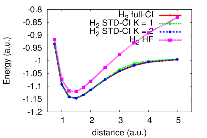
Figure 1: Potential curve of H₂ molecules for full-CI (solid line), STD-CI with $K=1$ (broken line with cross) and $K=2$ (broken line with asterisk), and HF (dotted line).

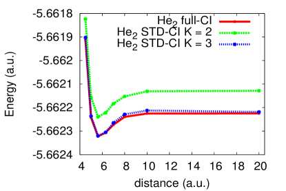
Figure 2: Potential curve of He₂ molecules for full-CI (solid line) and STD-CI with $K=2$ (broken line with cross) and $K=3$ (broken line with asterisk).

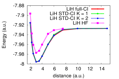
Figure 3: Potential curve of LiH molecules for full-CI (solid line), STD-CI with $K=1$ (broken line with cross) and $K=2$ (broken line with asterisk), and HF (dotted line).

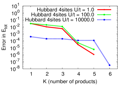
Figure 4: Error in E_tot for the four-site Hubbard model for various parameters $U/t=1$ (solid line), $U/t=100$ (dotted line with cross), and $U/t=10000$ (dotted line with asterisk).

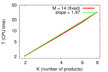
Figure 5: Total CPU time ($T$) versus $K$. The solid line indicates result after measurement for one iteration step and broke line indicates that after fitting to $T=aK^{b}$. $b$ is obtained as 1.97.

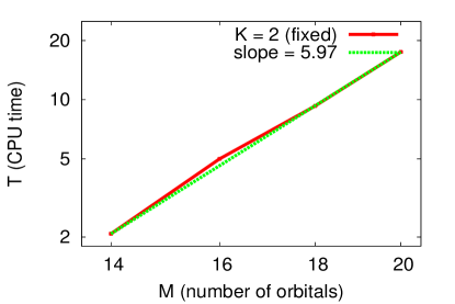
Figure 6: Total CPU time ($T$) versus $M$. The solid line indicates result after measurement for one iteration step and the broken line indicates that after fitting to $T=aM^{b}$. $b$ is 5.97 after the fitting.

We formulated a practical scheme to perform the full-CI level calculation using the STD method. In the STD-CI method, we expand the CI coefficients as the product of a symmetric tensor and the permutation tensor, and we further expand the symmetric tensor into Kronecker product states composed of vectors of dimension $M$. By varying the vectors and the unitary transformation matrix $U_{ij}$, the total energy is minimized using the second-order density matrix technique. The STD-CI method, which involves taking the length of the series $K$ as the only input parameter, allows us to perform a full-CI level calculation rigorously using $KM+M\left(M+1\right)/2$ variational parameters and $\sim K^{2}M^{6}$ operations. By applying the scheme to the potential curve of small diatomic molecules such as H₂, He₂, and LiH, and the four-site Hubbard model for various parameters, we found that a very small $K$ value is required to reproduce the full-CI results within milli-Hartree accuracy. If $K$ increases moderately with $N$, $M$, or the degree of correlation, the scheme will greatly extend the applicability of the full-CI level calculation. We believe that application of the scheme to a crystalline solid and the use of the scheme as a building block of the fragment molecular orbital (FMO) scheme can be of high significanceFMO .

Acknowledgement

The authors thank Prof. Y. Mochizuki (Rikkyo Univ.) and M. Nakata (RIKEN) for their valuable discussions.

References

- (1) I. Shavitt, Mol. Phys., 94, 3 (1998).
- (2) J. Cízek, J. Chem. Phys., 45, 4256 (1966); Adv. Chem. Phys., 14, 35 (1969).
- (3) J. Cízek and J. Paldus, Int. J. Quantum Chem., 5, 359 (1971).
- (4) M. Nakata, H. Nakatsuji et al., J. Chem. Phys. 116, 5432 (2002).
- (5) S. R. White, Phys. Rev. Lett. 69, 2863 (1992).
- (6) S. Rommer and S. Ostlund, Phys. Rev. B 55, p.2164 (1997).
- (7) S. Daul and I. Ciofini et al., I. J. Q. Chem. 79, 331(2000).
- (8) S. Sharma and G. K-L. Chan, J. Chem. Phys. 136, 124121 (2012).
- (9) K. H. Marti, B. Bauer, M. Reiher, M. Troyer, and F. Verstraete, New J. Phys., 12 103008 (2010).
- (10) K. H. Marti and M. Reiher, Phys. Chem. Chem. Phys., 13, 6750 (2011).
- (11) F. Hitchcock, J. Math. Phys. 6, 164 (1927); ibid 7, 9 (1927).
- (12) L. R. Tucker, Psychometrika 31, 279 (1966).
- (13) J. D. Carroll and J. J. Chang, Psychometrika, 35 283 (1970).
- (14) R. A. Harshman, UCLA Working Papers in Phonetics, 16, 1 (1970).
- (15) F. Bell, D. S. Lambrechta and M. Head-Gordon, Mol. Phys. 108, 2759 (2010).
- (16) U. Benedikt, A. A. Auer, M. Espig, and W. Hackbusch, J. Chem. Phys. 2134, 054118 (2011).
- (17) D.C. Kay, “tensor Calculus. Schaum’s Outlines”, McGraw Hill (USA) (1988),
- (18) F. Viète, Opera mathematica, edited by F. van Schooten p. 162 (1579). Reprinted Leiden, Netherlands (1646).
- (19) M. Hasse, J. Appl. Math. Mech., 40, 523 (1960).
- (20) N. E. Brener and J. L. Fry, Phys. Rev. B17, 506 (1978).
- (21) J. L. Fry, N. E. Brener, and R. K. Bruyere, Phys. Rev. B16, 5225 (1977).
- (22) T. van Mourik, A. K. Wilson and T. H. Dunning JR, Mol. Phys., 96, 529 (1999).
- (23) U. Kleinekathofer, K. T. Tang et al., Chem. Phys. Lett., 249, 257(1996).
- (24) K. Kitaura, E. Ikeo, T. Asada, T. Nakano and M. Uebayasi, Chem. Phys. Lett., 313, 701 (1999).