Aligned Spins: Orbital Elements, Decaying Orbits, and Last Stable Circular Orbit to high post-Newtonian Orders

Abstract

In this article the quasi-Keplerian parameterisation for the case that spins and orbital angular momentum in a compact binary system are aligned or anti-aligned with the orbital angular momentum vector is extended to 3PN point-mass, next-to-next-to-leading order spin-orbit, next-to-next-to-leading order spin(1)-spin(2), and next-to-leading order spin-squared dynamics in the conservative regime. In a further step, we use the expressions for the radiative multipole moments with spin to leading order linear and quadratic in both spins to compute radiation losses of the orbital binding energy and angular momentum. Orbital averaged expressions for the decay of energy and eccentricity are provided. An expression for the last stable circular orbit is given in terms of the angular velocity type variable $x$.

1 Introduction

Recent progresses in the post-Newtonian treatment of compact binary systems with spinning components call for an extension of the known parametric solutions to the binary dynamics to include latest spin interaction terms as well as radiative dynamics. As computer resources are recently unable to generate thousands of orbits, which are interesting to ELISA (which may be, optimistically, able in a few decades to see gravitational waves of orbital periods of a few hours), it is desirable to have accurate and efficient gravitational wave templates for an analysis of the detector data. In a prequel paper [1] reasons can be found why to regard compact binary systems with aligned spins with regard to their implications to gravitational wave data analysis. This article will aim to incorporate higher-order terms to the in the orbital and spin dynamics to the quasi-Keplerian parameterisation for compact binaries with aligned spins. These may become interesting when the binaries come to the final stage of their life before merger.

Let us state why we concentrate on the case of “up-up”, “down-down” or any mixed alignments of the spins ${\mathbf{S}}_{1}$ and ${\mathbf{S}}_{2}$ with respect to the orbital angular momentum ${\mathbf{L}}$. In case that the spins are not aligned, we have to deal with spin precession equations, whose analytic solutions are not known in general. A special treatment of, for example, canonical transformations with the help of Lie series is required to shift oscillatory parts of the precession equations of motion to a sufficiently high order in (a special choice of) the perturbation smallness parameter. That would exceed the aim of this article and will be treated in a forthcoming publication.

We confirm our goal to deal with aligned spins by stating that those sources are the “loudest” sources of gravitational waves in the sense of Ref. [2] and are of the high physical importance, because a number of effects as already listed in Ref. [1] arrange it so that the final configuration of the spins is that of alignment. At last, aligned spins are, despite the complicated expressions, still treatable with the help of the quasi-Keplerian parameterisation in an analytical manner.

The present publication will provide analytical expressions for the elements of the quasi-Keplerian parameterisation (QKP) to all the conservative orders we listed in the abstract, and it will also provide first time derivatives of selected orbital elements due to gravitational wave emission incorporating leading-order spin-orbit, spin(1)-spin(2) and spin-squared dynamics.

Let us give a reason why we included S²-effects, although they may be negligible for neutron stars having spin parameters $a\lesssim 0.1$. In contrast, the spin parameters of black holes are allowed to be in the region $a\lesssim 1$, and the spin of non-compact objects – like the sun – are even larger, say $a\sim 4$ and do affect the binary motion. As we regard rotational deformation, we have to include those kinds of effects. Furthermore, although these interactions are weak compared to point-particle contributions, they are even stronger than spin(1)-spin(2) interactions and will lead to modifications in the long-term evolution of gravitational-wave signals.

The mathematical context of the orbital elements describing the motion in the orbital plane will be given in Eqs. (19) – (22). For better readability of the article, we list the most important terms in a small table below.

Quantity	Description	Defined in	Result
$c^{-1}$	Power counting for post-Newtonian orders, mostly set to 1
$n$PN	$n^{\rm th}$ post-Newtonian order, ${\cal O}({c}^{-2n})$
$\delta_{\rm{S}}$	Spin power counting, mostly set to 1
$\chi_{a}$	Projection of object $a$’s spin onto ${\mathbf{e}}_{z}$: $\chi_{a}:=({\mathbf{S}}_{a}\cdot{\mathbf{e}}_{z})$
$\eta$	Symmetric mass ratio: $\eta:=m_{1}m_{2}/(m_{1}+m_{2})^{2}$
$x$	Quantity related to orbital angular velocity
$|E|$	Absolute value of binding energy
$L$	Angular momentum of orbit, $L:=|{\mathbf{L}}|$
${\cal M}$	Mean anomaly	Eq. (19)
${\cal N}$	Mean motion or radial angular velocity, respectively	Eq. (20)	Eq. (28)
${\cal E}$	Eccentric anomaly	Eq. (20)
$v$	True anomaly	Eq. (22)
$\phi$	Elapsed phase as function of ${\cal E}$	Eq. (21)
${\mathbf{S}}_{a}$	Spin vector of object $a$
$S_{a(i)(j)}$	Spin tensor of object $a$ , $S_{a(i)(j)}=\frac{1}{2}\epsilon_{ijk}S^{k}_{a}$ (harmonic and canonical)	Eq. (38)
$C_{Qa}$	Quadrupole constant of object $a$
${\cal I}_{i_{N}}$	Mass-type multipole moments	Eqs. (41)-(45)
${\cal J}_{i_{N}}$	Current-type multipole moments	Eqs. (46)-(49)
$a_{r}$	Semimajor axis	Eq. (19)	Eq. (24)
$e_{r}$	Radial eccentricity	Eq. (19)	Eq. (LABEL:Eq::erSq)
$e_{t}$	Time eccentricity	Eq. (20)	Eq. (25)
$P=:\frac{2\pi}{{\cal N}}$	Radial period	Eq. (19)	Eq. (28)
$\Phi$	Total Phase elapsed between 2 successive periastron passages	Eq. (21)	Eq. (33)
$e_{\phi}$	Phase eccentricity	Eq. (22)	Eq. (LABEL:Eq::ephiSq)
$\langle\frac{\rmd|E|}{\rmd t}\rangle$	Orbital-averaged decay of energy	Eq. (58)	Eq. (64)
$\langle\frac{\rmd e_{r}}{\rmd t}\rangle$	Orbital-averaged decay of eccentricity	Eq. (58)	Eq. (65)

Table 1: List of used quantities in this article: definitions and where to find results.

The other orbital elements of the Kepler equation (20), namely $F_{v},F_{2v},F_{3v}$, and $F_{v-u}$ can be found in Eqs. (29), (30), (31), and (32), while the further elements of the orbital phase, (21), $G_{2v}$, $G_{3v}$, $G_{4v}$, and $G_{5v}$ can be found in Eqs. (34), (35), (36), and (37) in order of appearance.

Let us, for convenience, state some milestones in the recent literature. For literature on point-mass Hamiltonians through 3PN and leading-order spin-squared and spin-orbit Hamiltonians, we refer the reader to the introduction of our previous paper [1] and start from there. Note that there were two recent publications concerning the 4PN conservative point-mass dynamics (see [3] for the 4PN Lagrangean and [4] for the Hamiltonian in the center-of-mass frame, both as preliminary results up to order $G^{2}$).

The next-to-leading order (NLO) spin-orbit (SO) contributions have been derived in [5] and later in [6]. Next-to-next-to-leading order (NNLO) spin-orbit and spin(1)-spin(2) (S(1)S(2)) Hamiltonians are recently derived in [7, 8] and the corresponding Lagrangian potential via the effective field theory formalism in [9] and will also be used in our calculation. The leading-order S(1)S(2) Hamiltonians are available in [10] and extended to NLO in [11]. Spin-squared dynamics (S(1)², S(2)²) depend on the model – or more precisely on the equation of state – of the matter of the constituents of the binary. Depending on its rotational velocity and its stiffness, the included body will deform and self-induce a spin quadrupole moment that will start interacting with the binary orbit and re-couple to the gravitational field. The proportionality factor $C_{{\rm Q}a}$ will represent this issue. It varies from one of black holes to four for neutron stars (such that it is related to the constant $\lambda_{a}$ of object $a$ in Ref. [1] via $C_{{\rm Q}a}=-2\lambda_{a}$) and thus characterises how a body resists rotational deformation. References [12, 13] provide the NLO interactions of this type.

Anyway, as the spins do not precess, the quasi-Keplerian parameterisation [14, 15] can be employed to obtain a parametric solution to the dynamics. When the spins are not aligned, their orientation is not constant. There exist several publications about precessing spins, see e.g. [16] for the case of “simple precession” (which means circular orbits together with the fact that the angle between the total angular momentum ${\mathbf{J}}={\mathbf{L}}+{\mathbf{S}}_{1}+{\mathbf{S}}_{2}$ and ${\mathbf{L}}$ is conserved), [17, 18, 19] for the case that only one body is spinning or the masses are equal, and [20] for circular binaries with unequal masses.

As gravitational waves carry away energy and angular momentum, the semimajor axis and the orbital eccentricity will suffer a slow decay in the validity regime of the post-Newtonian approximation. The radiative losses of compact binaries have been extensively discussed in the literature. Reference [21] gives a general expression for the losses due to gravitational waves in terms of the mass and current-type multipole moments of the binary. This has been elaborated in general in [22] and applied to non-spinning compact binaries in [23] through 2PN point particle dynamics, and, recently, in [24] to 3PN point particle dynamics. In Section 5 we give expressions for the decay of the orbital energy and the radial eccentricity, deduced from the spin dependent multipole moments given in [21] and [25].

Since we used different approximation levels for the last stable circular orbit calculations, the quasi-Keplerian parameterisation, and the radiative dynamics they will be applied exclusively in the corresponding sections. This is due to the fact that the conservative and dissipative effects are known for the spin up to different approximation levels. The NNLO spin-orbit Hamiltonian completes the knowledge of the dynamics of binary black holes up to and including 3.5PN for maximally rotating objects. For general compact objects like neutron stars the leading order spin(1)³ Hamiltonians are still missing. Since the NNLO S(1)S(2) Hamiltonian is at 4PN if both objects are rapidly rotating, the full post-Newtonian approximate dynamics up to and including 4PN requires further efforts.

The structure of the paper is as follows. First of all the determination of the last stable circular orbit and a resummed binding energy will be discussed in Section 2. Afterwards in Section 3 a quick summary of the quasi-Keplerian parameterisation for eccentric orbits and the appropriate orbital elements will be given. In Section 5 the dissipative dynamics and energy and angular momentum loss will be discussed. Finally, in Section 6 the conclusions and future applications will be provided. The reader will find short subsection of the rescaling of several quantities to simplify equations and discussions in the appendix. As well, we provided a general discussion about the stability of the chosen configuration.

2 Last Stable Circular Orbit

To determine the last stable circular orbit our starting point is the binding energy for circular orbits. Either one can extract it from a Lagrangian potential constructed from a given metric or one can get the binding energy from a Hamiltonian in the center-of-mass frame for circular motion. This means in the center-of-mass frame Hamiltonian the $p_{r}=({{{\mathbf{n}}}_{12}}\cdot{\hat{{\mathbf{p}}}})$ component of the linear momentum must be set to zero and ${\hat{{\mathbf{p}}}}^{2}=L^{2}/r^{2}$ holds. For a system with spins we further set the spins to a configuration in which they are aligned with the orbital angular momentum. For an energy $E(r,L)$ the circular orbit is given by the perturbative solution of

$$\frac{\partial E}{\partial r}(r,L) = 0\,,$$ (1)

for $L$. Then $E(r,L(r))$ is the binding energy at the circular orbit $r$. Since the radial coordinate depends on a certain gauge we have to transform it into a gauge invariant quantity (invariant under a large class of gauge transformations, see [26, 27, 28]) given by

$$x = \left(\frac{\partial E}{\partial L}(r,L(r))\right)^{2/3}\,,$$ (2)

which is related to the orbital angular velocity, see Table 1 in the introduction and A. For the Schwarzschild spacetime the binding energy for a circular orbit is given by

$$E_{{\rm Schw}}(x) = \frac{1-2x}{\sqrt{1-3x}}-1\,.$$ (3)

For a test-spin in a stationary Kerr spacetime we can also write down this expression for orbital momentum aligned Kerr spin and test-spin to linear order in test-spin (see [29, 30, 31] for the appropriate potentials), namely

$$E_{{\rm Kerr,TS}}(x) = -1-\frac{2}{\sqrt[6]{-a+x^{-3/2}}\sqrt{a+x^{-3/2}-3\sqrt[3]{-a+x^{-3/2}}}}$$ (4)

$$+\frac{x^{-3/2}}{\sqrt{-a+x^{-3/2}}\sqrt{a+x^{-3/2}-3\sqrt[3]{-a+x^{-3/2}}}}$$

$$+S\frac{\left(-a+\sqrt[3]{-a+x^{-3/2}}\right)x^{3/2}}{\sqrt{-a+x^{-3/2}}\sqrt{a+x^{-3/2}-3\sqrt[3]{-a+x^{-3/2}}}\left(ax^{3/2}-1\right)}\,.$$

In the post-Newtonian case one can also write down this binding energy, but we will not provide it here since the expression is very lengthy and gives no further deep insights into the calculation (see e.g. [32] for very recent results). We briefly note that it is a polynomial in $\sqrt{x}$ which corresponds to a post-Newtonian expansion. From the binding energy for circular orbits $E(x)$ we constructed a quantity $e(x)$ via

$$e(x) = \left[\frac{(\eta E(x)+1)^{2}-1}{2\eta}+1\right]^{2}-1\,,$$ (5)

(see e.g. [33]). We refer to $e(x)$ as “modified binding energy” in contrast to “binding energy” in case of $E(x)$. The modified binding energy $e(x)$ has for a test-mass ($\eta=0$) moving in a Schwarzschild spacetime a polynomial structure in $x$ in the numerator and denominator. In contrast, this is not true for the binding energy $E(x)$, see Eq. (3). For the modified binding energy of a test-spin moving in the equatorial plane of a stationary Kerr black hole this is not true either, see below in Eq. (7). The relation between the $\chi_{1}$, $\chi_{2}$ spin magnitudes and $a$, $S$ is given by $\chi_{1}=a$ and $\chi_{2}=S/\eta$. Notice that the $1/\eta$ terms are not singular, because $1-\sqrt{1-4\eta}=4\eta/(1+\sqrt{1-4\eta})$, which renders these terms well-defined at $\eta=0$. This issue appears due to the fact that $S$ is a test-spin and so may not vanish in the limit $\eta\to 0$. Here one has to approximate in Kerr spin and test-spin to get a rational structure. The mentioned modified binding energies are given by

$$e_{{\rm Schw}}(x) = -x\frac{1-4x}{1-3x}\,,$$ (6)

$$e_{{\rm Kerr,TS}}(x) = \frac{-\sqrt[3]{-a+x^{-{3}/{2}}}x^{{3}/{2}}+x^{3}\bigl{(}a^{2}-3a\sqrt[3]{-a+x^{-{3}/{2}}}+4\sqrt[3]{-a+x^{-{3}/{2}}}^{2}\bigr{)}}{\left(-1+ax^{{3}/{2}}\right)\biggl{(}-1+x^{{3}/{2}}\Bigl{(}-a+3\sqrt[3]{-a+x^{-{3}/{2}}}\Bigr{)}\biggl{)}}$$ (7)

$$-2S\frac{x^{3}\left(-a+\sqrt[3]{-a+x^{-3/2}}\right)\left(-1+2\sqrt[3]{-a+x^{-3/2}}x^{3/2}\right)}{\left(-1+ax^{3/2}\right)^{2}\left(-1+\left[-a+3\sqrt[3]{-a+x^{-3/2}}\right]x^{3/2}\right)}\,.$$

In the approximation in Kerr spin and test-spin the modified binding energy reads

$$e_{{\rm approx.Kerr,TS}}(x) = -x\frac{{1-4x}+\frac{8}{3}ax^{3/2}-a^{2}x^{2}+\frac{8}{3}ax^{5/2}-\frac{10}{9}a^{2}x^{3}+\frac{4}{9}a^{2}x^{4}}{{1-3x}+4ax^{5/2}-a^{2}x^{3}-\frac{2}{3}a^{2}x^{4}{+2Sx^{5/2}-2aSx^{3}+2Sx^{7/2}-\frac{2}{3}aSx^{4}}}\,,$$ (8)

where one can still identify the terms coming from the test-mass motion in a Schwarzschild spacetime. (Notice that the test-spin parts in the denominator were implemented by using the geometric series at first order, i.e. $1/(1-x)\approx 1+x$, to implement the correct pole structure coming from the test-spin.) In summary, by using an approximation in Kerr spin and test-spin, we were able to construct a rational function of $\sqrt{x}$ appearing in Eq. (8) similar to the Schwarzschild case Eq. (6). This rational function in $\sqrt{x}$ can be taken as a starting point to interpolate between modified binding energy for a test-spin in Kerr spacetime and post-Newtonian approximate expression for a gravitating mass orbiting another gravitating mass.

2.1 Construction of Binding Energy

After having an initial guess for the rational modified binding energy we tuned all parts of the numerator by $\eta$-dependent coefficients and matched the Taylor expansion in $\sqrt{x}$ with the post-Newtonian approximated $e(x)$ obtained from the ADM-Hamiltonians (3PN point-mass, NNLO spin-orbit, NNLO S(1)S(2), NLO spin-squared). These considerations lead to the expression

$$e_{{\rm tunedKerr,TS}}(x) =-x\biggl{[}1-\left(4+\frac{\eta}{3}\right)x+a\left(-\frac{2\eta}{3}+\frac{4}{3}+\frac{4}{3}\sqrt{1-4\eta}\right)x^{3/2}+S\left(-\frac{2}{3}+\frac{4}{3\eta}(1-\sqrt{1-4\eta})\right)x^{3/2}$$ (9)

$$\quad+\left(\frac{47\eta}{12}-2aS+a^{2}C_{Q1}\left(\eta-\frac{1}{2}-\frac{1}{2}\sqrt{1-4\eta}\right)\right)x^{2}$$

$$\quad+a\left(\frac{4\eta^{2}}{9}-\frac{91\eta}{18}+\frac{10}{3}-\sqrt{1-4\eta}\left(\frac{43\eta}{18}+\frac{2}{3}\right)\right)x^{5/2}$$

$$\quad+S\left(\frac{4\eta}{9}-\frac{55}{18}+\frac{43}{18}\sqrt{1-4\eta}+\frac{2}{3\eta}(\sqrt{1-4\eta}-1)\right)x^{5/2}$$

$$\quad+\left(\frac{\eta^{3}}{81}-\frac{103\eta^{2}}{36}-\frac{205\pi^{2}\eta}{96}+\frac{3679\eta}{72}\right)x^{3}+aS\left(\frac{4\eta}{9}+\frac{10}{3}\right)x^{3}$$

$$\quad+a^{2}\left(C_{Q1}\left(-\frac{4\eta^{2}}{3}+\frac{14\eta}{3}-\frac{7}{6}\right)-\frac{10\eta^{2}}{9}-\frac{5\eta}{18}+\frac{1}{9}+\sqrt{1-4\eta}\left(C_{Q1}\left(\frac{7\eta}{3}-\frac{7}{6}\right)+\frac{35\eta}{18}+\frac{10}{9}\right)\right)x^{3}$$

$$\quad+a\left(\frac{95\eta^{2}}{6}-\frac{197\eta}{8}-2+\sqrt{1-4\eta}\left(\frac{3\eta^{2}}{2}-\frac{463\eta}{24}+2\right)\right)x^{7/2}$$

$$\quad+S\left(\frac{91\eta}{6}-\frac{559}{24}+\sqrt{1-4\eta}\left(-\frac{3\eta}{2}+\frac{463}{24}\right)+\frac{2}{\eta}(1-\sqrt{1-4\eta})\right)x^{7/2}$$

$$\quad+\biggl{(}F(\eta)+aS\left(\frac{92\eta^{2}}{27}+\frac{202\eta}{9}-8+\frac{8}{3}\sqrt{1-4\eta}+\frac{16}{3\eta}(1-\sqrt{1-4\eta})\right)$$

$$\quad\quad+\frac{4}{9}a^{2}f_{7}(\eta)\biggr{)}x^{4}\left.\biggr{]}\right/\biggl{[}1-3x+(4a+2S)x^{5/2}-(a^{2}+2aS)x^{3}+2Sx^{7/2}-\frac{2}{3}(a^{2}+aS)x^{4}\biggr{]}\,.$$

There are no quadratic terms in the test-spin, so there will be no $C_{Q2}$ in the expression. However, $S$ is a test-spin and the denominator of $e(x)$ is only valid in the test-spin limit, hence the results given here are only valid around $\eta\approx 0$. The unknown function $F(\eta)$ has to be fixed by the 4PN point-mass Hamiltonian later (see [3] and [4]) and the unknown function $f_{7}(\eta)$ by the NNLO S(1)² Hamiltonian ( $f_{7}(\eta)\stackrel{{\scriptstyle\eta\to 0}}{{\longrightarrow}}1$ is required to be consistent with the Kerr-limit).

We wish to mention Ref. [34] where self-force corrections to the binding energy for circular orbits have been computed and also Ref. [35] where the resulting energy has been compared to post-Newtonian theory and numerical relativity.

The equation ${\rm d}e_{{\rm tunedKerr,TS}}(x)/{\rm d}x=0$ is numerically solved and one can obtain the solution $x_{{\rm LSO}}$ for certain mass ratios $\eta$, spins and quadrupole constants, see Figure 1.

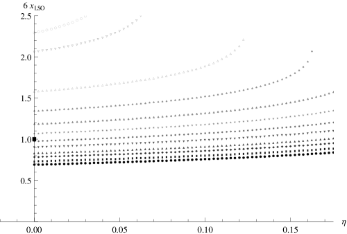
Figure 1: Last stable circular orbit for $S=0.1$ plotted for different symmetric mass ratios $\eta$ and Kerr spins $a$. (From black to light grey $a=-1.0$ to $a=0.84$. The two uppermost plots contain the cases $a=0.8$ and $a=0.84$ respectively. The difference in Kerr spin between all other plots is $\Delta a=0.2$.) The black square ($\blacksquare$) denotes the last stable circular orbit of a testmass orbiting a Schwarzschild black hole. Also notice that continuation to large Kerr spins $a$ is invalid because the last stable circular orbit will be of the order of magnitude of the Schwarzschild radius which violates the post-Newtonian approximation (wide separation). The reader should be reminded that the frequency-type quantity $x$ increases as the radius of a circular orbit decreases.

To link to recent literature, we wish to mention reference [33] where the last stable circular orbit through third post-Newtonian order for point masses has been computed. To generalise to certain configurations including spin, the binding energy of “last stable spherical orbits” has been derived, for example, in [36] in the effective one-body approach for non-aligned spins. Compact binaries with spin under NLO spin-orbit coupling evolving in circular orbits were studied in [37]. We also wish to reference [38] where corrections to the last stable circular orbit of a Schwarzschild black hole due to the gravitational self-force have been derived, and also [39] where the authors calculated gravitational self-force corrections to strongly bound eccentric orbits in a Schwarzschild spacetime.

3 Eccentric Orbits: Calculation Of The Quasi-Keplerian Parameterisation

3.1 Included Hamiltonians

The NNLO spin-orbit [7], the NLO S(1)S(2) [40] and NNLO S(1)S(2) [8], and finally the NLO S(1)² Hamiltonian [13] in reduced form (in the center of mass) are listed below. The point-mass and LO spin-orbit, S(1)S(2), and spin-squared Hamiltonians can be found in [1]. We define the sums and differences of the two canonical spin tensors as

$$\hat{\Sigma}_{ij} := \hat{S}_{1\,(i)(j)}+\hat{S}_{2\,(i)(j)}\,,$$ (10)

$$\hat{\Delta}_{ij} := \hat{S}_{1\,(i)(j)}-\hat{S}_{2\,(i)(j)}\,,$$ (11)

labeled with a “hat”. Those satisfying the covariant spin supplementary condition will be labeled with a “tilde”, namely

$$\tilde{\Sigma}_{ij} := \tilde{S}_{1\,(i)(j)}+\tilde{S}_{2\,(i)(j)}\,,$$ (12)

$$\tilde{\Delta}_{ij} := \tilde{S}_{1\,(i)(j)}-\tilde{S}_{2\,(i)(j)}\,,$$ (13)

and the latter will become important for the multipole moment expressions taken from the literature. The reduced Hamiltonians read

$${\rm H}_{\rm{SO}}^{\rm{NNLO}} = \frac{\delta_{S}}{c^{6}}\Biggl{\{}\frac{1}{r^{3}}\Biggl{[}\left(\frac{275\eta^{2}}{32}-8\eta\right)({\mathbf{p}}\cdot{{{\mathbf{n}}}_{12}})^{2}\left({n}_{12}^{i}p^{j}\hat{\Sigma}_{ij}\right)+\sqrt{1-4\eta}\left({n}_{12}^{i}p^{j}\hat{\Delta}_{ij}\right)\biggl{(}\frac{-\eta}{32}(45\eta+256)({\mathbf{p}}\cdot{{{\mathbf{n}}}_{12}})^{2}$$ (14)

$$-\frac{\eta}{32}(39\eta+314){({\mathbf{p}}^{2})}\biggr{)}+\frac{\eta}{32}(73\eta-206)\left({n}_{12}^{i}p^{j}\hat{\Sigma}_{ij}\right){({\mathbf{p}}^{2})}\Biggr{]}+\frac{1}{r^{2}}\Biggl{[}\frac{-15}{32}\eta^{2}(2\eta-1)({\mathbf{p}}\cdot{{{\mathbf{n}}}_{12}})^{4}\left({n}_{12}^{i}p^{j}\hat{\Sigma}_{ij}\right)$$

$$-\frac{3}{32}\eta\left(6\eta^{2}-11\eta+4\right)({\mathbf{p}}\cdot{{{\mathbf{n}}}_{12}})^{2}\left({n}_{12}^{i}p^{j}\hat{\Sigma}_{ij}\right){({\mathbf{p}}^{2})}+\sqrt{1-4\eta}\left({n}_{12}^{i}p^{j}\hat{\Delta}_{ij}\right)\biggl{(}\frac{15\eta^{2}({\mathbf{p}}\cdot{{{\mathbf{n}}}_{12}})^{4}}{32}$$

$$+\frac{3}{32}\eta(9\eta-4)({\mathbf{p}}\cdot{{{\mathbf{n}}}_{12}})^{2}{({\mathbf{p}}^{2})}+\frac{1}{16}\eta(22\eta-9){({\mathbf{p}}^{2})}^{2}\biggr{)}-\frac{1}{16}\eta\left(5\eta^{2}-3\eta+2\right)\left({n}_{12}^{i}p^{j}\hat{\Sigma}_{ij}\right){({\mathbf{p}}^{2})}^{2}\Biggr{]}$$

$$+\frac{1}{r^{4}}\biggl{[}\frac{1}{8}\left(-2\eta^{2}+33\eta+42\right)\left({n}_{12}^{i}p^{j}\hat{\Sigma}_{ij}\right)+\frac{21}{4}\sqrt{1-4\eta}(\eta+1)\left({n}_{12}^{i}p^{j}\hat{\Delta}_{ij}\right)\Biggr{]}\Biggr{\}}\,,$$

$${\rm H}_{\rm{S(1)S(2)}}^{\rm{NLO}} = \frac{\delta_{S}^{2}}{c^{4}}\Biggl{\{}\frac{1}{{r}^{3}}\Biggl{[}_{3}-\frac{15}{2}\eta^{2}{({\mathbf{p}}\cdot{{{\mathbf{n}}}_{12}})}^{2}{\left({n}_{12}^{j}{n}_{12}^{k}\hat{S}_{1\,(j)(q)}\hat{S}_{2\,(k)(q)}\right)}+{\left(\hat{S}_{1\,(j)(k)}\hat{S}_{2\,(j)(k)}\right)}\frac{\eta^{2}}{2}\left(3{({\mathbf{p}}\cdot{{{\mathbf{n}}}_{12}})}^{2}+{{({\mathbf{p}}^{2})}}\right)$$ (15)

$$-\frac{3}{2}\eta^{2}{\left({n}_{12}^{j}{n}_{12}^{k}\hat{S}_{1\,(j)(q)}\hat{S}_{2\,(k)(q)}\right)}{{({\mathbf{p}}^{2})}}+\frac{\eta^{2}}{4}{\left(p^{j}p^{k}\hat{S}_{1\,(j)(q)}\hat{S}_{2\,(k)(q)}\right)}$$

$$+{({\mathbf{p}}\cdot{{{\mathbf{n}}}_{12}})}\frac{3}{4}\Biggl{(}_{1}\left((2\eta+1)\eta+\sqrt{1-4\eta}\eta\right){\left({n}_{12}^{i}\hat{S}_{1\,(i)(q)}p^{j}\hat{S}_{2\,(j)(q)}\right)}$$

$$+\left(\eta(2\eta+1)-\sqrt{1-4\eta}\eta\right){\left({n}_{12}^{i}\hat{S}_{2\,(i)(k)}p^{j}\hat{S}_{2\,(j)(k)}\right)}\Biggr{)}_{1}$$

$$-\frac{3}{4}(\eta+2)\eta{\left({n}_{12}^{i}p^{j}\hat{S}_{1\,(i)(j)}\right)}{\left({n}_{12}^{i}p^{j}\hat{S}_{2\,(i)(j)}\right)}\Biggr{]}_{3}$$

$$+\frac{12\eta}{{r}^{4}}{\left({n}_{12}^{j}{n}_{12}^{k}\hat{S}_{1\,(j)(q)}\hat{S}_{2\,(k)(q)}\right)}-3\eta{\left(\hat{S}_{1\,(j)(k)}\hat{S}_{2\,(j)(k)}\right)}\Biggr{\}}\,,$$

$${\rm H}_{\rm{S(1)S(2)}}^{\rm{NNLO}} = \frac{\delta_{S}^{2}}{c^{6}}\Biggl{\{}\frac{1}{{r}^{4}}\Biggl{[}_{4}\frac{1}{4}\eta^{2}{\left({n}_{12}^{j}{n}_{12}^{k}\hat{S}_{1\,(j)(q)}\hat{S}_{2\,(k)(q)}\right)}\left(303{({\mathbf{p}}\cdot{{{\mathbf{n}}}_{12}})}^{2}+77{{({\mathbf{p}}^{2})}}\right)+\frac{15}{4}\eta^{2}{\left(p^{j}p^{k}\hat{S}_{1\,(j)(q)}\hat{S}_{2\,(k)(q)}\right)}$$ (16)

$$+\frac{1}{4}\eta\left(12(4\eta+3){\left({n}_{12}^{i}p^{j}\hat{S}_{1\,(i)(j)}\right)}{\left({n}_{12}^{i}p^{j}\hat{S}_{2\,(i)(j)}\right)}-\eta{\left(\hat{S}_{1\,(j)(k)}\hat{S}_{2\,(j)(k)}\right)}\left(52{({\mathbf{p}}\cdot{{{\mathbf{n}}}_{12}})}^{2}+23{{({\mathbf{p}}^{2})}}\right)\right)$$

$$+{\left({n}_{12}^{i}\hat{S}_{1\,(i)(q)}p^{j}\hat{S}_{2\,(j)(q)}\right)}\left(-\frac{3}{2}\sqrt{1-4\eta}\eta(\eta+3){({\mathbf{p}}\cdot{{{\mathbf{n}}}_{12}})}-\frac{1}{2}\eta(44\eta+9){({\mathbf{p}}\cdot{{{\mathbf{n}}}_{12}})}\right)$$

$$+{\left({n}_{12}^{i}\hat{S}_{2\,(i)(k)}p^{j}\hat{S}_{2\,(j)(k)}\right)}\left(\frac{3}{2}\sqrt{1-4\eta}\eta(\eta+3){({\mathbf{p}}\cdot{{{\mathbf{n}}}_{12}})}-\frac{1}{2}\eta(44\eta+9){({\mathbf{p}}\cdot{{{\mathbf{n}}}_{12}})}\right)\Biggr{]}_{4}$$

$$+\frac{1}{{r}^{3}}\Biggl{[}_{3}{\left({n}_{12}^{i}\hat{S}_{1\,(i)(q)}p^{j}\hat{S}_{2\,(j)(q)}\right)}\biggl{(}\frac{3}{16}\eta{({\mathbf{p}}\cdot{{{\mathbf{n}}}_{12}})}\left(20\eta^{2}{({\mathbf{p}}\cdot{{{\mathbf{n}}}_{12}})}^{2}+\left(6\eta^{2}+4\eta-3\right){{({\mathbf{p}}^{2})}}\right)$$

$$+\frac{9}{16}\sqrt{1-4\eta}\eta(2\eta-1){({\mathbf{p}}\cdot{{{\mathbf{n}}}_{12}})}{{({\mathbf{p}}^{2})}}\biggr{)}+{\left({n}_{12}^{i}\hat{S}_{2\,(i)(k)}p^{j}\hat{S}_{2\,(j)(k)}\right)}\biggl{(}\frac{3}{16}\eta{({\mathbf{p}}\cdot{{{\mathbf{n}}}_{12}})}\Bigl{(}20\eta^{2}{({\mathbf{p}}\cdot{{{\mathbf{n}}}_{12}})}^{2}$$

$$+\left(6\eta^{2}+4\eta-3\right){{({\mathbf{p}}^{2})}}\Bigr{)}+\frac{9}{16}\sqrt{1-4\eta}(1-2\eta)\eta{({\mathbf{p}}\cdot{{{\mathbf{n}}}_{12}})}{{({\mathbf{p}}^{2})}}\biggr{)}$$

$$+\frac{1}{16}\eta^{2}{\left(p^{j}p^{k}\hat{S}_{1\,(j)(q)}\hat{S}_{2\,(k)(q)}\right)}\left((4\eta+1){{({\mathbf{p}}^{2})}}-6\eta{({\mathbf{p}}\cdot{{{\mathbf{n}}}_{12}})}^{2}\right)$$

$$+\frac{1}{16}\eta\biggl{(}_{1}30\eta^{2}{({\mathbf{p}}\cdot{{{\mathbf{n}}}_{12}})}^{4}{\left(\hat{S}_{1\,(j)(k)}\hat{S}_{2\,(j)(k)}\right)}+{{({\mathbf{p}}^{2})}}\biggl{(}2\eta(3\eta-2){{({\mathbf{p}}^{2})}}{\left(\hat{S}_{1\,(j)(k)}\hat{S}_{2\,(j)(k)}\right)}$$

$$-3\left(4\eta^{2}+17\eta-6\right){\left({n}_{12}^{i}p^{j}\hat{S}_{1\,(i)(j)}\right)}{\left({n}_{12}^{i}p^{j}\hat{S}_{2\,(i)(j)}\right)}\biggr{)}$$

$$-6\eta{({\mathbf{p}}\cdot{{{\mathbf{n}}}_{12}})}^{2}(5\eta{\left({n}_{12}^{i}p^{j}\hat{S}_{1\,(i)(j)}\right)}{\left({n}_{12}^{i}p^{j}\hat{S}_{2\,(i)(j)}\right)}-2(\eta-1){{({\mathbf{p}}^{2})}}{\left(\hat{S}_{1\,(j)(k)}\hat{S}_{2\,(j)(k)}\right)})\biggr{)}_{1}$$

$$-\frac{3}{8}\eta^{2}{\left({n}_{12}^{j}{n}_{12}^{k}\hat{S}_{1\,(j)(q)}\hat{S}_{2\,(k)(q)}\right)}\left(35\eta{({\mathbf{p}}\cdot{{{\mathbf{n}}}_{12}})}^{4}+10(\eta-1){({\mathbf{p}}\cdot{{{\mathbf{n}}}_{12}})}^{2}{{({\mathbf{p}}^{2})}}+(3\eta-2){{({\mathbf{p}}^{2})}}^{2}\right)\Biggr{]}_{3}$$

$$+\frac{1}{r^{5}}\biggl{[}_{5}\frac{3}{4}\eta(10\eta+7){\left(\hat{S}_{1\,(j)(k)}\hat{S}_{2\,(j)(k)}\right)}-\frac{1}{4}\eta(79\eta+105){\left({n}_{12}^{j}{n}_{12}^{k}\hat{S}_{1\,(j)(q)}\hat{S}_{2\,(k)(q)}\right)}\biggr{]}_{5}\Biggr{\}}\,,$$

$${\rm H}_{\rm{S(1)^{2}}}^{\rm{NLO}} = \frac{\delta_{S}^{2}}{c^{4}}\Biggl{\{}\frac{1}{r^{3}}\Biggl{[}_{3}{({\mathbf{p}}\cdot{{{\mathbf{n}}}_{12}})}^{2}{\left({n}_{12}^{j}{n}_{12}^{k}\hat{S}_{1\,(j)(q)}\hat{S}_{1\,(k)(q)}\right)}\left(\frac{15}{8}{C}_{\rm Q1}\eta(2\eta-1)-\frac{15}{8}{C}_{\rm Q1}\sqrt{1-4\eta}\eta\right)$$ (17)

$$+{\left(\hat{S}_{1\,(j)(k)}\hat{S}_{1\,(j)(k)}\right)}\biggl{(}_{1}{({\mathbf{p}}\cdot{{{\mathbf{n}}}_{12}})}^{2}\left(-\frac{3}{16}\eta({C}_{\rm Q1}(4\eta+2)+\eta-4)-\frac{3}{8}({C}_{\rm Q1}-2)\sqrt{1-4\eta}\eta\right)$$

$$+{{({\mathbf{p}}^{2})}}\left(\frac{3}{8}\sqrt{1-4\eta}(({C}_{\rm Q1}-2)\eta+{C}_{\rm Q1})+\frac{1}{16}({C}_{\rm Q1}(6-2\eta(2\eta+3))+3(\eta-4)\eta)\right)\biggr{)}_{1}$$

$$+{({\mathbf{p}}\cdot{{{\mathbf{n}}}_{12}})}{\left({n}_{12}^{j}\hat{S}_{1\,(j)(q)}p^{k}\hat{S}_{1\,(k)(q)}\right)}\left(\frac{3}{4}\eta(-2{C}_{\rm Q1}(\eta-2)+\eta-3)+\frac{3}{4}(4{C}_{\rm Q1}-3)\sqrt{1-4\eta}\eta\right)$$

$$+{\left({n}_{12}^{j}{n}_{12}^{k}\hat{S}_{1\,(j)(q)}\hat{S}_{1\,(k)(q)}\right)}{{({\mathbf{p}}^{2})}}\left(\frac{1}{8}(3{C}_{\rm Q1}(\eta+3)(2\eta-1)-3(\eta-4)\eta)-\frac{3}{8}\sqrt{1-4\eta}({C}_{\rm Q1}(\eta+3)-4\eta)\right)$$

$$+{\left(p^{j}p^{k}\hat{S}_{1\,(j)(q)}\hat{S}_{1\,(k)(q)}\right)}\left(-\frac{1}{4}\eta(3{C}_{\rm Q1}+\eta-3)-\frac{3}{4}({C}_{\rm Q1}-1)\sqrt{1-4\eta}\eta\right)\Biggr{]}_{3}$$

$$+\frac{1}{r^{4}}\Biggl{[}_{4}{\left({n}_{12}^{j}{n}_{12}^{k}\hat{S}_{1\,(j)(q)}\hat{S}_{1\,(k)(q)}\right)}\left(\frac{1}{4}(3{C}_{\rm Q1}(\eta+1)-16\eta+6)+\frac{1}{4}\sqrt{1-4\eta}({C}_{\rm Q1}(9\eta+3)-4\eta+6)\right)$$

$$+{\left(\hat{S}_{1\,(j)(k)}\hat{S}_{1\,(j)(k)}\right)}\left(\frac{1}{4}(-{C}_{\rm Q1}(\eta+1)+3\eta-1)+\frac{1}{4}\sqrt{1-4\eta}(-{C}_{\rm Q1}(3\eta+1)+\eta-1)\right)\Biggr{]}_{4}\Biggr{\}}\,,$$

$${\rm H}_{\rm{S(2)^{2}}}^{\rm{NLO}} = {\rm H}_{\rm{S(1)^{2}}}^{\rm{NLO}}\quad(1\leftrightarrow 2)\,,$$ (18)

where Equation (18) follows from the fact that ${{{\mathbf{n}}}_{12}}$ always appears in a quadratic form and the sign has no influence. Note that the NLO S(1)² potentials have also been computed in [41, 42] and the NLO S(1)S(2) potentials in [43, 44] with the help of the effective field theory. We will incorporate these interactions into the quasi-Keplerian parameterisation in the subsequent subsection.

3.2 Geometrical meaning of the elements of the quasi-Keplerian parameterisation

The quasi-Keplerian parameterisation is the basis of the calculation of the radiation losses. Having polar coordinates ($r,\phi$) for the plane of motion characterised by ${\mathbf{L}}$ and the spin as ${\mathbf{S}}_{a}=\chi_{a}{\mathbf{L}}/L$ for the $a$th object at initial instant of time, we list the elements of the parameterisation schematically without stating technical details of the computation. These can be found in, e.g., [14, 15], [1] and references therein. This parameterisation describes the radial distance $r$ and the elapsed orbital phase $\phi$ as a function of the eccentric anomaly ${\cal E}$ and implicitly provides ${\cal E}$ as a function of time via the Kepler equation, see Eq. (20). A pictorial description of this parameterisation can be found in Figure 2 below. Symbolically, the QKP looks as follows:

$$r = a_{r}\left(1-e_{r}\cos{\cal E}\right)\,,$$ (19)

$${\cal N}(t-t_{0}) = {\cal E}-{e_{t}}\sin{\cal E}+F_{v-{\cal E}}(v-{\cal E})+{F_{v}}\sin v+F_{2v}\sin(2v)+F_{3v}\sin(3v)\,,$$ (20)

$$\frac{2\pi}{\Phi}(\phi-\phi_{0}) = v+G_{2v}\sin(2v)+G_{3v}\sin(3v)+G_{4v}\sin(4v)+G_{5v}\sin(5v)\,,$$ (21)

$$v := 2\arctan\left[\sqrt{\frac{1+e_{\phi}}{1-e_{\phi}}}\tan\frac{{\cal E}}{2}\right]\,.$$ (22)

Let us state the importance of these expressions. To express the gravitational waves emitted by the binary as expressions of the elapsed time one also requires to implement the orbital positions and velocities as functions of time, which one might do with the help of th QKP. Further, to get a more or less explicit time dependency of the radiation reaction equations of energy and angular momentum, it is needed to re-express the luminosity and angular momentum loss – which are given in general terms of ${\mathbf{v}}^{2}$, $\dot{r}$, and $r$ – with the help of Equations (19) – (22). Note that the Kepler equation (20) cannot be inverted by $t-t_{0}$ without use of infinite series.

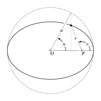
Figure 2: The motion of the reduced mass (black dot) on an ellipse in the Newtonian case. $O$ denotes the origin and $F$ is one focus of the ellipse. Note that $v$ is not identical to the phase $\phi$ in the post-Newtonian case and loses its meaning as the angle between ${{{\mathbf{n}}}_{12}}{}$ and ${\mathbf{e}}_{x}$. The area enclosed by the ellipse, the $x$-axis and the vector ${\mathbf{r}}$ in the first quadrant equals the quantity ${\cal N}(t-t_{0})$. This figure is taken from [15] and modified appropriately.

4 Results for the orbital elements

4.1 Semimajor axis and eccentricities

Let us define $e_{\rm N}$ as the “Newtonian” value of the orbital eccentricity,

$$e_{\rm N}:=\sqrt{1-2|E|L^{2}}\,.$$ (23)

Then, the orbital elements read as follows.

$$a_{r} = \frac{1}{2|E|}+\frac{1}{c^{2}}\Biggl{\{}\frac{\eta-7}{4}\Biggr{\}}+\frac{1}{c^{4}}\Biggl{\{}\frac{11\eta-17}{4L^{2}}+\frac{1}{8}\left(\eta^{2}+10\eta+1\right)|E|\Biggr{\}}$$ (24)

$$+\frac{\delta_{S}}{c^{2}L}\Biggl{\{}\sqrt{1-4\eta}\left(\chi_{1}-\chi_{2}\right)+\left(1-\frac{\eta}{2}\right)\left(\chi_{1}+\chi_{2}\right)\Biggr{\}}$$

$$+\frac{\delta_{S}^{2}}{c^{2}L^{2}}\Biggl{\{}\frac{1}{4}{C}_{\rm Q1}(2\eta-\sqrt{1-4\eta}-1)\chi_{1}^{2}+\frac{1}{4}{C}_{\rm Q2}(2\eta+\sqrt{1-4\eta}-1)\chi_{2}^{2}-\eta\chi_{2}\chi_{1}\Biggr{\}}$$

$$+\frac{\delta_{S}}{c^{4}}\Biggl{\{}\frac{1}{L^{3}}\Biggl{[}_{3}{\left(\chi_{1}-\chi_{2}\right)}\left(8-\frac{9\eta}{4}\right){\sqrt{1-4\eta}}+\left(\eta^{2}-\frac{39\eta}{4}+8\right){\left(\chi_{1}+\chi_{2}\right)}\Biggr{]}_{3}$$

$$+\frac{|E|}{8L}\left[{\left(\chi_{1}-\chi_{2}\right)}(5\eta-8){\sqrt{1-4\eta}}+\left(-6\eta^{2}+19\eta-8\right){\left(\chi_{1}+\chi_{2}\right)}\right]\Biggr{\}}$$

$$+\frac{\delta_{S}^{2}}{c^{4}}\Biggl{\{}\frac{\chi_{1}^{2}}{2}\Biggl{(}\frac{2}{{L}^{4}}\biggl{[}_{4}{{C}_{\rm Q1}}\left(\frac{1}{4}\left(-6\eta^{2}+41\eta-18\right)+\left(\frac{5\eta}{4}-\frac{9}{2}\right){\sqrt{1-4\eta}}\right)-2\left(\eta^{2}-9\eta+3\right)+(6-6\eta){\sqrt{1-4\eta}})\biggr{]}_{4}$$

$$+\frac{2|E|}{{L}^{2}}\left({{C}_{\rm Q1}}\left((\eta-1)^{2}+{\sqrt{1-4\eta}}\right)-\frac{3\eta{\sqrt{1-4\eta}}}{2}+\frac{1}{2}(\eta-3)\eta\right)\Biggr{)}$$

$$+\frac{\chi_{2}^{2}}{2}\Biggl{(}\frac{2}{{L}^{4}}\biggl{[}_{4}{{C}_{\rm Q2}}\left(\frac{1}{4}\left(-6\eta^{2}+41\eta-18\right)+\left(\frac{9}{2}-\frac{5\eta}{4}\right){\sqrt{1-4\eta}}\right)-2\left(\eta^{2}-9\eta+3\right)+(6-6\eta){\sqrt{1-4\eta}}\biggr{]}_{4}$$

$$+\frac{2|E|}{{L}^{2}}\left({{C}_{\rm Q2}}\left((\eta-1)^{2}-{\sqrt{1-4\eta}}\right)+\frac{3\eta{\sqrt{1-4\eta}}}{2}+\frac{1}{2}(\eta-3)\eta\right)\biggr{)}$$

$$-\left[\frac{\eta(\eta+32)}{{L}^{4}}-\frac{(\eta-4)\eta|E|}{{L}^{2}}\right]\chi_{1}\chi_{2}\Biggr{\}}$$

$$+\frac{1}{c^{6}}\Biggl{\{}\frac{1}{4{L}^{4}}\biggl{(}-16\eta^{2}+\left(281-5\pi^{2}\right)\eta-134\biggr{)}+\frac{1{|E|}}{{L}^{2}}\left(\frac{9\eta^{2}}{2}-\frac{1}{96}\left(2212+3\pi^{2}\right)\eta+9\right)$$

$$+\frac{1}{16}\biggl{(}\eta^{3}-2\eta^{2}-3\eta+1\biggr{)}{|E|}^{2}\Biggr{\}}$$

$$+\frac{\delta_{S}}{c^{6}}\Biggl{\{}\frac{|E|^{2}}{L}\left(\frac{1}{16}\sqrt{1-4\eta}\eta(13\eta-3)\left(\chi_{1}-\chi_{2}\right)-\frac{1}{16}\eta\left(14\eta^{2}-21\eta+5\right)\left(\chi_{1}+\chi_{2}\right)\right)$$

$$+\frac{|E|}{L^{3}}\left(\frac{1}{4}\left(12\eta^{3}-129\eta^{2}+318\eta-130\right)\left(\chi_{1}+\chi_{2}\right)-\frac{1}{4}\sqrt{1-4\eta}\left(29\eta^{2}-149\eta+130\right)\left(\chi_{1}-\chi_{2}\right)\right)$$

$$+\frac{1}{L^{5}}\left(\sqrt{1-4\eta}\left(4\eta^{2}-69\eta+97\right)\left(\chi_{1}-\chi_{2}\right)+\left(-\eta^{3}+\frac{79\eta^{2}}{2}-\frac{325\eta}{2}+97\right)\left(\chi_{1}+\chi_{2}\right)\right)\Biggr{\}}$$

$$+\frac{\delta_{S}^{2}}{c^{6}}\chi_{1}\chi_{2}\Biggl{\{}-\frac{\eta^{2}|E|^{2}}{2L^{2}}(\eta-1)-\frac{\eta|E|}{2L^{4}}\left(24\eta^{2}+191\eta-373\right)+\frac{\eta}{L^{6}}\left(13\eta^{2}+125\eta-581\right)\Biggr{\}}\,,$$

$$e_{t}^{2} = e_{\rm N}^{2}$$ (25)

$$+\frac{1}{c^{2}}\Biggl{\{}\frac{{\delta_{S}}^{2}}{L^{2}}|E|\left(\chi_{1}^{2}\left({C}_{\rm Q1}(1-2\eta)+{C}_{\rm Q1}\sqrt{1-4\eta}\right)+4\chi_{1}\chi_{2}\eta+\chi_{2}^{2}\left({C}_{\rm Q2}(1-2\eta)-{C}_{\rm Q2}\sqrt{1-4\eta}\right)\right)$$

$$+L^{2}(17-7\eta)|E|^{2}+\frac{{\delta_{S}}|E|}{L}\left(2(\eta-2)(\chi_{1}+\chi_{2})-4\sqrt{1-4\eta}(\chi_{1}-\chi_{2})\right)+4(\eta-1)|E|\Biggr{\}}$$

$$+\frac{1}{c^{4}}\Biggl{\{}L^{2}\left(-16\eta^{2}+47\eta-112\right)|E|^{3}+\frac{|E|}{L^{2}}(17-11\eta)+\frac{6|E|^{3/2}}{L}\sqrt{2}e_{\rm N}^{2}(2\eta-5)+2\left(5\eta^{2}+\eta+2\right)|E|^{2}$$

$$+\delta_{S}\,\Biggl{[}\frac{4\sqrt{2}}{L^{2}}e_{\rm N}^{2}\left(\eta^{2}-8\eta+6\right)|E|^{3/2}(\chi_{1}+\chi_{2})$$

$$+16\sqrt{2-8\eta}(\eta-3)|E|^{5/2}(\chi_{1}-\chi_{2})$$

$$+|E|\biggl{(}\frac{1}{L^{3}}\left(\left(-4\eta^{2}+39\eta-32\right)(\chi_{1}+\chi_{2})+\sqrt{1-4\eta}(9\eta-32)(\chi_{1}-\chi_{2})\right)$$

$$-\frac{8}{L^{2}}(\eta-3)(\chi_{1}-\chi_{2})\sqrt{(2-8\eta)|E|}\biggr{)}$$

$$+\frac{|E|^{2}}{L}\left(\left(16\eta^{2}-\frac{159\eta}{2}+62\right)(\chi_{1}+\chi_{2})+\frac{1}{2}\sqrt{1-4\eta}(124-59\eta)(\chi_{1}-\chi_{2})\right)\Biggr{]}\Biggr{\}}$$

$$+\frac{\delta_{S}^{2}}{c^{4}}\Biggl{\{}\frac{|E|^{3/2}}{L^{3}}\Bigl{(}\sqrt{2}\chi_{1}^{2}\left({C}_{\rm Q1}e_{\rm N}^{2}\left(-6\eta^{2}+33\eta-14\right)+e_{\rm N}^{2}\left(-4\eta^{2}+29\eta-8\right)\right)$$

$$+4\sqrt{2}\chi_{1}\chi_{2}e_{\rm N}^{2}(\eta-15)\eta+\sqrt{2}\chi_{2}^{2}\left({C}_{\rm Q2}e_{\rm N}^{2}\left(-6\eta^{2}+33\eta-14\right)+e_{\rm N}^{2}\left(-4\eta^{2}+29\eta-8\right)\right)\Bigr{)}$$

$$+\frac{|E|^{2}}{L^{2}}\Biggl{(}\chi_{1}^{2}\left(-\frac{19}{2}{C}_{\rm Q1}\left(2\eta^{2}-7\eta+3\right)+\sqrt{1-4\eta}\left(\frac{19}{2}{C}_{\rm Q1}(\eta-3)+26\eta-16\right)-9\eta^{2}+58\eta-16\right)$$

$$+\chi_{2}^{2}\left(-\frac{19}{2}{C}_{\rm Q2}\left(2\eta^{2}-7\eta+3\right)+\sqrt{1-4\eta}\left(-\frac{19}{2}{C}_{\rm Q2}(\eta-3)-26\eta+16\right)-9\eta^{2}+58\eta-16\right)$$

$$+2\chi_{1}\chi_{2}\eta(10\eta-73)\Biggr{)}$$

$$+|E|\Biggl{(}\frac{1}{L^{4}}\Biggl{[}\chi_{1}^{2}\left({C}_{\rm Q1}\left(6\eta^{2}-41\eta+18\right)+\sqrt{1-4\eta}({C}_{\rm Q1}(18-5\eta)-24(\eta-1))+8\left(\eta^{2}-9\eta+3\right)\right)$$

$$+\chi_{2}^{2}\left({C}_{\rm Q2}\left(6\eta^{2}-41\eta+18\right)+\sqrt{1-4\eta}({C}_{\rm Q2}(5\eta-18)+24(\eta-1))+8\left(\eta^{2}-9\eta+3\right)\right)$$

$$+4\chi_{1}\chi_{2}\eta(\eta+32)\Biggr{]}$$

$$+\frac{\sqrt{2}}{L^{3}}\biggl{[}_{3}\chi_{1}^{2}({C}_{\rm Q1}(5\eta-14)+13\eta-8)\sqrt{|E|-4\eta|E|}+\chi_{2}^{2}({C}_{\rm Q2}(14-5\eta)-13\eta+8)\sqrt{|E|-4\eta|E|}\biggr{]}_{3}\Biggr{)}$$

$$+\frac{|E|^{5/2}}{L}\left(\chi_{1}^{2}\sqrt{2-8\eta}({C}_{\rm Q1}(28-10\eta)-26\eta+16)+\chi_{2}^{2}\sqrt{2-8\eta}({C}_{\rm Q2}(10\eta-28)+26\eta-16)\right)\Biggr{\}}$$

$$+\frac{1}{c^{6}}\Biggl{\{}\frac{|E|}{L^{4}}\left(16\eta^{2}+\left(5\pi^{2}-281\right)\eta+134\right)-\frac{|E|^{3/2}}{24\sqrt{2}L^{3}}\left(1440\eta^{2}+\left(123\pi^{2}-13952\right)\eta+10080\right)$$

$$+\frac{|E|^{2}}{L^{2}}\left(-\frac{167\eta^{2}}{2}+\left(\frac{3127}{6}-\frac{39\pi^{2}}{8}\right)\eta-\frac{561}{2}\right)+L^{2}\left(-30\eta^{3}+\frac{385\eta^{2}}{4}-250\eta+660\right)|E|^{4}$$

$$-3\sqrt{2}L\left(46\eta^{2}-193\eta+265\right)|E|^{7/2}+\frac{|E|^{5/2}}{12\sqrt{2}L}\left(3240\eta^{2}+\left(123\pi^{2}-19964\right)\eta+16380\right)$$

$$+\left(20\eta^{3}+42\eta^{2}-135\eta+46\right)|E|^{3}\Biggr{\}}$$

$$+{\frac{1}{c^{6}}\delta_{S}}\Biggl{\{}\frac{|E|^{2}}{L^{3}}\biggl{(}\frac{1}{2}\sqrt{1-4\eta}\left(171\eta^{2}-1211\eta+1384\right)(\chi_{1}-\chi_{2})$$

$$+\left(-34\eta^{3}+\frac{955\eta^{2}}{2}-\frac{2653\eta}{2}+692\right)(\chi_{1}+\chi_{2})\biggr{)}$$

$$+\frac{|E|^{5/2}}{L^{2}}\left(\sqrt{2}\left(41\eta^{3}-665\eta^{2}+1844\eta-966\right)(\chi_{1}+\chi_{2})-2\sqrt{2-8\eta}\left(50\eta^{2}-394\eta+483\right)(\chi_{1}-\chi_{2})\right)$$

$$+|E|\biggl{(}\frac{1}{L^{5}}\left[\left(4\eta^{3}-158\eta^{2}+650\eta-388\right)(\chi_{1}+\chi_{2})-4\sqrt{1-4\eta}\left(4\eta^{2}-69\eta+97\right)(\chi_{1}-\chi_{2})\right]$$

$$+\frac{3}{L^{4}}\left(7\eta^{2}-99\eta+140\right)(\chi_{1}-\chi_{2})\sqrt{(2-8\eta)|E|}\biggr{)}$$

$$+\frac{3\sqrt{2}}{L^{4}}\left(-2\eta^{3}+69\eta^{2}-239\eta+140\right)|E|^{3/2}(\chi_{1}+\chi_{2})$$

$$+\frac{|E|^{3}}{L}\left(\left(68\eta^{3}-\frac{847\eta^{2}}{2}+835\eta-498\right)(\chi_{1}+\chi_{2})-\frac{1}{2}\sqrt{1-4\eta}\left(243\eta^{2}-770\eta+996\right)(\chi_{1}-\chi_{2})\right)$$

$$+|E|^{7/2}\biggl{(}4\sqrt{2-8\eta}\left(27\eta^{2}-133\eta+177\right)(\chi_{1}-\chi_{2})$$

$$+2\sqrt{2}\left(-27\eta^{3}+277\eta^{2}-650\eta+354\right)(\chi_{1}+\chi_{2})\biggr{)}\Biggr{\}}$$

$$+{\frac{1}{c^{6}}\delta_{S}^{2}}\Biggl{\{}-\frac{2\sqrt{2}\chi_{1}\chi_{2}\eta\left(15\eta^{2}-442\eta+939\right)|E|^{7/2}}{L}+\frac{\chi_{1}\chi_{2}\eta\left(40\eta^{2}-751\eta+1364\right)|E|^{3}}{L^{2}}$$

$$+\frac{\sqrt{2}\chi_{1}\chi_{2}\eta\left(-51\eta^{2}-1306\eta+3849\right)|E|^{5/2}}{L^{3}}+\frac{10\chi_{1}\chi_{2}\eta\left(11\eta^{2}+136\eta-354\right)|E|^{2}}{L^{4}}$$

$$+\frac{6\sqrt{2}\chi_{1}\chi_{2}\eta\left(7\eta^{2}+83\eta-315\right)|E|^{3/2}}{L^{5}}-\frac{4\chi_{1}\chi_{2}\eta\left(13\eta^{2}+125\eta-581\right)|E|}{L^{6}}\Biggr{\}}$$

$$e_{\phi}^{2} = e_{\rm N}^{2}+\frac{1}{c^{2}}\Biggl{\{}12|E|+L^{2}(\eta-15)|E|^{2}\Biggr{\}}+\frac{\delta_{S}}{c^{2}}\Biggl{\{}L|E|^{2}\left(8\sqrt{1-4\eta}(\chi_{1}-\chi_{2})+(8-4\eta)(\chi_{1}+\chi_{2})\right)$$ (26)

$$+\frac{|E|}{L}\left(4(\eta-2)(\chi_{1}+\chi_{2})-8\sqrt{1-4\eta}(\chi_{1}-\chi_{2})\right)\Biggr{\}}$$

$$+\frac{\delta_{S}^{2}}{c^{2}}\Biggl{\{}\frac{|E|}{L^{2}}\left(\chi_{1}^{2}\left({C}_{\rm Q1}(3-6\eta)+3{C}_{\rm Q1}\sqrt{1-4\eta}\right)+12\chi_{1}\chi_{2}\eta+\chi_{2}^{2}\left({C}_{\rm Q2}(3-6\eta)-3{C}_{\rm Q2}\sqrt{1-4\eta}\right)\right)$$

$$+|E|^{2}\left(\chi_{1}^{2}\left({C}_{\rm Q1}(8\eta-4)-4{C}_{\rm Q1}\sqrt{1-4\eta}\right)-16\chi_{1}\chi_{2}\eta+\chi_{2}^{2}\left({C}_{\rm Q2}(8\eta-4)+4{C}_{\rm Q2}\sqrt{1-4\eta}\right)\right)\Biggr{\}}$$

$$+\frac{1}{c^{4}}\Biggl{\{}L^{2}\left(-\frac{3\eta^{2}}{2}+15\eta-80\right)|E|^{3}+\frac{|E|}{L^{2}}\left(-\frac{15\eta^{2}}{8}-29\eta+51\right)+\left(\frac{9\eta^{2}}{2}+44\eta-8\right)|E|^{2}\Biggr{\}}$$

$$+{\frac{\delta_{S}}{c^{4}}}\Biggl{\{}(\chi_{1}+\chi_{2})\left(-\frac{3|E|}{2L^{3}}\left(\eta^{2}-71\eta+64\right)+\frac{4|E|^{2}}{L}\left(\eta^{2}-36\eta+17\right)+L(80-31\eta)|E|^{3}\right)$$

$$\quad+(\chi_{1}-\chi_{2})\left(\frac{3|E|}{2L^{3}}\sqrt{1-4\eta}(11\eta-64)-L\sqrt{1-4\eta}(\eta-80)|E|^{3}+\frac{2|E|^{2}}{L}(34-15\eta)\sqrt{1-4\eta}\right)\Biggr{\}}$$

$$+{\frac{\delta_{S}^{2}}{c^{4}}}\Biggl{\{}\chi_{1}^{2}\biggl{(}\frac{|E|}{L^{4}}\Biggl{(}{C}_{\rm Q1}\left(\frac{51\eta^{2}}{4}-\frac{1261\eta}{8}+66\right)+\sqrt{1-4\eta}\left({C}_{\rm Q1}\left(66-\frac{205\eta}{8}\right)-\frac{291\eta}{4}+72\right)$$

$$+\frac{187\eta^{2}}{8}-\frac{867\eta}{4}+72\Biggr{)}+\frac{|E|^{2}}{L^{2}}\Biggl{(}{C}_{\rm Q1}\left(-30\eta^{2}+221\eta-\frac{171}{2}\right)$$

$$+\sqrt{1-4\eta}\left({C}_{\rm Q1}\left(50\eta-\frac{171}{2}\right)+103\eta-56\right)-\frac{69\eta^{2}}{2}+215\eta-56\Biggr{)}$$

$$+|E|^{3}\left({C}_{\rm Q1}\left(7\eta^{2}+\frac{103\eta}{2}-28\right)+\sqrt{1-4\eta}\left({C}_{\rm Q1}\left(-\frac{9\eta}{2}-28\right)+9\eta-48\right)-\frac{5\eta^{2}}{2}+105\eta-48\right)\biggr{)}$$

$$+\chi_{2}^{2}\Biggl{(}\frac{|E|}{L^{4}}\Biggl{(}{C}_{\rm Q2}\left(\frac{51\eta^{2}}{4}-\frac{1261\eta}{8}+66\right)+\sqrt{1-4\eta}\left({C}_{\rm Q2}\left(\frac{205\eta}{8}-66\right)+\frac{291\eta}{4}-72\right)$$

$$+\frac{187\eta^{2}}{8}-\frac{867\eta}{4}+72\Biggr{)}$$

$$+\frac{|E|^{2}}{L^{2}}\Biggl{(}{C}_{\rm Q2}\left(-30\eta^{2}+221\eta-\frac{171}{2}\right)+\sqrt{1-4\eta}\left({C}_{\rm Q2}\left(\frac{171}{2}-50\eta\right)-103\eta+56\right)$$

$$-\frac{69\eta^{2}}{2}+215\eta-56\Biggr{)}+|E|^{3}\biggl{(}{C}_{\rm Q2}\left(7\eta^{2}+\frac{103\eta}{2}-28\right)+\sqrt{1-4\eta}\left({C}_{\rm Q2}\left(\frac{9\eta}{2}+28\right)-9\eta+48\right)$$

$$-\frac{5\eta^{2}}{2}+105\eta-48\biggr{)}\Biggr{)}+\chi_{1}\chi_{2}\left(\frac{\eta|E|}{4L^{4}}(85\eta+1484)-\frac{\eta|E|^{2}}{L^{2}}(9\eta+290)-\eta(19\eta+292)|E|^{3}\right)\Biggr{\}}$$

$$+{\frac{1}{c^{6}}}\Biggl{\{}\frac{|E|}{64L^{4}}\left(-70\eta^{3}+3440\eta^{2}+\left(1325\pi^{2}-65436\right)\eta+27776\right)-\frac{3}{2}L^{2}\left(\eta^{3}+13\eta^{2}-80\eta+248\right)|E|^{4}$$

$$+\frac{|E|^{2}}{16L^{2}}\left(-10\eta^{3}-2689\eta^{2}+\left(26860-581\pi^{2}\right)\eta-2456\right)$$

$$+\frac{1}{48}\left(234\eta^{3}+4536\eta^{2}+\left(2764+3\pi^{2}\right)\eta-16032\right)|E|^{3}\Biggr{\}}$$

$$+{\frac{\delta_{S}}{c^{6}}}\Biggl{\{}(\chi_{1}-\chi_{2})\biggl{(}-\frac{|E|}{8L^{5}}\sqrt{1-4\eta}\left(161\eta^{2}-7968\eta+10336\right)$$

$$+\frac{|E|^{2}}{16L^{3}}\sqrt{1-4\eta}\left(1297\eta^{2}-27988\eta+13568\right)$$

$$+\frac{1}{4}L\sqrt{1-4\eta}\left(31\eta^{2}-214\eta+2152\right)|E|^{4}+\frac{\sqrt{1-4\eta}|E|^{3}}{4L}\left(-237\eta^{2}+404\eta+3664\right)\biggr{)}$$

$$+(\chi_{1}+\chi_{2})\Biggl{(}\frac{|E|}{L^{5}}\left(-\frac{27\eta^{3}}{8}-\frac{4581\eta^{2}}{8}+2278\eta-1292\right)+\frac{|E|^{2}}{L^{3}}\left(\frac{7\eta^{3}}{2}+\frac{20425\eta^{2}}{16}-\frac{12041\eta}{4}+848\right)$$

$$+L\left(-2\eta^{3}+\frac{111\eta^{2}}{4}-\frac{427\eta}{2}+538\right)|E|^{4}+\frac{|E|^{3}}{L}\left(\frac{\eta^{3}}{2}-\frac{1577\eta^{2}}{4}-737\eta+916\right)\Biggr{)}\Biggr{\}}$$

$$+{\frac{\delta_{S}^{2}}{c^{6}}}\Biggl{\{}\frac{\chi_{1}\chi_{2}}{8L^{6}}\eta|E|\bigl{(}-4L^{6}(\eta(63\eta+220)+5728)|E|^{3}-8L^{4}(5\eta(5\eta+107)+5247)|E|^{2}$$

$$+5L^{2}(\eta(335\eta+5306)-8552)|E|-756\eta^{2}-11919\eta+61766\bigr{)}\Biggr{\}}\,,$$

$$e_{r}^{2} = e_{\rm N}^{2}+\frac{1}{c^{2}}\,5L^{2}\left\{(\eta-3)|E|^{2}-2(\eta-6)|E|\right\}$$ (27)

$$+{\frac{\delta_{S}}{c^{2}}}\Biggl{\{}\left((\chi_{1}-\chi_{2})\left(8L\sqrt{1-4\eta}|E|^{2}-\frac{8\sqrt{1-4\eta}|E|}{L}\right)+(\chi_{1}+\chi_{2})\left(L(8-4\eta)|E|^{2}+\frac{4(\eta-2)|E|}{L}\right)\right)\Biggr{\}}$$

$$+{\frac{\delta_{S}^{2}}{c^{2}}}\Biggl{\{}\chi_{1}^{2}\left(\frac{|E|\left({C}_{\rm Q1}(2-4\eta)+2{C}_{\rm Q1}\sqrt{1-4\eta}\right)}{L^{2}}+|E|^{2}\left({C}_{\rm Q1}(4\eta-2)-2{C}_{\rm Q1}\sqrt{1-4\eta}\right)\right)$$

$$+\chi_{2}^{2}\left(\frac{|E|\left({C}_{\rm Q2}(2-4\eta)-2{C}_{\rm Q2}\sqrt{1-4\eta}\right)}{L^{2}}+|E|^{2}\left({C}_{\rm Q2}(4\eta-2)+2{C}_{\rm Q2}\sqrt{1-4\eta}\right)\right)$$

$$+\chi_{1}\chi_{2}\left(\frac{8\eta|E|}{L^{2}}-8\eta|E|^{2}\right)\Biggr{\}}$$

$$+{\frac{1}{c^{4}}}\Biggl{\{}L^{2}\left(-4\eta^{2}+55\eta-80\right)|E|^{3}+\frac{(34-22\eta)|E|}{L^{2}}+\left(\eta^{2}+\eta+26\right)|E|^{2}\Biggr{\}}$$

$$+{\frac{\delta_{S}}{c^{4}}}\Biggl{\{}(\chi_{1}+\chi_{2})\left(\frac{|E|}{L^{3}}\left(-8\eta^{2}+78\eta-64\right)+L\left(6\eta^{2}-49\eta+80\right)|E|^{3}+\frac{|E|^{2}}{L}\left(10\eta^{2}-70\eta+4\right)\right)$$

$$+(\chi_{1}-\chi_{2})\left(\frac{2|E|}{L^{3}}\sqrt{1-4\eta}(9\eta-32)+L(80-19\eta)\sqrt{1-4\eta}|E|^{3}+\frac{4|E|^{2}}{L}(1-4\eta)^{3/2}\right)\Biggr{\}}$$

$$+{\frac{\delta_{S}^{2}}{c^{4}}}\Biggl{\{}\chi_{1}^{2}\Biggl{(}\frac{|E|}{L^{4}}\left({C}_{\rm Q1}\left(12\eta^{2}-82\eta+36\right)+\sqrt{1-4\eta}({C}_{\rm Q1}(36-10\eta)-48(\eta-1))+16\left(\eta^{2}-9\eta+3\right)\right)$$

$$+\frac{|E|^{2}}{L^{2}}\left({C}_{\rm Q1}\left(-18\eta^{2}+85\eta-37\right)+\sqrt{1-4\eta}({C}_{\rm Q1}(11\eta-37)+52\eta-8)-20\eta^{2}+68\eta-8\right)$$

$$+|E|^{3}\left({C}_{\rm Q1}\left(-4\eta^{2}+34\eta-14\right)+\sqrt{1-4\eta}({C}_{\rm Q1}(6\eta-14)+12(\eta-4))-2\left(\eta^{2}-54\eta+24\right)\right)\Biggr{)}$$

$$+\chi_{1}\chi_{2}\left(\frac{8\eta(\eta+32)|E|}{L^{4}}-\frac{4\eta(\eta+31)|E|^{2}}{L^{2}}+4(\eta-50)\eta|E|^{3}\right)$$

$$+\chi_{2}^{2}\Biggl{(}\frac{|E|}{L^{4}}\left({C}_{\rm Q2}\left(12\eta^{2}-82\eta+36\right)+\sqrt{1-4\eta}({C}_{\rm Q2}(10\eta-36)+48(\eta-1))+16\left(\eta^{2}-9\eta+3\right)\right)$$

$$+\frac{|E|^{2}}{L^{2}}\left({C}_{\rm Q2}\left(-18\eta^{2}+85\eta-37\right)+\sqrt{1-4\eta}({C}_{\rm Q2}(37-11\eta)-52\eta+8)-20\eta^{2}+68\eta-8\right)$$

$$+|E|^{3}\left({C}_{\rm Q2}\left(-4\eta^{2}+34\eta-14\right)+\sqrt{1-4\eta}({C}_{\rm Q2}(14-6\eta)-12(\eta-4))-2\left(\eta^{2}-54\eta+24\right)\right)\Biggr{)}\Biggr{\}}$$

$$+{\frac{1}{c^{6}}}\Biggl{\{}\frac{|E|}{L^{4}}\left(32\eta^{2}+2\left(5\pi^{2}-281\right)\eta+268\right)+\frac{|E|^{2}}{L^{2}}\left(-40\eta^{2}+\left(\frac{2053}{3}-\frac{59\pi^{2}}{4}\right)\eta-49\right)$$

$$+L^{2}\left(\eta^{3}-\frac{319\eta^{2}}{4}+389\eta-372\right)|E|^{4}+\left(-9\eta^{2}-\frac{1}{12}\left(172+3\pi^{2}\right)\eta-32\right)|E|^{3}\Biggr{\}}$$

$$+{\frac{\delta_{S}}{c^{6}}}\Biggl{\{}(\chi_{1}-\chi_{2})\Biggl{(}-\frac{8\sqrt{1-4\eta}\left(4\eta^{2}-69\eta+97\right)|E|}{L^{5}}+\frac{\sqrt{1-4\eta}\left(70\eta^{2}-597\eta+352\right)|E|^{2}}{L^{3}}$$

$$+\frac{1}{2}L\sqrt{1-4\eta}\left(35\eta^{2}-581\eta+1076\right)|E|^{4}-\frac{\sqrt{1-4\eta}\left(27\eta^{2}+254\eta-536\right)|E|^{3}}{2L}\Biggr{)}$$

$$+(\chi_{1}+\chi_{2})\Biggl{(}\frac{4\left(2\eta^{3}-79\eta^{2}+325\eta-194\right)|E|}{L^{5}}+\frac{\left(-20\eta^{3}+388\eta^{2}-1171\eta+352\right)|E|^{2}}{L^{3}}$$

$$+L\left(-2\eta^{3}+\frac{195\eta^{2}}{2}-\frac{901\eta}{2}+538\right)|E|^{4}+\frac{\left(2\eta^{3}+\frac{269\eta^{2}}{2}-541\eta+268\right)|E|^{3}}{L}\Biggr{)}\Biggr{\}}$$

$$+{\frac{\delta_{S}^{2}}{c^{6}}}\chi_{1}\chi_{2}\Biggl{\{}-\frac{8\eta\left(13\eta^{2}+125\eta-581\right)|E|}{L^{6}}+\frac{4\eta\left(43\eta^{2}+319\eta-592\right)|E|^{2}}{L^{4}}-\frac{2\eta\left(10\eta^{2}-131\eta+1008\right)|E|^{3}}{L^{2}}$$

$$+2\eta(232\eta-1097)|E|^{4}\Biggr{\}}$$

4.2 The Elements of the Kepler equation

$$P=2\pi/{\cal N} = \frac{1}{2\sqrt{2}|E|^{3/2}}-c^{-}{}^{2}\frac{\eta-15}{8\sqrt{2}|E|^{1/2}}+c^{-}{}^{4}\biggl{\{}\frac{3}{L}\left(\frac{5}{2}-\eta\right)-\frac{3|E|^{1/2}}{64\sqrt{2}}\left(35+30\eta+3\eta^{2}\right)$$ (28)

$$\quad+\frac{\delta_{S}}{L^{2}}\left(\sqrt{1-4\eta}\left(2\eta-6\right)\left(\chi_{1}-\chi_{2}\right)-(\eta^{2}-8\eta+6)\left(\chi_{1}+\chi_{2}\right)\right)$$

$$\quad+\frac{\delta_{S}^{2}}{L^{3}}\biggl{(}\chi_{1}\chi_{2}\eta\left(15-\eta\right)+\left(\chi_{1}^{2}-\chi_{2}^{2}\right)\biggl{[}\sqrt{1-4\eta}\left(2-\frac{13}{4}\eta+({C}_{\rm Q1}+{C}_{\rm Q2})\left(\frac{7}{4}-\frac{5}{8}\eta\right)\right)$$

$$\quad\quad\quad+({C}_{\rm Q1}-{C}_{\rm Q2})\left(\frac{7}{4}-\frac{33}{8}\eta+\frac{3}{4}\eta^{2}\right)\biggr{]}+\left(\chi_{1}^{2}+\chi_{2}^{2}\right)\biggl{[}2-\frac{29}{4}\eta+\eta^{2}$$

$$\quad\quad\quad+\sqrt{1-4\eta}({C}_{\rm Q1}-{C}_{\rm Q2})\left(\frac{7}{4}-\frac{5}{8}\eta\right)+({C}_{\rm Q1}+{C}_{\rm Q2})\left(\frac{7}{4}-\frac{33}{8}\eta+\frac{3}{4}\eta^{2}\right)\biggr{]}\biggr{)}\biggr{\}}$$

$$+c^{-}{}^{6}\biggl{\{}-\frac{5|E|^{3/2}}{256\sqrt{2}}\left(21-105\eta+15\eta^{2}+5\eta^{3}\right)-\frac{3|E|}{2L}\left(5-5\eta+4\eta^{2}\right)$$

$$\quad+\frac{1}{L^{3}}\left(\frac{105}{2}+\frac{15}{2}\eta^{2}+\eta\left(-\frac{218}{3}+\frac{41}{64}\pi^{2}\right)\right)+\frac{\delta_{S}}{L^{4}}\biggl{[}\sqrt{1-4\eta}\left(-105+\frac{297}{4}\eta-\frac{21}{4}\eta^{2}\right)\left(\chi_{1}-\chi_{2}\right)$$

$$\quad\quad+\left(-105+\frac{717}{4}\eta-\frac{207}{4}\eta^{2}+\frac{3}{2}\eta^{3}\right)\left(\chi_{1}+\chi_{2}\right)\biggr{]}+\frac{|E|}{L^{2}}\biggl{(}\sqrt{1-4\eta}\left(15-\frac{39}{2}\eta+6\eta^{2}\right)\left(\chi_{1}-\chi_{2}\right)$$

$$\quad\quad+(15-42\eta+27\eta^{2}-3\eta^{3})\left(\chi_{1}+\chi_{2}\right)\biggr{)}\delta_{S}$$

$$\quad\quad+\delta_{S}^{2}\chi_{1}\chi_{2}\left(\frac{|E|}{L^{3}}3\eta(14\eta-17)-\frac{3\eta}{2L^{5}}\left(7\eta^{2}+83\eta-315\right)\right)\biggr{\}}\,,$$

$$F_{v} = {\frac{1}{c^{4}}}\Biggl{\{}-\frac{\eta(\eta+4)\sqrt{|E|^{3}-2L^{2}|E|^{4}}}{2\sqrt{2}L}\Biggr{\}}$$ (29)

$$+{\frac{\delta_{S}}{c^{4}}}\Biggl{\{}\frac{e_{\rm N}|E|^{3/2}((13\eta-8)(\chi_{1}+\chi_{2})-(\eta+8)\sqrt{1-4\eta}(\chi_{1}-\chi_{2}))}{2\sqrt{2}L^{2}}\Biggr{\}}$$

$$+{\frac{1}{c^{4}}\delta_{S}}\frac{e_{\rm N}}{L^{3}}\Biggl{\{}-\frac{\chi_{1}\chi_{2}(\eta-4)\eta|E|^{3/2}}{\sqrt{2}}$$

$$+\chi_{1}^{2}|E|^{3/2}\left({C}_{\rm Q1}\left(\frac{(8-3\eta){}\sqrt{1-4\eta}}{2\sqrt{2}}+\frac{(\eta(2\eta-19)+8){}}{2\sqrt{2}}\right)-\frac{3\eta{}\sqrt{1-4\eta}}{\sqrt{2}}+\frac{(\eta-6)\eta{}}{2\sqrt{2}}\right)$$

$$+\chi_{2}^{2}{|E|^{3/2}}\left({C}_{\rm Q2}\left(\frac{(3\eta-8){}\sqrt{1-4\eta}}{2\sqrt{2}}+\frac{(\eta(2\eta-19)+8){}}{2\sqrt{2}}\right)+\frac{3\eta{}\sqrt{1-4\eta}}{\sqrt{2}}+\frac{(\eta-6)\eta{}}{2\sqrt{2}}\right)\Biggr{\}}$$

$${\frac{1}{c^{6}}}\Biggl{\{}\frac{|E|^{3/2}\left(1728e_{\rm N}^{2}+\eta\left(33\eta^{2}+600\eta+3\pi^{2}-4148\right)\right)}{48\sqrt{2}L^{3}e_{\rm N}}+\frac{L\eta\left(23\eta^{2}-4\eta-64\right)|E|^{7/2}}{4\sqrt{2}e_{\rm N}}$$

$$-\frac{\eta\left(105\eta^{2}+627\eta+3\pi^{2}-4232\right)|E|^{5/2}}{24\sqrt{2}Le_{\rm N}}\Biggr{\}}$$

$$+{\frac{\delta_{S}}{c^{6}}}\Biggl{\{}(\chi_{1}-\chi_{2})\biggl{(}\frac{\sqrt{2-8\eta}\left(-19\eta^{2}+2928\eta-2976\right)|E|^{3/2}}{64L^{4}e_{\rm N}}$$

$$+\frac{\sqrt{2-8\eta}\left(-12\eta^{2}-1453\eta+1544\right)|E|^{5/2}}{16L^{2}e_{\rm N}}+\frac{\sqrt{2-8\eta}\left(57\eta^{2}+8\eta-256\right)|E|^{7/2}}{16e_{\rm N}}\biggr{)}$$

$$+(\chi_{1}+\chi_{2})\biggl{(}-\frac{\left(130\eta^{3}+2359\eta^{2}-7232\eta+2976\right)|E|^{3/2}}{32\sqrt{2}L^{4}e_{\rm N}}+\frac{\left(86\eta^{3}+1202\eta^{2}-3711\eta+1544\right)|E|^{5/2}}{8\sqrt{2}L^{2}e_{\rm N}}$$

$$-\frac{\left(50\eta^{3}+35\eta^{2}-472\eta+256\right)|E|^{7/2}}{8\sqrt{2}e_{\rm N}}\biggr{)}\Biggr{\}}+{\frac{\delta_{S}^{2}}{c^{6}}}\Biggl{\{}\chi_{1}\chi_{2}\biggl{(}-\frac{3\eta\left(26\eta^{2}+103\eta-828\right)|E|^{3/2}}{8\sqrt{2}L^{5}e_{\rm N}}$$

$$+\frac{\eta\left(71\eta^{2}+363\eta-2388\right)|E|^{5/2}}{4\sqrt{2}L^{3}e_{\rm N}}+\frac{\eta\left(2\eta^{2}+9\eta+52\right)|E|^{7/2}}{2\sqrt{2}Le_{\rm N}}\biggr{)}\Biggr{\}}\,,$$

$$F_{2v} = {\frac{1}{c^{6}}}\Biggl{\{}\frac{e_{\rm N}^{2}\eta\left(6\eta^{2}+12\eta+23\right)|E|^{3/2}}{8\sqrt{2}L^{3}}\Biggr{\}}+{\frac{\delta_{S}^{2}}{c^{6}}}\Biggl{\{}-\frac{\chi_{1}\chi_{2}e_{\rm N}^{2}\eta\left(2\eta^{2}-35\eta+4\right)|E|^{3/2}}{4\sqrt{2}L^{5}}\Biggr{\}}$$ (30)

$$+{\frac{\delta_{S}}{c^{6}}}\Biggl{\{}\frac{e_{\rm N}^{2}\sqrt{\frac{1}{2}-2\eta}\left(13\eta^{2}+32\eta-8\right)|E|^{3/2}(\chi_{1}-\chi_{2})}{8L^{4}}$$

$$-\frac{e_{\rm N}^{2}\left(21\eta^{3}+23\eta^{2}-48\eta+8\right)|E|^{3/2}(\chi_{1}+\chi_{2})}{8\sqrt{2}L^{4}}\Biggr{\}}\,,$$

$$F_{3v} = {\frac{1}{c^{6}}}\Biggl{\{}\frac{13e_{\rm N}\eta^{3}|E|^{3/2}}{48\sqrt{2}L^{3}}-\frac{13e_{\rm N}\eta^{3}|E|^{5/2}}{24\sqrt{2}L}\Biggr{\}}+{\frac{\delta_{S}^{2}}{c^{6}}}\Biggl{\{}\chi_{1}\chi_{2}\frac{e_{\rm N}\eta\left(2\eta^{2}-11\eta+4\right)|E|^{5/2}}{4\sqrt{2}L^{3}}$$ (31)

$$-\frac{e_{\rm N}\eta\left(2\eta^{2}-11\eta+4\right)|E|^{3/2}}{8\sqrt{2}L^{5}}\Biggr{\}}$$

$$+{\frac{\delta_{S}}{c^{6}}}\Biggl{\{}(\chi_{1}-\chi_{2})\sqrt{\frac{1}{2}}\sqrt{1-4\eta}\eta^{2}\left(\frac{9e_{\rm N}|E|^{3/2}}{32L^{4}}-\frac{9e_{\rm N}|E|^{5/2}}{16L^{2}}\right)$$

$$\qquad\quad+(\chi_{1}+\chi_{2})\left(\frac{e_{\rm N}(5-18\eta)\eta^{2}|E|^{3/2}}{32\sqrt{2}L^{4}}+\frac{e_{\rm N}\eta^{2}(18\eta-5)|E|^{5/2}}{16\sqrt{2}L^{2}}\right)\Biggr{\}}\,,$$

$$F_{v-u} = {\frac{1}{c^{4}}}\frac{3\sqrt{2}(5-2\eta)|E|^{3/2}}{L}$$ (32)

$$+|E|^{3/2}{\sqrt{2}}\Biggl{\{}_{1}{\frac{\delta_{S}}{c^{4}}}\Biggl{\{}\frac{4{\sqrt{1-4\eta}}(\eta-3)(\chi_{1}-\chi_{2})}{L^{2}}-\frac{2\left(\eta^{2}-8\eta+6\right)(\chi_{1}+\chi_{2})}{L^{2}}\Biggr{\}}+{\frac{\delta_{S}^{2}}{c^{4}}}\Biggl{\{}\frac{2\,\chi_{1}\chi_{2}(15-\eta)\eta}{L^{3}}$$

$$+\frac{\chi_{2}^{2}\left({C}_{\rm Q2}\left(3\eta^{2}-\frac{33\eta}{2}+7\right)+\sqrt{1-4\eta}\left({C}_{\rm Q2}\left(\frac{5\eta}{2}-7\right)+\frac{13\eta}{2}-4\right)+2\eta^{2}-\frac{29\eta}{2}+4\right)}{L^{3}}$$

$$+\frac{\,\chi_{1}^{2}\left({C}_{\rm Q1}\left(3\eta^{2}-\frac{33\eta}{2}+7\right)+\sqrt{1-4\eta}\left({C}_{\rm Q1}\left(7-\frac{5\eta}{2}\right)-\frac{13\eta}{2}+4\right)+2\eta^{2}-\frac{29\eta}{2}+4\right)}{L^{3}}\Biggr{\}}\Biggr{\}}_{1}$$

$$+{\frac{1}{c^{6}}}\Biggl{\{}\frac{\left(1440\eta^{2}+\left(123\pi^{2}-13952\right)\eta+10080\right)|E|^{3/2}}{48\sqrt{2}L^{3}}-\frac{3\left(18\eta^{2}-55\eta+95\right)|E|^{5/2}}{2\sqrt{2}L}\Biggr{\}}$$

$$+{\frac{\delta_{S}}{c^{6}}}\Biggl{\{}(\chi_{1}-\chi_{2})\left(\frac{\sqrt{2-8\eta}\left(13\eta^{2}-57\eta+75\right)|E|^{5/2}}{L^{2}}-\frac{3\sqrt{\frac{1}{2}-2\eta}\left(7\eta^{2}-99\eta+140\right)|E|^{3/2}}{L^{4}}\right)$$

$$+(\chi_{1}+\chi_{2})\left(\frac{3\left(2\eta^{3}-69\eta^{2}+239\eta-140\right)|E|^{3/2}}{\sqrt{2}L^{4}}+\frac{\left(-13\eta^{3}+131\eta^{2}-294\eta+150\right)|E|^{5/2}}{\sqrt{2}L^{2}}\right)\Biggr{\}}$$

$$+{\frac{\delta_{S}^{2}}{c^{6}}}\Biggl{\{}\chi_{1}\chi_{2}\left(-\frac{3\sqrt{2}\eta\left(7\eta^{2}+83\eta-315\right)|E|^{3/2}}{L^{5}}-\frac{\eta\left(\eta^{2}-198\eta+429\right)|E|^{5/2}}{\sqrt{2}L^{3}}\right)\Biggr{\}}\,,$$

4.3 The Elements of the Orbital phase

$$\frac{\Phi}{2\pi}-1 = c^{-2}\biggl{\{}\frac{3}{L^{2}}+\frac{\delta_{S}}{L^{3}}\left[-2(\chi_{1}-\chi_{2})\sqrt{1-4\eta}+(\chi_{1}+\chi_{2})(\eta-2)\right]$$ (33)

$$\quad+\frac{3\delta_{S}^{2}}{8L^{4}}\biggl{[}8\chi_{1}\chi_{2}\eta+(\chi_{1}^{2}+\chi_{2}^{2})\left(({C}_{\rm Q1}-{C}_{\rm Q2})\sqrt{1-4\eta}+({C}_{\rm Q1}+{C}_{\rm Q2})(1-2\eta)\right)$$

$$\quad\quad+(\chi_{1}^{2}-\chi_{2}^{2})\left(({C}_{\rm Q1}+{C}_{\rm Q2})\sqrt{1-4\eta}+({C}_{\rm Q1}-{C}_{\rm Q2})(1-2\eta)\right)\biggr{]}\biggr{\}}$$

$$+c^{-4}\biggl{\{}\frac{3|E|}{L^{2}}\left(\eta-\frac{5}{2}\right)-\frac{15}{4L^{4}}\left(2\eta-7\right)$$

$$\quad+\delta_{S}\frac{2|E|}{L^{3}}\biggl{[}2(\chi_{1}-\chi_{2})(3-\eta)\sqrt{1-4\eta}+(\chi_{1}+\chi_{2})(6-8\eta+\eta^{2})\biggr{]}$$

$$\quad+\delta_{S}\frac{3}{L^{5}}\biggl{[}7(\chi_{1}-\chi_{2})\left(\frac{\eta}{4}-2\right)\sqrt{1-4\eta}-(\chi_{1}+\chi_{2})\left(14-\frac{49}{4}\eta+\frac{\eta^{2}}{2}\right)\biggr{]}$$

$$\quad+\delta_{S}^{2}\frac{|E|}{L^{4}}\biggl{[}3\chi_{1}\chi_{2}\eta(\eta-15)$$

$$\quad\quad-(\chi_{1}^{2}+\chi_{2}^{2})\biggl{(}\frac{3}{4}({C}_{\rm Q1}+{C}_{\rm Q2})\left(7-\frac{33}{4}\eta+3\eta^{2}\right)+\frac{3}{4}({C}_{\rm Q1}-{C}_{\rm Q2})\sqrt{1-4\eta}\left(7-\frac{5}{2}\eta\right)$$

$$\quad\quad\quad+6-\frac{87}{4}\eta+3\eta^{2}\biggr{)}-(\chi_{1}^{2}-\chi_{2}^{2})\biggl{(}\frac{3}{4}({C}_{\rm Q1}-{C}_{\rm Q2})\left(7-\frac{33}{4}\eta+3\eta^{2}\right)$$

$$\quad\quad\quad+\sqrt{1-4\eta}\left(6-\frac{39}{4}\eta+\frac{3}{4}({C}_{\rm Q1}+{C}_{\rm Q2})\left(7-\frac{5}{2}\eta\right)\right)\biggr{)}\biggr{]}$$

$$\quad\delta_{S}^{2}\frac{15}{L^{6}}\biggl{[}\frac{1}{2}\chi_{1}\chi_{2}\,\eta(\eta+21)$$

$$\quad\quad+(\chi_{1}^{2}+\chi_{2}^{2})\biggl{(}({C}_{\rm Q1}+{C}_{\rm Q2})\left(\frac{3}{4}-\frac{27}{16}\eta+\frac{\eta^{2}}{8}\right)+\frac{3}{4}({C}_{\rm Q1}-{C}_{\rm Q2})\sqrt{1-4\eta}\left(1-\frac{\eta}{4}\right)+2-\frac{45}{8}\eta+\frac{\eta^{2}}{2}\biggr{)}$$

$$\quad\quad+(\chi_{1}^{2}-\chi_{2}^{2})\biggl{(}({C}_{\rm Q1}-{C}_{\rm Q2})\left(\frac{3}{4}-\frac{27}{16}\eta+\frac{\eta^{2}}{8}\right)+\sqrt{1-4\eta}\left(2-\frac{13}{8}\eta+\frac{3}{4}({C}_{\rm Q1}+{C}_{\rm Q2})\left(1-\frac{\eta}{4}\right)\right)\biggr{]}\biggr{\}}$$

$$c^{-6}\biggl{\{}\frac{3|E|^{2}}{4L^{2}}(5-5\eta+4\eta^{2})-\frac{|E|}{L^{4}}\left(\frac{315}{2}-\left(218-\frac{123}{64}\pi^{2}\right)\eta+\frac{45}{2}\eta^{2}\right)$$

$$\quad+\frac{5}{128L^{6}}(7392-(8000-123\pi^{2})\eta+336\eta^{2})$$

$$\quad+\delta_{S}\biggl{[}\frac{|E|^{2}}{L^{3}}\biggl{[}(\chi_{1}-\chi_{2})\sqrt{1-4\eta}\left(-15+\frac{39}{2}\eta-6\eta^{2}\right)+(\chi_{1}+\chi_{2})(-15+42\eta-27\eta^{2}+3\eta^{3})\biggr{]}$$

$$\quad+\frac{|E|}{L^{5}}\biggl{[}(\chi_{1}-\chi_{2})\sqrt{1-4\eta}\left(420-297\eta+21\eta^{2}\right)+(\chi_{1}+\chi_{2})(420-717\eta+207\eta^{2}-6\eta^{3})\biggr{]}$$

$$\quad-\frac{1}{2L^{7}}\biggl{[}+(\chi_{1}-\chi_{2})\sqrt{1-4\eta}\left(1485-\frac{5265}{8}\eta+\frac{75}{4}\eta^{2}\right)$$

$$\quad\quad+(\chi_{1}+\chi_{2})\left(1485-\frac{15165}{4}\eta+345\eta^{2}-\frac{15}{4}\eta^{3}\right)\biggr{]}\biggr{]}$$

$$\quad\quad+{\chi_{1}\chi_{2}}\delta_{S}^{2}\left(-\frac{315\eta}{8{L}^{8}}\left(\eta^{2}+11\eta-110\right)+\frac{15\eta}{2{L}^{6}}\left(7\eta^{2}+83\eta-315\right){|E|}+\frac{9}{2{L}^{4}}(17-14\eta)\eta{|E|}^{2}\right)\biggr{\}}\,,$$

$$G_{2v} = {\frac{1}{c^{4}}}\Biggl{\{}\frac{e_{\rm N}^{2}\left(\eta-3\eta^{2}\right)}{8L^{4}}\Biggr{\}}+{\frac{1}{c^{4}}\delta_{S}}\Biggl{\{}\frac{3\delta_{S}\,e_{\rm N}^{2}\eta\left(\chi_{1}\,\left(\eta-\sqrt{1-4\eta}-1\right)+\chi_{2}\,\left(\eta+\sqrt{1-4\eta}-1\right)\right)}{4L^{5}}\Biggr{\}}$$ (34)

$$+{\frac{\delta_{S}^{2}}{c^{4}}}\Biggl{\{}\frac{\chi_{1}^{2}\left(\frac{1}{16}{C}_{\rm Q1}e_{\rm N}^{2}\left(-6\eta^{2}-19\eta+6\right)+\sqrt{1-4\eta}\left(\frac{1}{16}{C}_{\rm Q1}e_{\rm N}^{2}(6-7\eta)+\frac{3e_{\rm N}^{2}\eta}{16}\right)+\frac{1}{16}e_{\rm N}^{2}(3-2\eta)\eta\right)}{L^{6}}$$

$$+\frac{\chi_{2}\,^{2}\left(\frac{1}{16}{C}_{\rm Q2}e_{\rm N}^{2}\left(-6\eta^{2}-19\eta+6\right)+\sqrt{1-4\eta}\left(\frac{1}{16}{C}_{\rm Q2}e_{\rm N}^{2}(7\eta-6)-\frac{3e_{\rm N}^{2}\eta}{16}\right)+\frac{1}{16}e_{\rm N}^{2}(3-2\eta)\eta\right)}{L^{6}}$$

$$\quad+\frac{\chi_{1}\,\chi_{2}\,e_{\rm N}^{2}\eta(2\eta-5)}{4L^{6}}\Biggr{\}}$$

$$+{\frac{1}{c^{6}}}\Biggl{\{}\frac{-40\eta^{3}-384\eta^{2}+\left(49\pi^{2}-1076\right)\eta+256}{256L^{6}}$$

$$+\frac{\left(-80\eta^{3}+336\eta^{2}+\left(1192-49\pi^{2}\right)\eta-256\right)|E|}{128L^{4}}+\frac{\eta\left(24\eta^{2}-40\eta-11\right)|E|^{2}}{16L^{2}}\Biggr{\}}$$

$$+{\frac{\delta_{S}}{c^{6}}}\Biggl{\{}(\chi_{1}\,+\chi_{2}\,)\Biggl{(}\frac{\frac{1}{64}\eta\left(-212\eta^{2}+119\eta+492\right)-4e_{\rm N}^{2}}{L^{7}}$$

$$+\frac{\eta\left(152\eta^{2}-47\eta-296\right)|E|}{16L^{5}}$$

$$-\frac{\eta\left(104\eta^{2}-127\eta+24\right)|E|^{2}}{16L^{3}}\Biggr{)}+(\chi_{1}\,-\chi_{2}\,)\Biggl{(}\frac{\frac{1}{64}\sqrt{1-4\eta}\eta(319\eta+172)-4e_{\rm N}^{2}\sqrt{1-4\eta}}{L^{7}}$$

$$-\frac{\sqrt{1-4\eta}\eta(197\eta+136)|E|}{16L^{5}}+\frac{3\sqrt{1-4\eta}\eta(37\eta-8)|E|^{2}}{16L^{3}}\Biggr{)}\Biggr{\}}$$

$$+{\frac{\delta_{S}^{2}}{c^{6}}}\Biggl{\{}\chi_{1}\chi_{2}\biggl{(}\frac{\eta\left(186\eta^{2}+895\eta+476\right)}{32L^{8}}-\frac{\eta\left(80\eta^{2}+379\eta+260\right)|E|}{8L^{6}}$$

$$+\frac{\eta\left(2\eta^{2}+137\eta-46\right)|E|^{2}}{8L^{4}}\biggr{)}\Biggr{\}}\,,$$

$$G_{3v} = -{\frac{1}{c^{4}}}\frac{3e_{\rm N}^{3}\eta^{2}}{32L^{4}}+{\frac{\delta_{S}}{c^{4}}}\Biggl{\{}\frac{e_{\rm N}^{3}(\eta-1)\eta(\chi_{1}\,+\chi_{2}\,)}{8L^{5}}-\frac{e_{\rm N}^{3}\sqrt{1-4\eta}\eta(\chi_{1}\,-\chi_{2}\,)}{8L^{5}}\Biggr{\}}+{\frac{1}{c^{4}}\delta_{S}^{2}}\Biggl{\{}\frac{\chi_{1}\,\chi_{2}\,e_{\rm N}^{3}(\eta-4)\eta}{16L^{6}}$$ (35)

$$+\frac{\chi_{1}\,^{2}\left(-\frac{1}{32}{C}_{\rm Q1}e_{\rm N}^{3}\eta(2\eta+1)+\sqrt{1-4\eta}\left(\frac{e_{\rm N}^{3}\eta}{16}-\frac{1}{32}{C}_{\rm Q1}e_{\rm N}^{3}\eta\right)-\frac{1}{32}e_{\rm N}^{3}(\eta-2)\eta\right)}{L^{6}}$$

$$+\frac{\chi_{2}\,^{2}\left(-\frac{1}{32}{C}_{\rm Q2}e_{\rm N}^{3}\eta(2\eta+1)+\sqrt{1-4\eta}\left(\frac{1}{32}{C}_{\rm Q2}e_{\rm N}^{3}\eta-\frac{e_{\rm N}^{3}\eta}{16}\right)-\frac{1}{32}e_{\rm N}^{3}(\eta-2)\eta\right)}{L^{6}}\Biggr{\}}$$

$$+{\frac{1}{c^{6}}}\Biggl{\{}\frac{\frac{1}{768}\left(220+3\pi^{2}\right)e_{\rm N}^{3}\eta+\frac{1}{256}e_{\rm N}\eta^{2}(15\eta+32)}{L^{6}}-\frac{e_{\rm N}(25\eta+52)\eta^{2}|E|}{64L^{4}}+\frac{e_{\rm N}(26\eta-9)\eta^{2}|E|^{2}}{64L^{2}}\Biggr{\}}$$

$$+{\frac{\delta_{S}}{c^{6}}}\Biggl{\{}(\chi_{1}+\chi_{2})\biggl{(}\frac{e_{\rm N}\eta\left(-170\eta^{2}+7\eta+96\right)}{128L^{7}}+\frac{e_{\rm N}\eta\left(188\eta^{2}+43\eta-144\right)|E|}{64L^{5}}$$

$$-\frac{e_{\rm N}\eta\left(15\eta^{2}-17\eta+3\right)|E|^{2}}{16L^{3}}\biggr{)}+(\chi_{1}-\chi_{2})\biggl{(}\frac{3e_{\rm N}\sqrt{1-4\eta}\eta(61\eta+32)}{128L^{7}}$$

$$-\frac{3e_{\rm N}\sqrt{1-4\eta}\eta(59\eta+48)|E|}{64L^{5}}-\frac{3e_{\rm N}(1-4\eta)^{3/2}\eta|E|^{2}}{16L^{3}}\biggr{)}\Biggr{\}}$$

$$+{\frac{\delta_{S}^{2}}{c^{6}}}\chi_{1}\,\chi_{2}\,\Biggl{\{}\frac{\frac{1}{8}e_{\rm N}^{3}\eta\left(3\eta^{2}-\eta-6\right)+\frac{5}{32}e_{\rm N}\eta\left(6\eta^{2}+33\eta-2\right)}{L^{8}}$$

$$-\frac{e_{\rm N}\eta\left(50\eta^{2}+211\eta+32\right)|E|}{32L^{6}}-\frac{e_{\rm N}\eta\left(5\eta^{2}-17\eta+4\right)|E|^{2}}{32L^{4}}\Biggr{\}}\,,$$

$$G_{4v} = \frac{1}{c^{6}}\Biggl{\{}\frac{\eta\left(10\eta^{2}+28\eta+5\right)}{128L^{6}}-\frac{\eta\left(10\eta^{2}+28\eta+5\right)|E|}{32L^{4}}+\frac{\eta\left(10\eta^{2}+28\eta+5\right)|E|^{2}}{32L^{2}}$$ (36)

$$+\delta_{S}^{2}\chi_{1}\chi_{2}\left(\frac{\eta\left(12\eta^{2}-13\eta+20\right)}{64L^{8}}-\frac{\eta\left(12\eta^{2}-13\eta+20\right)|E|}{16L^{6}}+\frac{\eta\left(12\eta^{2}-13\eta+20\right)|E|^{2}}{16L^{4}}\right)$$

$$+\delta_{S}\Biggl{\{}\left(\chi_{1}+\chi_{2}\right)\left(-\frac{\eta\left(40\eta^{2}+31\eta-42\right)}{128L^{7}}+\frac{\eta\left(40\eta^{2}+31\eta-42\right)|E|}{32L^{5}}-\frac{\eta\left(40\eta^{2}+31\eta-42\right)|E|^{2}}{32L^{3}}\right)$$

$$+\left(\chi_{1}-\chi_{2}\right)\left(\frac{21\sqrt{1-4\eta}\eta(\eta+2)}{128L^{7}}-\frac{21\sqrt{1-4\eta}\eta(\eta+2)|E|}{32L^{5}}+\frac{21\sqrt{1-4\eta}\eta(\eta+2)|E|^{2}}{32L^{3}}\right)\Biggr{\}}\Biggr{\}}\,,$$

$$G_{5v} = \frac{1}{c^{6}}\Biggl{\{}\delta_{S}\left(\frac{3\left(\chi_{1}-\chi_{2}\right)\eta^{2}\sqrt{1-4\eta}\left(1-2L^{2}|E|\right)^{5/2}}{128L^{7}}-\frac{3\eta^{2}(2\eta-1)\left(\chi_{1}+\chi_{2}\right)\left(1-2L^{2}|E|\right)^{5/2}}{128L^{7}}\right)$$ (37)

$$+\frac{5\eta^{3}\left(1-2L^{2}|E|\right)^{5/2}}{256L^{6}}\Biggr{\}}\,.$$

As the binary system loses energy and angular momentum via the emission of gravitational waves, the above orbital elements will not remain constants of motion. One can evolve the binding energy and the angular momentum via balance equations connecting the far-zone flux with the near-zone, deduced from the time derivatives of the source multipole moments. This will be done in the following section.

5 Energy and Angular Momentum Loss

For the radiative dynamics, taking the instantaneous parts only, 2PN point-mass contributions and the leading-oder terms for the spin-orbit, spin(1)- spin(2), and spin-squared interactions are used. We later transform into ADM coordinates and canonical spin variables (see e.g. [45] and references therein).

5.1 Source multipole moments in harmonic coordinates, using covariant SSC

We begin this section by collecting the relevant source terms of the far-zone gravitational field. It is to be mentioned that we can rewrite spin contributions in terms of spin tensors rather than in terms of spin vectors,

$$\tilde{S}_{a}^{i}=\frac{1}{2}\tilde{S}_{a\,(k)(m)}\epsilon^{ikm}\,,\hskip 56.9055pta=\{1,2\}$$ (38)

The inversion is realised via

$$\tilde{S}_{a\,(i)(j)}=\tilde{S}_{a}^{k}\epsilon_{ijk}.$$ (39)

The far-zone field of the gravitational wave reads [46], defining ${\cal R}$ to be the distance observer–center of mass of the binary, and $N_{A_{l}}:=N_{a_{1}}N_{a_{2}}...N_{a_{l}}$ to be an $l$-fold tensor product of the line-of-sight vector $N_{a_{i}}$,

$$h_{ij}^{\rm TT}{}_{\rm inst} = \frac{2\,G}{c^{4}{\cal R}}\Biggl{\{}\stackrel{{\scriptstyle(2)}}{{I}}_{\!\!ij}+\frac{1}{c}\left[\frac{1}{3}N_{a}\!\!\!\stackrel{{\scriptstyle(3)}}{{I}}_{\!\!ija}+\frac{4}{3}\epsilon_{ab(i}\!\!\!\stackrel{{\scriptstyle(2)}}{{J}}_{\!\!j)a}N_{b}\right]+\frac{1}{c^{2}}\left[\frac{1}{12}N_{ab}\!\!\!\stackrel{{\scriptstyle(4)}}{{I}}_{\!\!ijab}+\frac{1}{2}\epsilon_{ab(i}\!\!\!\stackrel{{\scriptstyle(3)}}{{J}}_{\!\!j)ac}N_{bc}\right]$$ (40)

$$+\frac{1}{c^{3}}\left[\frac{1}{60}N_{abc}\!\!\!\stackrel{{\scriptstyle(5)}}{{I}}_{\!\!ijabc}+\frac{2}{15}\epsilon_{ab(i}\!\!\!\stackrel{{\scriptstyle(4)}}{{J}}_{\!\!j)acd}N_{bcd}\right]+\frac{1}{c^{4}}\left[\frac{1}{360}N_{abcd}\!\!\!\stackrel{{\scriptstyle(6)}}{{I}}_{\!\!ijabcd}+\frac{1}{36}\epsilon_{ab(i}\!\!\!\stackrel{{\scriptstyle(5)}}{{J}}_{\!\!j)acde}N_{bcde}\right]\Biggr{\}}\,,$$

The point-mass multipoles appearing above at 2PN are taken from [23], the linear-in-spin terms from [47], and the leading order spin-squared contribution from [25]. Note that [23] applied the harmonic gauge and [47] the covariant spin supplementary condition. In the following, $c^{-1}$ is regarded as a bookkeeping parameter. To check out the relative orders of magnitude, we employ the scaling according to A and look for the powers of inverse $c$ in such a way that the units of spinless and spin dependent contributions are the same. We remind of the fact that a time derivative goes along with a factor $\frac{Gm}{c^{3}}$. Written in terms of spin tensors satisfying the covariant spin supplementary condition, they read

$${I}_{ij} = {\frac{1}{c^{4}}}{\eta\,G^{2}\,m^{3}}\,{\rm STF}_{ij}\biggl{\{}x^{ij}\biggl{[}1+\frac{1}{42\,c^{2}}\;\left((29-87\eta)v^{2}-(30-48\eta)\frac{1}{r}\right)$$ (41)

$$+\frac{1}{c^{4}}\left(\frac{1}{504}(253-1835\eta+3545\eta^{2})v^{4}\right.+\left.\frac{1}{756}(2021-5947\eta-4883\eta^{2})\frac{1}{r}\,v^{2}\right.$$

$$-\left.\frac{1}{756}(131-907\eta+1273\eta^{2})\frac{1}{r}\,\dot{r}^{2}\right.-\left.\frac{1}{252}(355+1906\eta-337\eta^{2})\frac{G^{2}m^{2}}{r^{2}}\right)\biggr{]}$$

$$-x^{i}v^{j}\left[\frac{r\dot{r}}{42\,c^{2}}(24-72\eta)\right.+\left.\frac{r\dot{r}}{c^{4}}\left(\frac{1}{63}(26-202\eta+418\eta^{2})v^{2}\right.\right.$$

$$\left.\left.+\frac{1}{378}(1085-4057\eta-1463\eta^{2})\frac{1}{r}\right)\right]$$

$$+v^{ij}\left[\frac{r^{2}}{21\,c^{2}}(11-33\eta)\right.+\left.\frac{r^{2}}{c^{4}}\left(\frac{1}{126}(41-337\eta+733\eta^{2})v^{2}\right.\right.$$

$$\left.\left.+\frac{5}{63}(1-5\eta+5\eta^{2})\dot{r}^{2}\right.\right.+\left.\left.\frac{1}{189}\,(742-335\eta-985\eta^{2})\frac{1}{r}\right)\right]$$

$$+{{\frac{\delta_{S}}{c^{2}}}\frac{4}{3}\eta^{2}G^{2}{m}^{3}\,{\rm STF}_{ij}\,(2x_{i}v^{k}-{v}_{i}x^{k})\left(\tilde{S}_{1\,(j)(k)}+\tilde{S}_{2\,(j)(k)}\right)}$$

$$+{\frac{\delta_{S}^{2}}{c^{2}}}{\frac{1}{2}{\rm STF}_{ij}G^{2}m^{3}\biggl{(}{{C}_{\rm Q1}}\left(\left(\sqrt{1-4\eta}+3\right)\eta-\sqrt{1-4\eta}-1\right)\tilde{S}_{1}^{i}\tilde{S}_{1}^{j}}$$

$$\qquad\qquad{+{{C}_{\rm Q2}}\left(-\left(\sqrt{1-4\eta}-3\right)\eta+\sqrt{1-4\eta}-1\right)\tilde{S}_{2}^{i}\tilde{S}_{2}^{j}\biggr{)}}\biggr{\}}\,,$$

$$\tilde{S}_{1}^{i}\tilde{S}_{1}^{j} = \frac{1}{2}\delta_{ij}\left[\tilde{S}_{1\,(m)(k)}\tilde{S}_{1\,(m)(k)}\right]-\tilde{S}_{1\,(i)(k)}\tilde{S}_{1\,(j)(k)}\,,$$

$${I}_{ijk} = {-{\frac{1}{c^{6}}}\eta\,\sqrt{1-4\eta}\,G^{3}{m}^{4}}{\rm STF}_{ijk}\Biggl{\{}x^{ijk}\,\Bigl{[}1+\frac{1}{6\,c^{2}}\Bigl{(}(5-19\eta)v^{2}-(5-13\eta)\frac{1}{r}\Bigr{)}\Bigr{]}$$ (42)

$$-x^{ij}v^{k}\left[\frac{r\dot{r}}{c^{2}}(1-2\eta)\right]+x^{i}v^{jk}\left[\frac{r^{2}}{c^{2}}(1-2\eta)\right]\Biggr{\}}\,,$$

$${{I}_{ijkl}} = \,{\frac{1}{c^{8}}}{(1-3\eta)\eta G^{4}{m}^{5}}\,{\rm STF}_{ijkl}\biggl{\{}x^{ijkl}\,\left.\biggl{[}(1-3\eta)\right.$$ (43)

$$+\frac{1}{110\,c^{2}}\biggl{(}(103-735\eta+1395\eta^{2})v^{2}-(100-610\eta+1050\eta^{2})\frac{1}{r}\biggr{)}\biggr{]}$$

$$-v^{i}x^{jkl}\left\{\frac{72\,r\,{\dot{r}}}{55\,c^{2}}(1-5\eta+5\eta^{2})\right\}+v^{ij}x^{kl}\left\{\frac{78\,r^{2}}{55\,c^{2}}(1-5\eta+5\eta^{2})\right\}\biggr{\}}\,,$$

$${I}_{ijklm} = {\frac{1}{c^{10}}}{\sqrt{1-4\eta}\eta(2\eta-1)G^{5}{m}^{6}}{\rm STF}_{ijklm}\left\{x^{ijklm}\right\}\,,$$ (44)

$${I}_{ijklmn} = {\frac{1}{c^{12}}}\mu(1-5\eta+5\eta^{2}){\rm STF}_{ijklmn}\left\{x^{ijklmn}\right\}\,,$$ (45)

$${J}_{ij} = {\frac{1}{c^{5}}}{\sqrt{1-4\eta}\eta G^{2}m^{3}}{\rm STF}_{ij}\epsilon_{jab}\Biggl{\{}x^{ia}v^{b}\,\Bigl{[}1+\frac{1}{28\,c^{2}}\Bigl{(}(13-68\eta)v^{2}+(54+60\eta)\frac{1}{r}\Bigr{)}\Bigr{]}$$ (46)

$$+v^{ib}x^{a}\left[\frac{r\,{\dot{r}}}{28\,c^{2}}(5-10\eta)\right]\Biggr{\}}$$

$$+{\frac{{\delta_{S}}}{{c^{5}}}\frac{3}{8}\,\eta\,G^{2}\,m^{3}\,{\rm STF}_{ij}\Biggl{\{}x^{i}\epsilon^{jkm}\left[\bigl{(}\sqrt{1-4\eta}+1\bigr{)}\tilde{S}_{1\,(k)(m)}+\bigl{(}\sqrt{1-4\eta}-1\bigr{)}\tilde{S}_{2\,(k)(m)}\right]\Biggr{\}}}\,,$$

$${J}_{ijk} = {\frac{1}{c^{7}}}{\eta\,(3\eta-1)\,G^{3}\,m^{4}}{\rm STF}_{ijk}\left\{\epsilon_{kab}\,x^{aij}v^{b}\right\}+{\frac{1}{c^{9}}}\eta\,G^{3}{m}^{4}{\rm STF}_{ijk}\biggl{\{}-\frac{2}{9}\left(5\eta^{2}-5\eta+1\right)\epsilon_{kmn}x^{i}v^{m}x^{n}v^{j}\dot{r}{r}$$ (47)

$$-\frac{7}{45}\left(5\eta^{2}-5\eta+1\right){r^{2}}\epsilon_{kmn}v^{i}v^{j}{v}^{m}x^{n}$$

$$+\frac{2}{9r}\left(43\eta^{2}+8\eta-7\right){\epsilon}_{kmn}v^{m}x^{n}x^{i}x^{j}$$

$$-\frac{1}{90}\left(925\eta^{2}-385\eta+41\right)\epsilon_{kmn}x^{i}v^{m}x^{n}x^{j}{v^{2}}\biggr{\}}\,,$$

$${J}_{ijkl} = {\frac{1}{c^{9}}}{\sqrt{1-4\eta}(1-2\eta)\,\eta\,G^{4}m^{5}}\,{\rm STF}_{ijkl}\left\{\epsilon_{lab}\,x^{aijk}v^{b}\right\}\,,$$ (48)

$${J}_{ijklm} = {\frac{1}{c^{11}}}{\eta\,(1-5\eta+5\eta^{2})\,G^{5}\,m^{6}}\,{\rm STF}_{ijklm}\left\{\epsilon_{mab}\,x^{aijkl}v^{b}\right\}\,,$$ (49)

where the symbol ${\rm STF}_{i_{1}...i_{k}}$ labels the symmetric and trace-free part of an expression with respect to its indices $i_{1},\dots,i_{k}$. We do have access to higher-order accelerations in the ADMTT gauge, as we use Poisson brackets to compute time derivatives of separations and spins. We need a contact transformation that arbitrates between the covariant spin supplementary condition and canonical spin variables on the one hand and between harmonic and ADM gauge on the other. We give the relevant transformation terms in the subsequent section.

5.2 Transformation from harmonic to ADM and from covariant to canonical spin variables

The coordinates transform from ADM to harmonic gauge (subscript “A”) according to [23], and from the canonical spin variables to covariant spin supplementary condition (subscript “HC”) as in, e.g. [47, 5],

$$x_{{\rm HC}}^{i} = x_{{\rm A}}^{i}-{\frac{1}{2\,c^{2}}\delta_{S}\,\eta\,v_{{\rm A}}^{k}(\hat{S}_{1\,(i)(k)}+\hat{S}_{2\,(i)(k)})}$$ (50)

$$+\frac{1}{8\,c^{4}\,r^{3}_{{\rm A}}}\Bigl{\{}x_{{\rm A}}^{i}\left(-\eta\,r^{2}_{{\rm A}}\,\dot{r}^{2}_{{\rm A}}+5\eta r^{2}_{{\rm A}}v^{2}_{{\rm A}}+24\,\eta\,r_{{\rm A}}+2r_{{\rm A}}\right)-18\,\eta r^{2}_{{\rm A}}\,v^{i}_{{\rm A}}r_{{\rm A}}\,\dot{r}_{{\rm A}}\Bigr{\}}\,,$$

$$t_{{\rm A}} = t_{{\rm HC}}+\frac{1}{c^{4}}\,\eta\,\dot{r}_{{\rm A}}\,,$$ (51)

$${v}_{{\rm HC}}^{i} = \frac{{\rm d}x_{\rm HC}^{i}}{{\rm d}t_{\rm HC}}=\left(\frac{{\rm d}x_{{\rm HC}}^{i}}{{\rm d}t_{{\rm A}}}\right)\cdot\left(\frac{{\rm d}t_{{\rm A}}}{{\rm d}t_{{\rm HC}}}\right)$$ (52)

$$= v_{{\rm A}}^{i}+{{\frac{\delta_{S}}{c^{2}}}\frac{\eta}{2\,r^{2}_{{\rm A}}}{n}_{12}^{k}{}_{{\rm A}}\left[\hat{S}_{1\,(i)(k)}+\hat{S}_{2\,(i)(k)}\right]}$$

$$+\frac{1}{8\,c^{4}}\Biggl{\{}{n}_{12}^{i}{}_{{\rm A}}\left(\eta\left[\frac{3\dot{r}^{2}_{{\rm A}}-7v^{2}_{{\rm A}}}{r_{{\rm A}}}-\frac{38}{r^{2}_{{\rm A}}}\right]-\frac{4}{r^{2}_{{\rm A}}}\right)\dot{r}_{{\rm A}}+v^{i}_{{\rm A}}\left(\eta\left[\frac{9\dot{r}^{2}_{{\rm A}}-5v^{2}_{{\rm A}}}{r_{{\rm A}}}+\frac{34}{r^{2}_{{\rm A}}}\right]+\frac{2}{r^{2}_{{\rm A}}}\right)\Biggr{\}}\,.$$

In the appendix of [1], the transformation of ${\mathbf{v}}$ was incorrectly implemented at 2PN point mass level. The gauge term in Eq. (A2) of [48] has to be reproduced, and finally reads

$${{}^{\bf g}}\xi_{\times,+}^{\rm(0+2)PP+PP} = \frac{1}{2r}\biggl{\{}{\cal P}^{(\times,+)}_{nn}\left(\frac{5\eta\left({v^{2}}-11{\dot{r}}^{2}\right)}{2r}+\frac{12\eta+1}{r^{2}}\right)$$ (53)

$$+2{\cal P}^{(\times,+)}_{nv}\left(\frac{1}{2}\eta{\dot{r}}\left(3{\dot{r}}^{2}-7{v^{2}}\right)-\frac{2(5\eta+1){\dot{r}}}{r}\right)+{\cal P}^{(\times,+)}_{vv}\left(\eta\left(9{\dot{r}}^{2}-5{v^{2}}\right)+\frac{34\eta+2}{r}\right)\biggr{\}}\,.$$

The operator ${\cal P}$ projects the radiation field $h^{\rm TT}_{ij}$ onto the polarisation tensors, the subscripts $n$ and $v$ means contraction of free indices with those of the unit normal vector or the velocity, respectively – see Section 7 of [1], and for convenience, the superscript $(0+2)$PP+PP stands for the 2PN point particle contribution solely of the leading-order gravitational wave polarisation $\xi_{+,\times}$ with velocities and distances modified according to Eqs. (50) and (51). All the distances and velocities in Eqs. (41)–(49) have to be understood as harmonic variables with covariant spin supplementary condition, and we express the results for energy and angular momentum loss in ADM coordinates from now on for the remaining sections of the paper.

The next section applies expressions of the far-zone flux of energy and angular momentum of the binary and provides differential equations of the binding energy

5.3 Differential equations for the orbital elements

In this section, we derive (orbital averaged) differential equations for the loss of orbital energy and angular momentum in terms of the energy itself and the radial eccentricity $e_{r}$.

The balance equations for $L_{i}$ and $|E|$ through 2PN read [21]

$$\left(\frac{\rmd|E|}{\rmd t}\right)_{\rm fz} = \frac{G}{c^{5}}\Biggl{\{}\frac{1}{5}\!\stackrel{{\scriptstyle(3)}}{{I}}_{\!\!ij}\!\stackrel{{\scriptstyle{(3)}}}{{I}}_{\!\!ij}+\frac{1}{c^{2}}\left[\frac{1}{189}\!\stackrel{{\scriptstyle(4)}}{{I}}_{\!\!ijk}\!\stackrel{{\scriptstyle(4)}}{{I}}_{\!\!ijk}+\frac{16}{45}\!\stackrel{{\scriptstyle(3)}}{{J}}_{\!\!ij}\!\stackrel{{\scriptstyle(3)}}{{J}}_{\!\!ij}\right]+\frac{1}{c^{4}}\left[\frac{1}{9072}\!\!\stackrel{{\scriptstyle(5)}}{{I}}_{\!\!ijkm}\!\stackrel{{\scriptstyle(5)}}{{I}}_{\!ijkm}+\frac{1}{84}\!\!\stackrel{{\scriptstyle(4)}}{{J}}_{\!\!ijk}\!\stackrel{{\scriptstyle(4)}}{{J}}_{\!ijk}\right]\Biggr{\}}\,,$$ (54)

$$\left(\frac{\rmd L_{i}}{\rmd t}\right)_{\rm fz} = \frac{G}{c^{5}}\epsilon_{ipq}\Biggl{\{}\frac{2}{5}\!\stackrel{{\scriptstyle(2)}}{{I}}_{\!\!pj}\!\stackrel{{\scriptstyle(3)}}{{I}}_{\!\!qj}+\frac{1}{c^{2}}\left[\frac{1}{63}\!\stackrel{{\scriptstyle(3)}}{{I}}_{\!\!pjk}\!\stackrel{{\scriptstyle(4)}}{{I}}_{\!\!qjk}+\frac{32}{45}\!\stackrel{{\scriptstyle(2)}}{{J}}_{\!\!pj}\!\stackrel{{\scriptstyle(3)}}{{J}}_{\!\!qj}\right]+\frac{1}{c^{2}}\left[\frac{1}{2268}\!\stackrel{{\scriptstyle(4)}}{{I}}_{\!\!pjkl}\!\stackrel{{\scriptstyle(5)}}{{I}}_{\!\!qjkl}+\frac{1}{28}\!\stackrel{{\scriptstyle(3)}}{{J}}_{\!\!pjk}\!\stackrel{{\scriptstyle(4)}}{{J}}_{\!\!qjk}\right]\Biggr{\}}\,,$$ (55)

where a superscript in round brackets, $(n)$, denotes the $n^{\rm th}$ time derivative. Note: the spin-squared contribution to $I^{ij}$ are static in the sense that they contain neither velocities nor distances, and as one inserts the equations of motion it becomes clear that they do not contribute. Without specifying the direction of the spins, the results for the instantaneous parts read

$$\left(\frac{\rmd|E|}{\rmd t}\right)_{\rm fz} = \eta\,\Biggl{(}-\frac{88\dot{r}^{2}}{15r^{4}}+\frac{32{v^{2}}}{5r^{4}}+\frac{1}{c^{2}}\Biggl{\{}\frac{2\dot{r}^{4}(687-620\eta)}{35r^{4}}+\dot{r}^{2}\left[\frac{\frac{5872}{105}-\frac{16\eta}{7}}{r^{5}}+\frac{4(1392\eta-1487){v^{2}}}{105r^{4}}\right]-\frac{32(4\eta-1)}{105r^{6}}$$ (56)

$$+\frac{64(\eta-17){v^{2}}}{21r^{5}}+\frac{\left(\frac{314}{21}-\frac{568\eta}{35}\right)v^{4}}{r^{4}}\Biggr{\}}$$

$$+\Biggl{\{}\biggl{[}\frac{4}{15r^{5}}\left(9\dot{r}^{2}\left(-2\eta+3\sqrt{1-4\eta}+3\right)+\left(36\eta-37\left(\sqrt{1-4\eta}+1\right)\right){v^{2}}\right)$$

$$+\frac{16\left(2\eta-3\sqrt{1-4\eta}-3\right)}{15r^{6}}\biggr{]}\times\left({n}_{12}^{i}v^{j}\hat{S}_{1\,(i)(j)}\right)$$

$$-\biggl{[}\frac{4}{15r^{5}}\left(9\dot{r}^{2}\left(2\eta+3\sqrt{1-4\eta}-3\right)+\left(-36\eta-37\sqrt{1-4\eta}+37\right){v^{2}}\right)$$

$$-\frac{16\left(2\eta+3\sqrt{1-4\eta}-3\right)}{15r^{6}}\biggr{]}\times\left({n}_{12}^{i}v^{j}\hat{S}_{2\,(i)(j)}\right)\Biggr{\}}\frac{\delta_{S}}{c^{2}}$$

$$+\frac{\delta_{S}^{2}}{c^{2}r^{6}}\Biggl{\{}-\frac{1}{5}\left(-2\eta+\sqrt{1-4\eta}+1\right)\left((272{C}_{\rm Q1}+3){\dot{r}}^{2}-168{C}_{\rm Q1}{v^{2}}\right)\left({n}_{12}^{i}{n}_{12}^{j}\hat{S}^{~{}\,~{}\,(k)}_{1\,(i)\,~{}}\hat{S}^{~{}\,~{}\,~{}}_{1\,(j)\,(k)}\right)$$

$$+\frac{2}{5}(58{C}_{\rm Q1}+1)\left(-2\eta+\sqrt{1-4\eta}+1\right){\dot{r}}\left({n}_{12}^{i}v^{k}\hat{S}_{1\,(i)(m)}\hat{S}_{1\,(k)(m)}\right)$$

$$-\frac{1}{15}(72{C}_{\rm Q1}+1)\left(-2\eta+\sqrt{1-4\eta}+1\right)\left(v^{i}v^{k}\hat{S}_{1\,(i)(m)}\hat{S}_{1\,(k)(m)}\right)$$

$$+\frac{2}{15}\left(-2\eta+\sqrt{1-4\eta}+1\right)\biggl{(}(78{C}_{\rm Q1}+3){\dot{r}}^{2}+(1-72{C}_{\rm Q1}){v^{2}}\biggr{)}\left(\hat{S}_{1\,(i)(k)}\hat{S}_{1\,(i)(k)}\right)$$

$$+\frac{1}{5}\left(2\eta+\sqrt{1-4\eta}-1\right)\biggl{(}(272{C}_{\rm Q2}+3){\dot{r}}^{2}-168{C}_{\rm Q2}{v^{2}}\biggr{)}\left({n}_{12}^{i}{n}_{12}^{m}\hat{S}_{2\,(i)(k)}\hat{S}_{2\,(m)(k)}\right)$$

$$-\frac{2}{5}(58{C}_{\rm Q2}+1)\left(2\eta+\sqrt{1-4\eta}-1\right){\dot{r}}\left({n}_{12}^{i}v^{k}\hat{S}_{2\,(i)(m)}\hat{S}_{2\,(k)(m)}\right)$$

$$+\frac{1}{15}(72{C}_{\rm Q2}+1)\left(2\eta+\sqrt{1-4\eta}-1\right)\left(v^{i}v^{k}\hat{S}_{2\,(i)(m)}\hat{S}_{2\,(k)(m)}\right)$$

$$-\frac{2}{15}\left(2\eta+\sqrt{1-4\eta}-1\right)\left(\hat{S}_{2\,(i)(k)}\hat{S}_{2\,(i)(k)}\right)\left((78{C}_{\rm Q2}+3){\dot{r}}^{2}+(1-72{C}_{\rm Q2}){v^{2}}\right)$$

$$+\frac{4}{5}\eta\left(168{v^{2}}-269{\dot{r}}^{2}\right)\left({n}_{12}^{i}{n}_{12}^{k}\hat{S}_{1\,(i)(m)}\hat{S}_{2\,(k)(m)}\right)+\frac{228}{5}\eta{\dot{r}}\,\left({n}_{12}^{i}v^{k}\hat{S}_{2\,(i)(m)}\hat{S}_{1\,(k)(m)}\right)$$

$$+\frac{228}{5}\eta{\dot{r}}\,\left({n}_{12}^{i}v^{k}\hat{S}_{1\,(i)(m)}\hat{S}_{2\,(k)(m)}\right)-\frac{284}{15}\eta\left(v^{i}v^{k}\hat{S}_{1\,(i)(m)}\hat{S}_{2\,(k)(m)}\right)$$

$$+\frac{8}{15}\eta\left(75{\dot{r}}^{2}-73{v^{2}}\right)\left(\hat{S}_{1\,(i)(k)}\hat{S}_{2\,(i)(k)}\right)\Biggr{\}}$$

$$+\frac{1}{c^{4}}\Biggl{\{}-\frac{4\dot{r}^{6}\left(8404\eta^{2}-20234\eta+2501\right)}{315r^{4}}+\dot{r}^{4}\biggl{[}\frac{4(3\eta(2524\eta-5069)+2018){v^{2}}}{105r^{4}}$$

$$-\frac{8(\eta(14290\eta-49757)+33510)}{945r^{5}}\biggr{]}+\dot{r}^{2}\biggl{[}\frac{8(\eta(2165\eta-6903)+4987){v^{2}}}{105r^{5}}$$

$$-\frac{2(6\eta(896\eta+415)+105185)}{945r^{6}}-\frac{4(2\eta(3146\eta-5139)+1719)v^{4}}{105r^{4}}\biggr{]}$$

$$-\frac{16(4\eta-1)(14\eta-253)}{945r^{7}}+\frac{2(156\eta(28\eta+321)+276937){v^{2}}}{2835r^{6}}$$

$$-\frac{8(\eta(1393\eta-4292)+4446)v^{4}}{315r^{5}}+\frac{4(\eta(4430\eta-5497)+1692)v^{6}}{315r^{4}}\Biggr{\}}\Biggr{)}\,,$$

$$\left(\frac{\rmd L^{i}}{\rmd t}\right)_{\rm fz} = \frac{16}{5}\eta\,{n}_{12}^{k}v_{m}\epsilon^{i}_{~{}km}\Biggl{[}\Biggl{\{}-\frac{3{\dot{r}}^{2}}{2r^{2}}+\frac{1}{{r}^{3}}+\frac{{{v^{2}}}}{{r}^{2}}\Biggr{\}}+\frac{1}{c^{2}}\Biggl{\{}\frac{\left(\frac{95}{56}-\frac{45\eta}{7}\right){\dot{r}}^{4}}{r^{2}}+{\dot{r}}^{2}\left(\frac{\frac{197\eta}{84}+\frac{31}{7}}{r^{3}}+\frac{(277\eta-74){v^{2}}}{28r^{2}}\right)$$ (57)

$$+\frac{2\eta-745}{84r^{4}}+\frac{(-95\eta-58){v^{2}}}{42r^{3}}+\frac{(307-548\eta)v^{4}}{168r^{2}}\Biggr{\}}+\frac{1}{c^{4}}\Biggl{\{}-\frac{5\left(97\eta^{2}-163\eta+39\right){\dot{r}}^{6}}{36r^{2}}$$

$$+{\dot{r}}^{4}\left(\frac{-9695\eta^{2}+18529\eta-22312}{1008r^{3}}+\frac{5\left(3136\eta^{2}-3361\eta+715\right){v^{2}}}{336r^{2}}\right)+{\dot{r}}^{2}\Biggl{(}\frac{4587\eta^{2}-22519\eta+8499}{504r^{4}}$$

$$+\frac{\left(2551\eta^{2}+1266\eta+21853\right){v^{2}}}{1008r^{3}}+\frac{\left(-15637\eta^{2}+12653\eta-2246\right)v^{4}}{336r^{2}}\Biggr{)}+\frac{1386\eta^{2}+48915\eta+168094}{4536r^{5}}$$

$$+\frac{\left(-3428\eta^{2}+12321\eta-10525\right){v^{2}}}{504r^{4}}+\frac{\left(4022\eta^{2}-3641\eta+165\right)v^{4}}{1008r^{3}}+\frac{\left(12894\eta^{2}-12355\eta+2665\right)v^{6}}{1008r^{2}}\Biggr{\}}\Biggr{]}$$

$$+{\frac{16\eta}{5}\frac{\delta_{S}}{c^{2}}}\Biggl{\{}v^{i}\Biggl{(}\left(\hat{\Delta}_{i}{n}_{12}^{i}\right)\left(\frac{15\sqrt{1-4\eta}{\dot{r}}^{3}}{4r^{3}}+{\dot{r}}\left(-\frac{33\sqrt{1-4\eta}}{8r^{4}}-\frac{9\sqrt{1-4\eta}{v^{2}}}{4r^{3}}\right)\right)$$

$$+\left(\hat{\Delta}_{i}v^{i}\right)\Biggl{(}-\frac{3\sqrt{1-4\eta}{\dot{r}}^{2}}{2r^{3}}+\frac{23\sqrt{1-4\eta}}{8r^{4}}+\frac{3\sqrt{1-4\eta}{v^{2}}}{4r^{3}}\Biggr{)}+\frac{1}{r^{3}}\left(\frac{7\eta}{4}-\frac{3}{2}\right){\dot{r}}^{2}\left(\hat{\Sigma}_{i}v^{i}\right)$$

$$+\left(\frac{\left(\frac{15}{4}-\frac{5\eta}{2}\right){\dot{r}}^{3}}{r^{3}}+{\dot{r}}\left(\frac{\frac{35\eta}{12}-\frac{33}{8}}{r^{4}}+\frac{\left(\frac{5\eta}{4}-\frac{9}{4}\right){v^{2}}}{r^{3}}\right)\right)\left(\hat{\Sigma}_{i}{n}_{12}^{i}\right)+\left(\frac{\frac{23}{8}-\frac{31\eta}{12}}{r^{4}}+\frac{\left(\frac{3}{4}-\frac{2\eta}{3}\right){v^{2}}}{r^{3}}\right)\left(\hat{\Sigma}_{i}v^{i}\right)\Biggr{)}$$

$$+{n}_{12}^{i}\Biggl{(}\left(\hat{\Delta}_{i}{n}_{12}^{i}\right)\left({\dot{r}}^{2}\left(\frac{3\sqrt{1-4\eta}}{4r^{4}}-\frac{15\sqrt{1-4\eta}{v^{2}}}{4r^{3}}\right)+\frac{\sqrt{1-4\eta}}{4r^{5}}+\frac{25\sqrt{1-4\eta}{v^{2}}}{8r^{4}}+\frac{9\sqrt{1-4\eta}{v^{2}}^{2}}{4r^{3}}\right)$$

$$+{\dot{r}}\left(\frac{3\sqrt{1-4\eta}{v^{2}}}{4r^{3}}-\frac{21\sqrt{1-4\eta}}{8r^{4}}\right)\left(\hat{\Delta}_{i}v^{i}\right)+\Biggl{(}{\dot{r}}^{2}\left(\frac{\left(\frac{5\eta}{2}-\frac{15}{4}\right){v^{2}}}{r^{3}}+\frac{3}{4r^{4}}\right)+\frac{\frac{1}{4}-\frac{\eta}{6}}{r^{5}}+\frac{\left(\frac{25}{8}-\frac{17\eta}{6}\right){v^{2}}}{r^{4}}$$

$$+\frac{\left(\frac{9}{4}-\frac{5\eta}{4}\right){v^{2}}^{2}}{r^{3}}\Biggr{)}\left({n}_{12}^{i}\hat{\Sigma}_{i}\right)-\frac{5\eta{\dot{r}}^{3}\left(\hat{\Sigma}_{i}v^{i}\right)}{4r^{3}}+{\dot{r}}\left(\frac{\frac{29\eta}{12}-\frac{21}{8}}{r^{4}}+\frac{\left(\frac{\eta}{4}+\frac{3}{4}\right){v^{2}}}{r^{3}}\right)\left(\hat{\Sigma}_{i}v^{i}\right)\Biggr{)}$$

$$+\Delta^{i}\left({\dot{r}}^{2}\left(\frac{25\sqrt{1-4\eta}}{12r^{4}}+\frac{3\sqrt{1-4\eta}{v^{2}}}{4r^{3}}\right)-\frac{\sqrt{1-4\eta}}{4r^{5}}-\frac{25\sqrt{1-4\eta}{v^{2}}}{12r^{4}}-\frac{3\sqrt{1-4\eta}v^{4}}{4r^{3}}\right)$$

$$+\Sigma^{i}\left(\frac{5\eta{\dot{r}}^{4}}{4r^{3}}+{\dot{r}}^{2}\left(\frac{\frac{25}{12}-\frac{9\eta}{4}}{r^{4}}+\frac{\left(\frac{3}{4}-2\eta\right){v^{2}}}{r^{3}}\right)+\frac{\frac{\eta}{6}-\frac{1}{4}}{r^{5}}+\frac{\left(\frac{7\eta}{3}-\frac{25}{12}\right){v^{2}}}{r^{4}}+\frac{\left(\frac{2\eta}{3}-\frac{3}{4}\right)v^{4}}{r^{3}}\right)\Biggr{\}}$$

$$+\frac{\delta_{S}^{2}}{c^{2}}\Biggl{\{}\frac{1}{5r^{5}}\left(-2\eta+\sqrt{1-4\eta}+1\right)\eta\epsilon^{i}_{~{}mk}\biggl{[}{n}_{12}^{m}\biggl{(}\hat{S}_{1}^{k}\left((6{C}_{\rm Q1}+1)\left({\hat{S}}_{1m}v^{m}\right)-6{C}_{\rm Q1}{\dot{r}}\left({\hat{S}}_{1m}{n}_{12}^{m}\right)\right)$$

$$+v^{k}\left((24{C}_{\rm Q1}+1)\left({\hat{S}}_{1m}{\hat{S}}_{1}^{m}\right)-90{C}_{\rm Q1}\left({\hat{S}}_{1m}{n}_{12}^{m}\right)^{2}\right)\biggr{)}+(12{C}_{\rm Q1}+1)\left({\hat{S}}_{1m}{n}_{12}^{m}\right){\hat{S}}_{1}^{m}v^{k}\biggr{]}$$

$$-\frac{6}{5r^{4}}{C}_{\rm Q1}\left(-2\eta+\sqrt{1-4\eta}+1\right)\eta v^{k}\epsilon^{i}_{~{}mk}\biggl{[}{\hat{S}}_{1}^{m}\left(\left({\hat{S}}_{1m}{n}_{12}^{m}\right)\left(5{\dot{r}}^{2}-3{v^{2}}\right)-{\dot{r}}\left({\hat{S}}_{1m}v^{m}\right)\right)$$

$$-{n}_{12}^{m}\left(5\left({\hat{S}}_{1m}{n}_{12}^{m}\right)^{2}\left(7{\dot{r}}^{2}-2{v^{2}}\right)+\left({\hat{S}}_{1m}{\hat{S}}_{1}^{m}\right)\left(2{v^{2}}-5{\dot{r}}^{2}\right)-15{\dot{r}}\left({\hat{S}}_{1m}{n}_{12}^{m}\right)\left({\hat{S}}_{1m}v^{m}\right)+\left({\hat{S}}_{1m}v^{m}\right)^{2}\right)\biggr{]}$$

$$+\frac{6}{5r^{4}}{C}_{\rm Q2}\eta\left(2\eta+\sqrt{1-4\eta}-1\right)v^{k}\epsilon^{i}_{~{}mk}\biggl{[}S_{2}^{m}\left(\left({\hat{S}}_{2m}{n}_{12}^{m}\right)\left(5{\dot{r}}^{2}-3{v^{2}}\right)-{\dot{r}}\left({\hat{S}}_{2m}v^{m}\right)\right)$$

$$-{n}_{12}^{m}\left(5\left({\hat{S}}_{2m}{n}_{12}^{m}\right)^{2}\left(7{\dot{r}}^{2}-2{v^{2}}\right)+\left({\hat{S}}_{2m}{\hat{S}}_{2}^{m}\right)\left(2{v^{2}}-5{\dot{r}}^{2}\right)-15{\dot{r}}\left({\hat{S}}_{2m}{n}_{12}^{m}\right)\left({\hat{S}}_{2m}v^{m}\right)+\left({\hat{S}}_{2m}v^{m}\right)^{2}\right)\biggr{]}$$

$$-\frac{\eta}{5r^{5}}\left(2\eta+\sqrt{1-4\eta}-1\right)\epsilon^{i}_{~{}mk}\biggl{[}{n}_{12}^{m}\biggl{(}\hat{S}_{2}^{k}((6{C}_{\rm Q2}+1)\left({\hat{S}}_{2m}v^{m}\right)-6{C}_{\rm Q2}{\dot{r}}\left({\hat{S}}_{2m}{n}_{12}^{m}\right))$$

$$+v^{k}\left((24{C}_{\rm Q2}+1)\left({\hat{S}}_{2m}{\hat{S}}_{2}^{m}\right)-90{C}_{\rm Q2}\left({\hat{S}}_{2m}{n}_{12}^{m}\right)^{2}\right)\biggr{)}+(12{C}_{\rm Q2}+1)\left({\hat{S}}_{2m}{n}_{12}^{m}\right){\hat{S}}_{2}^{m}v^{k}\biggr{]}$$

$$+\eta^{2}\Biggl{\{}_{1}\frac{1}{5r^{5}}\Biggl{[}_{5}2\epsilon^{i}_{~{}mk}{n}_{12}^{m}\biggl{(}-6{\dot{r}}\left({\hat{S}}_{2m}{n}_{12}^{m}\right)\hat{S}_{1}^{k}+\hat{S}_{2}^{k}(5\left({\hat{S}}_{1m}v^{m}\right)-6{\dot{r}}\left({\hat{S}}_{1m}{n}_{12}^{m}\right))+5\left({\hat{S}}_{2m}v^{m}\right){\hat{S}}_{1}^{k}$$

$$-180\left({\hat{S}}_{1m}{n}_{12}^{m}\right)\left({\hat{S}}_{2m}{n}_{12}^{m}\right)v^{k}+46\left[{\hat{S}}_{1m}{\hat{S}}_{2}^{m}\right]v^{k}\biggr{)}+11v^{k}(\left({\hat{S}}_{2m}{n}_{12}^{m}\right)S_{1}^{m}+\left({\hat{S}}_{1m}{n}_{12}^{m}\right){\hat{S}}_{2}^{m})\Biggr{]}_{5}$$

$$-\frac{1}{5r^{4}}12\epsilon^{i}_{~{}mk}v^{k}\Biggl{[}_{4}{n}_{12}^{m}\biggl{(}\left({\hat{S}}_{1m}{n}_{12}^{m}\right)\left(\left({\hat{S}}_{2m}{n}_{12}^{m}\right)\left(20{v^{2}}-70{\dot{r}}^{2}\right)+15{\dot{r}}\left({\hat{S}}_{2m}v^{m}\right)\right)$$

$$+2\left[{\hat{S}}_{1m}{\hat{S}}_{2}^{m}\right]\left(5{\dot{r}}^{2}-2{v^{2}}\right)+\left({\hat{S}}_{1m}v^{m}\right)(15{\dot{r}}\left({\hat{S}}_{2m}{n}_{12}^{m}\right)-2\left({\hat{S}}_{2m}v^{m}\right))\biggr{)}$$

$$+{\hat{S}}_{1}^{m}\left(\left({\hat{S}}_{2m}{n}_{12}^{m}\right)\left(5{\dot{r}}^{2}-3{v^{2}}\right)-{\dot{r}}\left({\hat{S}}_{2m}v^{m}\right)\right)+{\hat{S}}_{2}^{m}\left(\left({\hat{S}}_{1m}{n}_{12}^{m}\right)\left(5{\dot{r}}^{2}-3{v^{2}}\right)-{\dot{r}}\left({\hat{S}}_{1m}v^{m}\right)\right)\Biggr{]}_{4}\Biggr{\}}_{1}$$

The tail terms at leading order can be taken from [49]. We use the quasi-Keplerian parameterisation from the previous sections to express the time dependent terms in terms of the eccentric anomaly ${\cal E}$ when we specify to aligned spin vectors and orbital angular momentum. The time average of energy loss is done using the following relation,

$$\left<\frac{\rmd|E|}{\rmd t}\right>_{\rm T}=\int_{{\cal E}=0}^{{\cal E}=2\pi}\frac{\rmd|E|}{\rmd t}({\cal E})\left[\frac{\rmd t}{\rmd{\cal E}}\right]\rmd{\cal E}\,,$$ (58)

where the term in square brackets results from the Kepler equation. We can insert the above integration limits because the Kepler equation possesses fixed points at ${\cal E}=n\pi$, ($n\in\mathds{Z}$). The squares of the velocity and the radial velocity as functions of ${\cal E}$ enter via

$$\dot{r} = \frac{\rmd r}{\rmd{\cal E}}\frac{\rmd{\cal E}}{\rmd t}\,,$$ (59)

$$v^{2} = \dot{r}^{2}+r^{2}\dot{\phi}^{2}\,.$$ (60)

The orbital averaged differential equations show total agreement up to all orders (purely including the instantaneous parts) appearing in [23], and symbolically read

$$\left<\frac{\rmd|E|}{\rmd t}\right> = \left<{\cal L}_{\rm N}+{c^{-2}}{\cal L}^{\rm PP}_{\rm 1PN}+{c^{-2}}{\cal L}^{\rm SO}_{\rm LO}+{c^{-2}}{\cal L}^{\rm SS,S^{2}}_{\rm LO}+{c^{-4}}{\cal L}^{\rm PP}_{\rm 2PN}\right>\,,$$ (61)

$$\left<\frac{\rmd e_{r}}{\rmd t}\right> = \left<{\cal D}_{\rm N}+{c^{-2}}{\cal D}^{\rm PP}_{\rm 1PN}+{c^{-2}}{\cal D}^{\rm SO}_{\rm LO}+{c^{-2}}{\cal D}^{\rm SS,S^{2}}_{\rm LO}+{c^{-4}}{\cal D}^{\rm PP}_{\rm 2PN}\right>\,,$$ (62)

$$\frac{\rmd{\cal M}}{\rmd t} = {\cal N}(|E|,e_{r})\,.$$ (63)

The symbol $\langle\dots\rangle$ means average over one orbital (radial) time period. The spin-orbit terms match with [50]; the S(1)S(2) terms match [51], where we checked the aligned spins case. The explicit expressions read

$$\left<\frac{\rmd|E|}{\rmd t}\right> = \frac{32\left(37e_{r}^{4}+292e_{r}^{2}+96\right)\eta|E|^{5}}{15\sqrt{1-e_{r}^{2}}^{7}}+\frac{1}{c^{2}}\Biggl{\{}\frac{8\eta|E|^{6}}{105\sqrt{1-e_{r}^{2}}^{9}}\bigl{(}e_{r}^{6}(518\eta-5377)-378e_{r}^{4}(27\eta+290)$$ (64)

$$-8e_{r}^{2}(6419\eta+12828)-13440\eta+208\bigr{)}\Biggr{\}}$$

$$+\frac{\delta_{S}}{c^{2}}\frac{\eta|E|^{6}}{\sqrt{1-e_{r}^{2}}^{11}}\Biggl{\{}\left(\chi_{1}-\chi_{2}\right){\sqrt{1-4\eta}}\biggl{(}-\frac{32}{15}L\left(195e_{r}^{6}+3810e_{r}^{4}+5480e_{r}^{2}+784\right)|E|$$

$$-\frac{64}{15L}\left(111e_{r}^{6}+1497e_{r}^{4}-352e_{r}^{2}-1256\right)e_{r}^{2}+\frac{256\sqrt{2|E|}}{15\sqrt{1-e_{r}^{2}}}\left(201e_{r}^{6}+427e_{r}^{4}-484e_{r}^{2}-144\right)\biggr{)}$$

$$+\left(\chi_{1}+\chi_{2}\right)\biggl{(}\frac{32}{15}L|E|\left(3e_{r}^{6}(66\eta-65)+6e_{r}^{4}(616\eta-635)+8e_{r}^{2}(638\eta-685)+704\eta-784\right)$$

$$+\frac{32e_{r}^{2}(\eta-2)}{15L}\left(111e_{r}^{6}+1497e_{r}^{4}-352e_{r}^{2}-1256\right)-\frac{128(\eta-2)\sqrt{2|E|}}{15\sqrt{1-e_{r}^{2}}}\biggl{(}201e_{r}^{6}+427e_{r}^{4}$$

$$-484e_{r}^{2}-144\biggr{)}\biggr{)}\Biggr{\}}$$

$$+\frac{\delta_{S}^{2}}{c^{2}}\frac{\eta|E|^{6}}{\sqrt{1-e_{r}^{2}}^{11}}\Biggl{\{}\chi_{1}^{2}\biggl{(}\frac{1}{L^{2}}\biggl{[}\frac{16}{15}{C}_{\rm Q1}e_{r}^{2}\left(111e_{r}^{6}+1497e_{r}^{4}-352e_{r}^{2}-1256\right)\sqrt{1-4\eta}$$

$$-\frac{16}{15}{C}_{\rm Q1}e_{r}^{2}\bigl{(}111e_{r}^{6}+1497e_{r}^{4}-352e_{r}^{2}-1256\bigr{)}(2\eta-1)\biggr{]}$$

$$+|E|\biggl{(}\sqrt{1-4\eta}\Bigl{(}\frac{32}{15}{C}_{\rm Q1}\left(177e_{r}^{6}+4368e_{r}^{4}+7768e_{r}^{2}+1344\right)+\frac{8}{5}\bigl{(}9e_{r}^{6}$$

$$+138e_{r}^{4}+152e_{r}^{2}+16\bigr{)}\Bigr{)}-\frac{32}{15}{C}_{\rm Q1}\left(177e_{r}^{6}+4368e_{r}^{4}+7768e_{r}^{2}+1344\right)(2\eta-1)$$

$$-\frac{8}{5}\left(9e_{r}^{6}+138e_{r}^{4}+152e_{r}^{2}+16\right)(2\eta-1)\biggr{)}\biggr{)}$$

$$+\chi_{2}^{2}\Biggl{(}\frac{1}{L^{2}}\biggl{[}-\frac{16}{15}{C}_{\rm Q2}\bigl{(}111e_{r}^{6}+1497e_{r}^{4}-352e_{r}^{2}-1256\bigr{)}e_{r}^{2}(2\eta-1)-\frac{16}{15}{C}_{\rm Q2}\biggl{(}111e_{r}^{6}+1497e_{r}^{4}$$

$$-352e_{r}^{2}-1256\biggr{)}e_{r}^{2}\sqrt{1-4\eta}\biggr{]}+|E|\biggl{(}\sqrt{1-4\eta}\biggl{(}-\frac{32}{15}{C}_{\rm Q2}\left(177e_{r}^{6}+4368e_{r}^{4}+7768e_{r}^{2}+1344\right)$$

$$-\frac{8}{5}\left(9e_{r}^{6}+138e_{r}^{4}+152e_{r}^{2}+16\right)\biggr{)}-\frac{32}{15}{C}_{\rm Q2}\left(177e_{r}^{6}+4368e_{r}^{4}+7768e_{r}^{2}+1344\right)(2\eta-1)$$

$$-\frac{8}{5}\left(9e_{r}^{6}+138e_{r}^{4}+152e_{r}^{2}+16\right)(2\eta-1)\biggr{)}\Biggr{)}+\chi_{2}\chi_{1}\biggl{(}\frac{64e_{r}^{2}\eta}{15L^{2}}\left(111e_{r}^{6}+1497e_{r}^{4}-352e_{r}^{2}-1256\right)$$

$$+\frac{32}{15}\left(681e_{r}^{6}+17058e_{r}^{4}+30616e_{r}^{2}+5328\right)\eta|E|\biggr{)}\Biggr{\}}$$

$$+\frac{1}{c^{4}}\frac{\eta|E|^{6}}{\sqrt{1-e_{r}^{2}}^{9}}\Biggl{\{}\frac{16}{15L^{2}}\left(111e_{r}^{4}+1608e_{r}^{2}+1256\right)e_{r}^{2}(11\eta-17)$$

$$-\frac{16L^{2}\eta(\eta+4)|E|^{2}}{15\left(e_{r}^{2}-1\right)^{2}}\bigl{(}425e_{r}^{6}+2540e_{r}^{4}+2024e_{r}^{2}+192\bigr{)}$$

$$+\frac{96\sqrt{2\,|E|}}{5L}\left(37e_{r}^{6}+597e_{r}^{4}+580e_{r}^{2}+32\right)(2\eta-5)$$

$$-\frac{4|E|}{2835\left(e_{r}^{2}-1\right)}\biggl{(}9e_{r}^{8}\left(3108\eta^{2}-78882\eta+283685\right)-18e_{r}^{6}\bigl{(}23247\eta^{2}+777\eta(192\sqrt{1-e_{r}^{2}}-305)$$

$$-372960\sqrt{1-e_{r}^{2}}-2653303\bigr{)}+12e_{r}^{4}\biggl{(}8253\eta^{2}-162\eta(19096\sqrt{1-e_{r}^{2}}-47315)+7733880\sqrt{1-e_{r}^{2}}+$$

$$2417662\biggr{)}+32e_{r}^{2}\left(201285\eta^{2}-63\eta(13896\sqrt{1-e_{r}^{2}}-21293)+2188620\sqrt{1-e_{r}^{2}}+129133\right)$$

$$+32\left(47628\eta^{2}-153513\eta+253937\right)\biggr{)}\Biggr{\}}\,,$$

$$\left<\frac{\rmd e_{r}}{\rmd t}\right> = -\frac{16|E|^{4}e_{r}\left(121e_{r}^{2}+304\right)\eta}{15\left(1-e_{r}^{2}\right)^{5/2}}$$ (65)

$$+\frac{1}{c^{2}}\Biggl{\{}\frac{4e_{r}\eta|E|^{5}}{105\sqrt{1-e_{r}^{2}}^{7}}\left(e_{r}^{4}(22221-3388\eta)+36e_{r}^{2}(651\eta+5020)+216(252\eta+67)\right)\Biggr{\}}$$

$$+\frac{\delta_{S}}{c^{2}}\Biggl{\{}\frac{8\sqrt{2}e_{r}\eta|E|^{11/2}}{15\sqrt{1-e_{r}^{2}}^{8}}\left(-623e_{r}^{4}+2664e_{r}^{2}+11896\right)\sqrt{1-4\eta}(\chi_{1}-\chi_{2})$$

$$+\frac{8\sqrt{2}e_{r}\eta|E|^{11/2}}{15\sqrt{1-e_{r}^{2}}^{8}}(\chi_{1}+\chi_{2})\left(e_{r}^{4}(92\eta-623)+e_{r}^{2}(2664-3948\eta)-7680\eta+11896\right)\Biggr{\}}$$

$$+\frac{\delta_{S}^{2}}{c^{2}}\Biggl{\{}\chi_{1}^{2}|E|^{6}\Biggl{(}\frac{32{C}_{\rm Q1}e_{r}}{15\sqrt{1-e_{r}^{2}}^{9}}\left(143e_{r}^{4}+2298e_{r}^{2}+2900\right)\eta(2\eta-1)+\frac{12e_{r}}{\sqrt{1-e_{r}^{2}}^{9}}\left(e_{r}^{4}+12e_{r}^{2}+8\right)\eta(2\eta-1)$$

$$+\sqrt{1-4\eta}\biggl{[}-\frac{32{C}_{\rm Q1}e_{r}\eta}{15\sqrt{1-e_{r}^{2}}^{9}}\left(143e_{r}^{4}+2298e_{r}^{2}+2900\right)-\frac{12e_{r}}{\sqrt{1-e_{r}^{2}}^{9}}\left(e_{r}^{4}+12e_{r}^{2}+8\right)\eta\biggr{]}\Biggr{)}$$

$$-\frac{16\chi_{1}\chi_{2}}{15\sqrt{1-e_{r}^{2}}^{9}}e_{r}\left(1099e_{r}^{4}+17844e_{r}^{2}+22840\right)\eta^{2}|E|^{6}$$

$$+\chi_{2}^{2}|E|^{6}\Biggl{(}\frac{32{C}_{\rm Q2}e_{r}}{15\sqrt{1-e_{r}^{2}}^{9}}\left(143e_{r}^{4}+2298e_{r}^{2}+2900\right)\eta(2\eta-1)+\frac{12e_{r}}{\sqrt{1-e_{r}^{2}}^{9}}\left(e_{r}^{4}+12e_{r}^{2}+8\right)\eta(2\eta-1)$$

$$+\sqrt{1-4\eta}\Biggl{[}\frac{32{C}_{\rm Q2}}{15\sqrt{1-e_{r}^{2}}^{9}}e_{r}\left(143e_{r}^{4}+2298e_{r}^{2}+2900\right)\eta+\frac{12e_{r}\eta}{\sqrt{1-e_{r}^{2}}^{9}}\left(e_{r}^{4}+12e_{r}^{2}+8\right)\Biggr{]}\Biggr{)}\Biggr{\}}$$

$$-\frac{1}{c^{4}}\frac{2e_{r}\eta|E|^{6}}{945\sqrt{1-e_{r}^{2}}^{10}}\Bigl{\{}9e_{r}^{6}\left(3388\eta^{2}\sqrt{1-e_{r}^{2}}-129131\eta\sqrt{1-e_{r}^{2}}+81312\eta+367614\sqrt{1-e_{r}^{2}}-203280\right)$$

$$+e_{r}^{4}\left(-755496\eta^{2}\sqrt{1-e_{r}^{2}}+9\eta(780827\sqrt{1-e_{r}^{2}}+41664)+26914259\sqrt{1-e_{r}^{2}}-937440\right)$$

$$+12e_{r}^{2}\left(18753\eta^{2}\sqrt{1-e_{r}^{2}}+72\eta(63520\sqrt{1-e_{r}^{2}}-3409)-2461036\sqrt{1-e_{r}^{2}}+613620\right)$$

$$+8\left(300636\eta^{2}\sqrt{1-e_{r}^{2}}-293445\eta\sqrt{1-e_{r}^{2}}+229824\eta+543431\sqrt{1-e_{r}^{2}}-574560\right)\Bigr{\}}\,.$$

6 Conclusions

In this article, we have completed a previous work on (anti-)aligned spins in a compact binary system [1] by NNLO linear-in-spin effects and by spin dependent radiation reaction effects. We provided expressions for the decay of a set of orbital elements, namely the binding energy and the radial eccentricity $(|E|,e_{r})$; the reader may rewrite the above expressions to other sets of integrals, e.g. to use $({\cal N},e_{t})$ instead of $(|E|,e_{r})$. The results for spin-squared far-zone flux at leading order show up to be conform with [52], where the term of interest for the binding energy come purely from the equations of motion and the higher-order multipole moments rather that the leading-order quadrupole term in the mass quadrupole. The 3PN point-mass contributions to the energy loss are not included, but can be taken directly from the literature for a further publication, as well as the spin contributions, as soon as they are available.

For the discussion of the conservation of orbital angular momentum see B, and regarding the conservation of the spin orientations, see C. Several integrals necessary for the QKP at formal 3PN order are provided in D.

A subsequent publication will discuss the approximate solutions to the conservative dynamics in general orbits and arbitrarily orientated spin axes under the influence of spin(1)-spin(2) and spin-orbit interactions. For a naive insight, one could – for simplicity – assume that the time of observation of the binary is of the order of several orbital revolutions (rather than the much larger spin precession time scales) and assume the spin dependent terms to be approximately constant. Then one is able to employ the methods for a calculation of eccentric orbits from the literature which have been used here.

Appendix A Dimensionless Quantities

Everything appearing in our prescription and the code is evaluated in scaled (dimensionless) quantities. The scaling is as follows:

$$t = \frac{G\,m}{c^{3}}\bar{t}\,,$$ (66)

$$E = \bar{E}\mu c^{2}\,,$$ (67)

$$r = \bar{r}\frac{G\,m}{c^{2}}\,,$$ (68)

$$\omega = \bar{x}^{3/2}\left(\frac{G\,m}{c^{3}}\right)^{-1}\,,$$ (69)

$${\mathbf{p}} = \bar{{\mathbf{p}}}\,c\mu\,,$$ (70)

$${\mathbf{S}}_{1} = \bar{{\mathbf{S}}}_{1}\frac{G\,m_{1}^{2}}{c}\,,$$ (71)

$${\mathbf{S}}_{2} = \bar{{\mathbf{S}}}_{2}\frac{G\,m_{2}^{2}}{c}\,,$$ (72)

where $\omega={\rm d}\phi/{\rm d}t$ is the (unscaled) angular velocity. The bars are, from now on, omitted: ”bared“ quantities on the right-hand sides are understood as to be used in each case. $|E|$, which will be mostly used later as the binding energy will increase due to radiation reaction. For a discussion about formal and physical counting of the spin orders, see Ref. [6, Sect. III].

Appendix B (Non-)conservation of Orbital Angular Momentum Under Spin Interactions

The solution to the equations of motion on point-mass level (without spin) foot on the fact that orbital angular momentum coincides with the total angular momentum, which obviously remains constant in magnitude and direction. Also, it holds

$$\left\{{\hat{{\mathbf{p}}}}^{2},{\mathbf{L}}\right\} = 0\,,$$ (73)

$$\left\{({{{\mathbf{n}}}_{12}}\cdot{\hat{{\mathbf{p}}}}),{\mathbf{L}}\right\} = 0\,,$$ (74)

$$\left\{r,{\mathbf{L}}\right\} = 0\,.$$ (75)

As the Hamiltonian on point-mass level only depends on ${\hat{{\mathbf{p}}}}^{2}$, $({{{\mathbf{n}}}_{12}}\cdot{\hat{{\mathbf{p}}}})$, and $r$ in the center-of-mass system, $H_{{\rm PT}}({\hat{{\mathbf{p}}}}^{2},({{{\mathbf{n}}}_{12}}\cdot{\hat{{\mathbf{p}}}}),r)$, the following conservation laws $\left\{{\mathbf{L}},H_{{\rm PT}}({\hat{{\mathbf{p}}}}^{2},({{{\mathbf{n}}}_{12}}\cdot{\hat{{\mathbf{p}}}}),r)\right\}=\dot{{\mathbf{L}}}=0$ hold and, thus, conservation of ${\mathbf{L}}$ in amplitude and direction. If the spin-orbit coupling is included, this situation changes. On the one hand, the orbital angular momentum does not equal the total angular momentum, but ${\mathbf{J}}={\mathbf{L}}+\hat{{\mathbf{S}}}_{1}+\hat{{\mathbf{S}}}_{2}$. Furthermore, this Hamiltonian has a structure completely different to the one for point-masses,

$${\rm H}_{{\rm SO}} = ({\mathbf{L}}\cdot\hat{{\mathbf{S}}}_{1})\;f_{1}({\hat{{\mathbf{p}}}}^{2},({{{\mathbf{n}}}_{12}}\cdot{\hat{{\mathbf{p}}}}),r)+({\mathbf{L}}\cdot\hat{{\mathbf{S}}}_{2})\;f_{2}({\hat{{\mathbf{p}}}}^{2},({{{\mathbf{n}}}_{12}}\cdot{\hat{{\mathbf{p}}}}),r)\,,$$ (76)

where $f_{1}$ and $f_{2}$ (corresponding to the point-mass Hamiltonian) are only functions of the listed arguments. Therefore, the Poisson brackets of both $f_{1}$ and $f_{2}$ versus ${\mathbf{L}}$ vanish exactly and only the contributions of $({\mathbf{L}}\cdot\hat{{\mathbf{S}}}_{a})$ are relevant,

$$\dot{{\mathbf{L}}}_{\rm SO} = \left\{{\mathbf{L}},H_{\rm SO}\right\}=-({\mathbf{L}}\times\hat{{\mathbf{S}}}_{1})\;f_{1}-({\mathbf{L}}\times\hat{{\mathbf{S}}}_{2})\;f_{2}\,.$$ (77)

The precessional character of the orbital angular momentum becomes obvious as one realises

$$\frac{{\rm d}}{{\rm d}t}({\mathbf{L}}^{2})_{\rm SO} = 2({\mathbf{L}}\cdot\dot{{\mathbf{L}}}_{\rm SO})=-2({\mathbf{L}}\cdot({\mathbf{L}}\times\hat{{\mathbf{S}}}_{1}))\;f_{1}-2({\mathbf{L}}\cdot({\mathbf{L}}\times\hat{{\mathbf{S}}}_{2}))\;f_{2}=0\,.$$ (78)

Spin(1)-spin(2) couplings complicate the analysis to the fact that more algebraically different combinations of terms become relevant. In the center-of-mass system, taking the spin tensor in favor of the spin vector as an aid, the following general Hamilton function appears as

$${\rm H}_{{\rm S(1)S(2)}} = (\hat{S}_{1\,(i)(j)}\hat{S}_{2\,(i)(j)})\;g_{1}+({n}_{12}^{i}{\hat{p}}_{\,j}\hat{S}_{1\,(i)(j)})({n}_{12}^{i}{\hat{p}}_{\,j}\hat{S}_{2\,(i)(j)})\;g_{2}+({n}_{12}^{i}{n}_{12}^{j}\hat{S}_{1\,(i)(k)}\hat{S}_{2\,(j)(k)})\;g_{3}$$ (79)

$$+\biggl{[}({n}_{12}^{i}{\hat{p}}_{\,j}\hat{S}_{1\,(i)(k)}\hat{S}_{2\,(j)(k)})+({\hat{p}}_{\,i}{n}_{12}^{j}\hat{S}_{1\,(i)(k)}\hat{S}_{2\,(j)(k)})\biggr{]}\;g_{4}+({\hat{p}}_{\,i}{\hat{p}}_{\,j}\hat{S}_{1\,(i)(k)}\hat{S}_{2\,(j)(k)})\;g_{5}\,.$$

The functions $g_{1}$ …$g_{5}$ are, again, general functions of ${\hat{{\mathbf{p}}}}^{2}$,$({{{\mathbf{n}}}_{12}}\cdot{\hat{{\mathbf{p}}}})$ and $r$, which commute with ${\mathbf{L}}$. The following consideration will show that the amplitude of ${\mathbf{L}}$ is not conserved under those interactions. The equation of motion for ${\mathbf{L}}$ following from that is very long and will not be provided. If one asks if $\dot{{\mathbf{L}}}$ is perpendicular to ${\mathbf{L}}$ (and, thus, $L$ might be a conserved quantity) one sees that two relations between the $g$-functions must hold, namely

$$g_{3}\stackrel{{\scriptstyle!}}{{=}}g_{5}{\hat{{\mathbf{p}}}}^{2}\,,\quad g_{4}\stackrel{{\scriptstyle!}}{{=}}-g_{5}({{{\mathbf{n}}}_{12}}\cdot{\hat{{\mathbf{p}}}})\,,$$ (80)

where $g_{1}$ and $g_{2}$ stay arbitrary. Especially, this means that $g_{1}$ and $g_{2}$ do not contribute to $\dot{L}$. For the S(1)S(2) interaction at leading order the relations

$$g_{1}=c^{-2}\frac{\eta}{r^{3}}\,,\quad g_{3}=-c^{-2}\frac{3\eta}{r^{3}}\,,\quad g_{5}=0\,,$$ (81)

hold, which contravene Eq. (80) and the conservation of ${\mathbf{L}}$. The above arguments are similar for the spin($a$)² coupling, and one is lead to conclude non-conservation of ${\mathbf{L}}$ for general configurations as well.

The situation for a compact object moving in the field generated by another changes substatially if the spins are (anti)parallel to ${\mathbf{L}}$. This will be discussed in the subsequent lines.

Appendix C Conservation of parallelism of Spins and Orbital Angular Momentum

The scenario of aligned spins is described in the literature as a consequence of binaries moving in a dust-rich environment, see e.g. [53]. In contrast to astrophysical considerations, we are especially interested in formal aspects of the time evolution of this condition. As in [1] shown through NLO in der spin-orbit interaction and LO in S(1)S(2) or spin($a$)² interaction, respectively, the configuration of spins aligned to the orbital angular momentum is stable if they point in the direction of ${\mathbf{L}}$ from the beginning on. The general discussion of that issue can be performed following [54, pp. 36]: If one imposes a number of $n$ constraints, say

$$C_{a}(q,p) = 0\,,\quad a=1,\dots,n\,,$$ (82)

on a system of differential equations, these constraints are conserved under the system’s time evolution if one can express their first-order time derivatives in the form

$$\dot{C}_{a}(q,p) = \sum_{b=1}^{n}D_{ab}(q,p)C_{b}(q,p)\,,$$ (83)

clearly speaking: as a linear combination of the original constraints. If this form is achieved, successive time derivatives generate only $C_{a}$ in combination with derivatives of $D_{ab}$ and $\dot{C}_{a}$ which might be rewritten with the help of Eq. (83) again. Each time derivative of the constraints (they all contribute to a Taylor expansion around the instant of time $t=0$) will be, using (83), identically zero and warrant conservation of the constraints if they especially hold at $t=0$.

What is left to show is that in our special case of aligned spins the time derivatives of the constraints can indeed be written in terms of Eq. (83). They are given by

$$\hat{{\mathbf{S}}}_{a}-\chi_{a}\frac{{\mathbf{L}}}{L} = 0\,,\quad a=1,2\,.$$ (84)

Of course, it must hold $|\chi_{a}|=|\hat{{\mathbf{S}}}_{a}|$, for the constraints to be consistent. The total sign in case of antiparallelism might be absorbed into $\chi_{a}$. Time derivation of Eq. (84), together with constant spin lengths through the considered post-Newtonian order (also $|\chi_{a}|=|\hat{{\mathbf{S}}}_{a}|={\rm const}$) leads to, one obtains

$$\frac{{\rm d}\hat{{\mathbf{S}}}_{a}}{{\rm d}t}+\frac{\chi_{a}}{L}\left(\mathds{1}-\frac{{\mathbf{L}}\otimes{\mathbf{L}}}{L^{2}}\right)\sum_{b}\frac{{\rm d}\hat{{\mathbf{S}}}_{b}}{{\rm d}t} = 0\,.$$ (85)

It has been used ${\mathbf{J}}={\mathbf{L}}+\hat{{\mathbf{S}}}_{1}+\hat{{\mathbf{S}}}_{2}=\rm{const}.$ so that $\dot{{\mathbf{L}}}$ can be directly expressed via $\dot{\hat{{\mathbf{S}}}}_{a}$.

Now the $\dot{\hat{{\mathbf{S}}}}_{a}$ must be expressed in terms of the constraints. Because of the spin’s constant amplitudes, their equations of motion can be expressed as

$$\frac{{\rm d}\hat{{\mathbf{S}}}_{a}}{{\rm d}t} = {\mathbf{\Omega}}_{a}\times\hat{{\mathbf{S}}}_{a}\,.$$ (86)

Now one has to classify the possible appearance of ${\mathbf{\Omega}}_{a}$ and if one can reconstruct the constraints themselves. In case of the spin-orbit coupling, through NNLO (and maybe also on higher orders) in the center-of-mass system, spins only appear in combination with ${\mathbf{L}}$ in the scalars form $({\mathbf{L}}\cdot\hat{{\mathbf{S}}}_{a})$. It follows

$${\mathbf{\Omega}}_{{\rm SO}\,a} \sim {\mathbf{L}}\,,$$ (87)

where the proportionality factor depends on $\hat{{\mathbf{p}}}$. Now one is allowed to add an ”active zero“ to the equations of motion, such that one is always enabled to write them in the form

$$\frac{{\rm d}\hat{{\mathbf{S}}}_{a}}{{\rm d}t} = {\mathbf{\Omega}}_{{\rm SO}\,a}\times\left(\hat{{\mathbf{S}}}_{a}-\chi_{a}\frac{{\mathbf{L}}}{L}\right)\,.$$ (88)

For the spin($a$)-spin($b$) interaction the argumentation is not that straightforward. Here, more possible directions which ${\mathbf{\Omega}}_{a}$ may point to are allowed. For ${\mathbf{\Omega}}_{a}\sim\hat{{\mathbf{S}}}_{b}$, one can add the ”active zero“ according to

$$\frac{{\rm d}\hat{{\mathbf{S}}}_{a}}{{\rm d}t} = {\mathbf{\Omega}}_{{\rm SS}\,a}\times\hat{{\mathbf{S}}}_{a}=K({\hat{{\mathbf{p}}}})\hat{{\mathbf{S}}}_{b}\times\hat{{\mathbf{S}}}_{a}$$ (89)

$$=K({\hat{{\mathbf{p}}}})\left(\hat{{\mathbf{S}}}_{b}-\chi_{b}\frac{{\mathbf{L}}}{L}\right)\times\hat{{\mathbf{S}}}_{a}+\chi_{b}K({\hat{{\mathbf{p}}}})\frac{{\mathbf{L}}}{L}\times\hat{{\mathbf{S}}}_{a}$$

$$=K({\hat{{\mathbf{p}}}})\left(\hat{{\mathbf{S}}}_{b}-\chi_{b}\frac{{\mathbf{L}}}{L}\right)\times\hat{{\mathbf{S}}}_{a}+\chi_{b}K({\hat{{\mathbf{p}}}})\frac{{\mathbf{L}}}{L}\times\left(\hat{{\mathbf{S}}}_{a}-\chi_{a}\frac{{\mathbf{L}}}{L}\right)\,,$$

where one treats the last term above as one does with the spin-orbit equation of motion. The only vectors left, in whose direction ${\mathbf{\Omega}}_{a}$ in case of spin($a$)-spin($b$) interaction can point, are ${{{\mathbf{n}}}_{12}}$ and ${\hat{{\mathbf{p}}}}$. Here, simultaneously $\hat{{\mathbf{S}}}_{b}$ has to appear in a scalar. Both are perpendicular to ${\mathbf{L}}$, such that vanishing terms can be added in the form $({{{\mathbf{n}}}_{12}}\cdot{\mathbf{L}})$,

$$({{{\mathbf{n}}}_{12}}\cdot\hat{{\mathbf{S}}}_{b}) = ({{{\mathbf{n}}}_{12}}\cdot\hat{{\mathbf{S}}}_{b})-\frac{\chi_{b}}{L}({{{\mathbf{n}}}_{12}}\cdot{\mathbf{L}})=({{{\mathbf{n}}}_{12}}\cdot\left(\hat{{\mathbf{S}}}_{b}-\chi_{b}\frac{{\mathbf{L}}}{L}\right))\,,$$ (90)

analogously for $({\hat{{\mathbf{p}}}}\cdot\hat{{\mathbf{S}}}_{b})$. Those arguments for the spin-orbit and the spin($a$)-spin($b$) coupling are still valid for spin($a$)², hence the conservation of all the angular momenta in case of alignment, which generalises the proof given in [1].

From the conservation of ${\mathbf{J}}$ one can conclude that $\dot{{\mathbf{L}}}=0$ via

$$0=\dot{{\mathbf{J}}} = \dot{{\mathbf{L}}}+\dot{\hat{{\mathbf{S}}}}_{1}+\dot{\hat{{\mathbf{S}}}}_{2}=\left[\left(1-\frac{\chi_{1}+\chi_{2}}{L}\right)\mathds{1}+\frac{\chi_{1}+\chi_{2}}{L}\frac{{\mathbf{L}}\otimes{\mathbf{L}}}{L^{2}}\right]\dot{{\mathbf{L}}}\,,$$ (91)

(where the left hand side of (85) was used) and the fact, that the matrix acting on $\dot{{\mathbf{L}}}$ is invertible if $\chi_{1}+\chi_{2}\neq L$). In the almost trivial spinless case, the matrix is the unit matrix and the well-known result for point masses emanates.

Appendix D Selected Details of the Quasi-Keplerian parameterisation

In [1] the calculation of the orbital elements through formal 2PN has been carried out, having defined the inverse radial distance $s:=\frac{1}{r}$ and the corresponding values $s_{+}$ and $s_{-}$ at periastron and apastron. At formal 3PN order, some new terms appear which we like to provide to the reader. The definite integrals $I_{n}^{\prime}(s_{-},s_{+})$ are necessary ingredients for the calculation of radial period and Periastron advance [1, Eqs. (52), (53) and (62)]. The integrals with variable boundaries $I_{n}(a_{r},e_{r},u,\tilde{v})$ are used for the preliminary Kepler equation [1, Eqs. (54) and (60)] and the temporary orbital phase in terms of $\tilde{v}$ (Eqs. (61) and (63)).

Through 3PN, only those integrals for $n=0\dots 7$ are relevant and will be given next.

D.1 Integrals for Radial Period and Periastron Advance

The definition of the $I^{\prime}_{n}$ is given by

$$I^{\prime}_{n} = 2\int_{s_{-}}^{s_{+}}\frac{\tau^{n}\rm{d}\tau}{\tau^{2}\sqrt{(\tau-s_{-})(s_{+}-\tau)}}\,,$$ (92)

and the solutions read

$$I^{\prime}_{0} = \frac{\pi(s_{-}+s_{+})}{(s_{-}s_{+})^{3/2}}\,,$$ (93)

$$I^{\prime}_{1} = \frac{2\pi}{\sqrt{s_{-}s_{+}}}\,,$$ (94)

$$I^{\prime}_{2} = 2\pi\,,$$ (95)

$$I^{\prime}_{3} = \pi(s_{-}+s_{+})\,,$$ (96)

$$I^{\prime}_{4} = \frac{1}{4}\pi\left(3s_{-}^{2}+2s_{-}s_{+}+3s_{+}^{2}\right)\,,$$ (97)

$$I^{\prime}_{5} = \frac{1}{8}\pi(s_{-}+s_{+})\left(5s_{-}^{2}-2s_{-}s_{+}+5s_{+}^{2}\right)\,,$$ (98)

$$I^{\prime}_{6} = \frac{1}{64}\pi\left(35s_{-}^{4}+20s_{-}^{3}s_{+}+18s_{-}^{2}s_{+}^{2}+20s_{-}s_{+}^{3}+35s_{+}^{4}\right)\,,$$ (99)

$$I^{\prime}_{7} = \frac{1}{128}\pi(s_{-}+s_{+})\left(63s_{-}^{4}-28s_{-}^{3}s_{+}+58s_{-}^{2}s_{+}^{2}-28s_{-}s_{+}^{3}+63s_{+}^{4}\right)\,.$$ (100)

D.2 Integrals for Orbital Phase and Quasi-Kepler Equation

The more complicated $I_{n}$ with variable boundaries

$$I_{n} = \int_{s}^{s_{+}}\frac{\tau^{n}\rm{d}\tau}{\tau^{2}\sqrt{(\tau-s_{-})(s_{+}-\tau)}}\,,$$ (101)

expressed by $u$, $\tilde{v}$, $e_{r}$, and $a_{r}$ read

$$I_{0} = a_{r}^{2}\sqrt{1-e_{r}^{2}}\,(u-\sin u)\,,$$ (102)

$$I_{1} = a_{r}\sqrt{1-e_{r}^{2}}\,u\,,$$ (103)

$$I_{2} = \tilde{v}\,,$$ (104)

$$I_{3} = \frac{\tilde{v}+e_{r}\sin\left(\tilde{v}\right)}{a_{r}\left(1-e_{r}^{2}\right)}\,,$$ (105)

$$I_{4} = \frac{2(2+e_{r}^{2})\tilde{v}+8e_{r}\sin\tilde{v}+e_{r}^{2}\sin\left(2\tilde{v}\right)}{4a_{r}^{2}\left(1-e_{r}^{2}\right){}^{2}}\,,$$ (106)

$$I_{5} = \frac{6\left(2+3e_{r}^{2}\right)\tilde{v}+9e_{r}\left(4+e_{r}^{2}\right)\sin\tilde{v}+9e_{r}^{2}\sin\left(2\tilde{v}\right)+e_{r}^{3}\sin\left(3\tilde{v}\right)}{12a_{r}^{3}\left(1-e_{r}^{2}\right){}^{3}}\,,$$ (107)

$$I_{6} = \frac{1}{96a_{r}^{4}\left(1-e_{r}^{2}\right){}^{4}}\biggl{(}36\tilde{v}e_{r}^{4}+288\tilde{v}e_{r}^{2}+24e_{r}^{4}\sin\left(2\tilde{v}\right)+3e_{r}^{4}\sin\left(4\tilde{v}\right)$$

$$\quad+288e_{r}^{3}\sin\left(\tilde{v}\right)+32e_{r}^{3}\sin\left(3\tilde{v}\right)+144e_{r}^{2}\sin\left(2\tilde{v}\right)+384e_{r}\sin\left(\tilde{v}\right)+96\tilde{v}\biggr{)}\,,$$

$$I_{7} = \frac{1}{480a_{r}^{5}\left(1-e_{r}^{2}\right){}^{5}}\biggl{(}900\tilde{v}e_{r}^{4}+2400\tilde{v}e_{r}^{2}+300e_{r}^{5}\sin\left(\tilde{v}\right)+50e_{r}^{5}\sin\left(3\tilde{v}\right)$$

$$\quad+6e_{r}^{5}\sin\left(5\tilde{v}\right)+600e_{r}^{4}\sin\left(2\tilde{v}\right)+75e_{r}^{4}\sin\left(4\tilde{v}\right)+3600e_{r}^{3}\sin\left(\tilde{v}\right)$$

$$\quad+400e_{r}^{3}\sin\left(3\tilde{v}\right)+1200e_{r}^{2}\sin\left(2\tilde{v}\right)+2400e_{r}\sin\left(\tilde{v}\right)+480\tilde{v}\biggr{)}\,.$$

Note that the definite integrals above are computed on the real axis. It is, in contrast, also possible to compute them by integrating in the complex plane as done in [55].

Bibliography

Bibliography

- [1] M. Tessmer, J. Hartung, and G. Schäfer, “Motion and gravitational wave forms of eccentric compact binaries with orbital-angular-momentum-aligned spins under next-to-leading order in spin–orbit and leading order in spin(1)–spin(2) and spin-squared couplings,” Class. Quant. Grav. 27 (2010) 165005, arXiv:1003.2735 [gr-qc].
- [2] C. Reisswig, S. Husa, L. Rezzolla, E. N. Dorband, D. Pollney, and J. Seiler, “Gravitational-wave detectability of equal-mass black-hole binaries with aligned spins,” Phys. Rev. D 80 (2009) 124026, arXiv:0907.0462 [gr-qc].
- [3] S. Foffa and R. Sturani, “The dynamics of the gravitational two-body problem in the post-Newtonian approximation at quadratic order in the Newton’s constant,” arXiv:1206.7087 [gr-qc].
- [4] P. Jaranowski and G. Schäfer, “Towards the fourth post-Newtonian Hamiltonian for two-point-mass systems,” Phys. Rev. D 86 (2012) 061503, arXiv:1207.5448 [gr-qc].
- [5] T. Damour, P. Jaranowski, and G. Schäfer, “Hamiltonian of two spinning compact bodies with next-to-leading order gravitational spin-orbit coupling,” Phys. Rev. D 77 (2008) 064032, arXiv:0711.1048 [gr-qc].
- [6] J. Hartung and J. Steinhoff, “Next-to-leading order spin-orbit and spin(a)-spin(b) Hamiltonians for gravitating spinning compact objects,” Phys. Rev. D 83 (2011) 044008, arXiv:1011.1179 [gr-qc].
- [7] J. Hartung and J. Steinhoff, “Next-to-next-to-leading order post-Newtonian spin-orbit Hamiltonian for self-gravitating binaries,” Ann. Phys. (Berlin) 523 (2011) 783–790, arXiv:1104.3079 [gr-qc].
- [8] J. Hartung and J. Steinhoff, “Next-to-next-to-leading order post-Newtonian spin(1)-spin(2) Hamiltonian for self-gravitating binaries,” Ann. Phys. (Berlin) 523 (2011) 919–924, arXiv:1107.4294 [gr-qc].
- [9] M. Levi, “Binary dynamics from spin1-spin2 coupling at fourth post-Newtonian order,” Phys. Rev. D 85 (2012) 064043, arXiv:1107.4322 [gr-qc].
- [10] B. M. Barker and R. F. O’Connell, “Gravitational two-body problem with arbitrary masses, spins, and quadrupole moments,” Phys. Rev. D 12 (1975) 329–335.
- [11] J. Steinhoff, S. Hergt, and G. Schäfer, “Next-to-leading order gravitational spin(1)-spin(2) dynamics in Hamiltonian form,” Phys. Rev. D 77 (2008) 081501(R), arXiv:0712.1716 [gr-qc].
- [12] J. Steinhoff, S. Hergt, and G. Schäfer, “Spin-squared Hamiltonian of next-to-leading order gravitational interaction,” Phys. Rev. D 78 (2008) 101503(R), arXiv:0809.2200 [gr-qc].
- [13] S. Hergt, J. Steinhoff, and G. Schäfer, “The reduced Hamiltonian for next-to-leading-order spin-squared dynamics of general compact binaries,” Class. Quant. Grav. 27 (2010) 135007, arXiv:1002.2093 [gr-qc].
- [14] T. Damour and N. Deruelle, “General relativistic celestial mechanics of binary systems. I. The post-Newtonian motion.,” Ann. Inst. H. Poincaré A 43 (1985) 107–132. \urlhttp://www.numdam.org/item?id=AIHPA_1985__43_1_107_0.
- [15] R.-M. Memmesheimer, A. Gopakumar, and G. Schäfer, “Third post-Newtonian accurate generalized quasi-Keplerian parametrization for compact binaries in eccentric orbits,” Phys. Rev. D 70 (2004) 104011, arXiv:gr-qc/0407049.
- [16] T. A. Apostolatos, “Search templates for gravitational waves from precessing, inspiraling binaries,” Phys. Rev. D 52 (1995) 605–620.
- [17] G. Schäfer and N. Wex, “Second post-Newtonian motion of compact binaries,” Phys. Lett. A 174 (1993) 196–205.
- [18] G. Schäfer and N. Wex, “Erratum: Second post-Newtonian motion of compact binaries,” Phys. Lett. A 177 (1993) 461(E).
- [19] C. Königsdörffer and A. Gopakumar, “Post-Newtonian accurate parametric solution to the dynamics of spinning compact binaries in eccentric orbits: The leading order spin-orbit interaction,” Phys. Rev. D 71 (2005) 024039, arXiv:gr-qc/0501011.
- [20] M. Tessmer, “Gravitational waveforms from unequal-mass binaries with arbitrary spins under leading order spin-orbit coupling,” Phys. Rev. D 80 (2009) 124034, arXiv:0910.5931 [gr-qc].
- [21] K. S. Thorne, “Multipole Expansions of Gravitational Radiation,” Rev. Mod. Phys. 52 (1980) 299–339.
- [22] L. Blanchet Phys. Rev. D 51 (1995) 2559–2583, arXiv:gr-qc/9501030v1.
- [23] A. Gopakumar and B. R. Iyer, “Gravitational waves from inspiraling compact binaries: Angular momentum flux, evolution of the orbital elements, and the waveform to the second post-Newtonian order,” Phys. Rev. D 56 (1997) 7708–7731, arXiv:gr-qc/0110100.
- [24] K. G. Arun, L. Blanchet, B. R. Iyer, and S. Sinha, “Third post-Newtonian angular momentum flux and the secular evolution of orbital elements for inspiralling compact binaries in quasi-elliptical orbits,” Phys. Rev. D 80 (2009) 124018, arXiv:0908.3854 [gr-qc].
- [25] R. A. Porto, A. Ross, and I. Z. Rothstein, “Spin induced multipole moments for the gravitational wave flux from binary inspirals to third post-Newtonian order,” JCAP 1103 (2011) 009, arXiv:1007.1312 [gr-qc].
- [26] L. Blanchet, A. Buonanno, and G. Faye, “Higher-order spin effects in the dynamics of compact binaries. II. Radiation field,” Phys. Rev. D 74 (2006) 104034, arXiv:gr-qc/0605140.
- [27] L. Blanchet, A. Buonanno, and G. Faye, “Erratum: Higher-order spin effects in the dynamics of compact binaries. II. Radiation field,” Phys. Rev. D 75 (2007) 049903(E).
- [28] L. Blanchet, A. Buonanno, and G. Faye, “Erratum: Higher-order spin effects in the dynamics of compact binaries. II. Radiation field,” Phys. Rev. D 81 (2010) 089901(E).
- [29] S. N. Rasband, “Black Holes and Spinning Test Bodies,” Phys. Rev. Lett. 30 (1973) 111–114.
- [30] R. Hojman and S. Hojman, “Spinning charged test particles in a Kerr-Newman background,” Phys. Rev. D 15 (1977) 2724–2730.
- [31] S. Suzuki and K. Maeda, “Innermost stable circular orbit of a spinning particle in Kerr spacetime,” Phys. Rev. D 58 (1998) 023005, arXiv:gr-qc/9712095.
- [32] J. Steinhoff and D. Puetzfeld, “Influence of internal structure on the motion of test bodies in extreme mass ratio situations,” Phys. Rev. D 86 (2012) 044033, arXiv:1205.3926 [gr-qc].
- [33] T. Damour, P. Jaranowski, and G. Schäfer, “Determination of the last stable orbit for circular general relativistic binaries at the third post-Newtonian approximation,” Phys. Rev. D 62 (2000) 084011, arXiv:gr-qc/0005034.
- [34] A. Le Tiec, E. Barausse, and A. Buonanno, “Gravitational Self-Force Correction to the Binding Energy of Compact Binary Systems,” Phys. Rev. Lett. 108 (2012) 131103, arXiv:1111.5609 [gr-qc].
- [35] E. Barausse, A. Buonanno, and A. Le Tiec, “The complete non-spinning effective-one-body metric at linear order in the mass ratio,” Phys. Rev. D 85 (2012) 064010, arXiv:1111.5610 [gr-qc].
- [36] T. Damour, “Coalescence of two spinning black holes: An effective one-body approach,” Phys. Rev. D 64 (2001) 124013, arXiv:gr-qc/0103018.
- [37] T. Damour, P. Jaranowski, and G. Schäfer, “Effective one body approach to the dynamics of two spinning black holes with next-to-leading order spin-orbit coupling,” Phys. Rev. D 78 (2008) 024009, arXiv:0803.0915 [gr-qc].
- [38] L. Barack and N. Sago, “Gravitational self-force correction to the innermost stable circular orbit of a Schwarzschild black hole,” Phys. Rev. Lett. 102 (2009) 191101, arXiv:0902.0573v2 [gr-qc].
- [39] L. Barack and N. Sago, “Beyond the geodesic approximation: conservative effects of the gravitational self-force in eccentric orbits around a Schwarzschild black hole,” Phys. Rev. D 83 (2011) 084023, arXiv:1101.3331v2 [gr-qc].
- [40] J. Steinhoff, G. Schäfer, and S. Hergt, “ADM canonical formalism for gravitating spinning objects,” Phys. Rev. D 77 (2008) 104018, arXiv:0805.3136 [gr-qc].
- [41] R. A. Porto and I. Z. Rothstein, “Next to leading order spin(1)spin(1) effects in the motion of inspiralling compact binaries,” Phys. Rev. D 78 (2008) 044013, arXiv:0804.0260 [gr-qc].
- [42] R. A. Porto and I. Z. Rothstein, “Erratum: Next to leading order spin(1)spin(1) effects in the motion of inspiralling compact binaries,” Phys. Rev. D 81 (2010) 029905(E).
- [43] R. A. Porto and I. Z. Rothstein, “Spin(1)spin(2) effects in the motion of inspiralling compact binaries at third order in the post-Newtonian expansion,” Phys. Rev. D 78 (2008) 044012, arXiv:0802.0720 [gr-qc].
- [44] R. A. Porto and I. Z. Rothstein, “Erratum: Spin(1)spin(2) effects in the motion of inspiralling compact binaries at third order in the post-Newtonian expansion,” Phys. Rev. D 81 (2010) 029904(E).
- [45] J. Steinhoff, “Canonical Formulation of Spin in General Relativity,” Ann. Phys. (Berlin) 523 (2011) 296–353, arXiv:1106.4203 [gr-qc].
- [46] L. Blanchet, T. Damour, and B. R. Iyer, “Gravitational waves from inspiralling compact binaries: Energy loss and waveform to second-post-Newtonian order,” Phys. Rev. D 51 no. 5360-5386, (1995) , arXiv:gr-qc/9501029.
- [47] L. E. Kidder, “Coalescing binary systems of compact objects to (post)5/2-Newtonian order. V. Spin effects,” Phys. Rev. D 52 (1995) 821–847, arXiv:gr-qc/9506022.
- [48] T. Damour, A. Gopakumar, and B. R. Iyer, “Phasing of gravitational waves from inspiralling eccentric binaries,” Phys. Rev. D 70 (2004) 064028, arXiv:gr-qc/0404128.
- [49] R. Rieth and G. Schäfer, “Spin and tail effects in the gravitational-wave emission of compact binaries,” Class. Quant. Grav. 14 (1997) 2357–2380.
- [50] J. Zeng and C. M. Will, “Application of energy and angular momentum balance to gravitational radiation reaction for binary systems with spin-orbit coupling,” Gen. Relativ. Gravit. 39 (2007) 1661–1673, arXiv:0704.2720 [gr-qc].
- [51] H. Wang, J. Steinhoff, J. Zeng, and G. Schäfer, “Leading-order spin-orbit and spin(1)-spin(2) radiation-reaction Hamiltonians,” Phys. Rev. D 84 (2011) 124005, arXiv:1109.1182 [gr-qc].
- [52] E. Poisson, “Gravitational waves from inspiraling compact binaries: The quadrupole-moment term,” Phys. Rev. D 57 (1998) 5287–5290, arXiv:gr-qc/9709032.
- [53] T. Bogdanović, C. S. Reynolds, and M. C. Miller, “Alignment of the spins of supermassive black holes prior to coalescence,” ApJ 661 (2007) L147–L150, arXiv:gr-qc/0703054.
- [54] P. A. M. Dirac, Lectures on Quantum Mechanics. Yeshiva University Press, New York, 1964.
- [55] A. Sommerfeld, Atombau und Spektrallinien, vol. 1. Friedr. Vieweg & Sohn, Braunschweig, 7 ed., 1951.