Practical and efficient method for fractional-order unstable pole-zero cancellation in linear feedback systems

Abstract

As a very well-known classical fact, non-minimum phase zeros of the process put some limitations on the performance of the feedback system. The source of these limitations is that such non-minimum phase zeros cannot be cancelled by unstable poles of the controller since such a cancellation leads to internal instability. The aim of this paper is to propose a method for fractional-order cancellation of non-minimum phase zeros of the process and studying its properties. It is specially shown that the proposed cancellation strategy increases the phase and the gain margin without leading to internal instability. Since the systems with higher gain and phase margin are easier to control, the proposed method can be used to arrive at more effective controls.

1 Introduction

Non-minimum phase zeros appear unavoidably in some important processes such as steam generators [1], aircrafts [2], flexible-link manipulators [3], and continuous stirred tank reactors [4]. As a very well-known classical fact, non-minimum phase zeros of the process limit the performance of the feedback system in different ways [5]-[8]. For instance, these limitations can be concluded from the classical root-locus method [9], asymptotic LQG theory [7], and waterbed effect phenomena [10]. In the field of linear time-invariant (LTI) systems, the source of these limitations is that the non-minimum phase zero of the process cannot be cancelled by unstable pole of the controller since such a cancellation leads to internal instability [11].

So far, various methods have been developed for the control of processes with non-minimum phase zeros (see, for example, [12]-[14] and the references therein for more information). Clearly, according to the high achievement of feedback control systems, it is strictly preferred to develop more effective methods to the control of non-minimum phase systems based on the feedback strategy. The aim of this paper is to propose a modified feedback control strategy for non-minimum phase processes, which is based on subjecting the non-minimum phase zero of the process to a kind of cancellation. More precisely, it will be shown that the non-minimum phase zero (unstable pole) of the process can partly be cancelled by fractional-order pole (zero) of the controller without leading to internal instability. It will also be shown that the non-minimum phase zero of the process can be cancelled to an arbitrary degree by the pole of the fractional-order controller, only at the cost of using a more complicated setup. Interesting observation, which is also supported by mathematical discussions, is the fractional-order cancellation of the non-minimum phase zero can considerably increase the phase and gain margin, and consequently, make the system easier to control.

The rest of this paper is organized as follows. Section 2 contains the main results of paper. Proposed method for fractional-order cancellation of the non-minimum phase zero is presented in this section and it is shown that the proposed cancellation strategy can improve the robustness of the feedback system. Effect of this method on time-domain undershoots in the step response of both open-loop and closed-loop systems is also discussed in Section 2. Three illustrative examples are studied in Section 3, and finally, Section 4 concludes the paper.

2 Main results

Consider a LTI process with transfer function $P(s)$, input $u(t)$ and output $y(t)$. Suppose that $P(s)$ has a positive real zero of order one at $s=\lambda$, that is $P(\lambda)=0$ and $P^{\prime}(\lambda)\neq 0$ where $\lambda$ is a positive real number. Such a transfer function can be decomposed as

$$P(s)=\left(1-\frac{s}{\lambda}\right)\widetilde{P}(s).$$ (1)

In the above equation the term $1-s/\lambda$ can be expanded using fractional powers of $s$ in infinite many different ways. A straightforward approach is to write it as

$$1-\frac{s}{\lambda} =\left[1-\left(\frac{s}{\lambda}\right)^{1/2}\right]\left[1+\left(\frac{s}{\lambda}\right)^{1/2}\right]$$

$$=\left[1-\left(\frac{s}{\lambda}\right)^{1/4}\right]\left[1+\left(\frac{s}{\lambda}\right)^{1/4}\right]\left[1+\left(\frac{s}{\lambda}\right)^{1/2}\right]$$

$$=\left[1-\left(\frac{s}{\lambda}\right)^{1/8}\right]\left[1+\left(\frac{s}{\lambda}\right)^{1/8}\right]\left[1+\left(\frac{s}{\lambda}\right)^{1/4}\right]\left[1+\left(\frac{s}{\lambda}\right)^{1/2}\right]$$

$$=\ldots,$$

which yields

$$1-\frac{s}{\lambda}=\left[1-\left(\frac{s}{\lambda}\right)^{1/v}\right]\prod_{k=0}^{\log_{2}(v/2)}\left[1+\left(\frac{s}{\lambda}\right)^{2^{k}/v}\right],$$ (2)

where $\log_{2}(v/2)$ is the base 2 logarithm of $v/2$, and $v$ can be considered equal to any number in the form of $v=2^{h}$, $h=1,2,3,\ldots$. The expression in the right-hand side of (2) has exactly $1+\log_{2}(v)$ roots distributed on a Riemann surface with $v$ Riemann sheets, where the origin is a branch point of order $v-1$ [15]. Note that among these roots only the root of $1-(s/\lambda)^{1/v}=0$ is located on the first Rimann sheet and other roots are located on other sheets [15].

Substitution of (2) in (1) and dividing both sides of the resulted equation to

$$Q_{\lambda,v}(s)\triangleq\prod_{k=0}^{\log_{2}(v/2)}\left[1+\left(\frac{s}{\lambda}\right)^{2^{k}/v}\right],$$ (3)

yields

$$P_{f}(s)\triangleq\frac{P(s)}{Q_{\lambda,v}(s)}=\left[1-\left(\frac{s}{\lambda}\right)^{1/v}\right]\widetilde{P}(s).$$ (4)

Note that $P(s)$ and $P_{f}(s)$ are exactly the same (in the sense that they have the same poles and zeros and DC gains) except that $P_{f}(s)$ has a weaker non-minimum phase zero at $s=\lambda$. In fact, the zero of $P_{f}(s)$ at $s=\lambda$ is weaker than the zero of $P(s)$ at $s=\lambda$ since it makes the system less non-minimum phase (see the discussions below). In the rest of this paper when the process transfer function is applied in series with a system with transfer function $1/Q_{\lambda,v}(s)$ we say that the process is subjected to a fractional-order pole-zero cancellation.

In the following we discuss on the effects of fractional-order cancellation of the non-minimum phase zero of the process on the time and frequency domain characteristics of both open-loop and closed-loop systems.

2.1 Effect of the fractional-order unstable pole-zero cancellation on phase margin

For two main reasons non-minimum phase zeros of the process put a limitation on the robust stability of the feedback system: First, they push the Bode phase plot of the open-loop transfer function downward by injecting a negative phase to the loop, and second, they increase the crossover frequency of the Bode magnitude plot of the open-loop transfer function by increasing its magnitude at all frequencies. These two reasons together decrease the phase and the gain margin of the feedback system. In the following, we show that applying the proposed fractional-order cancellation strategy to the non-minimum phase zero of the process can increase the phase margin of the feedback system by partly removing both of the above-mentioned reasons.

Without any loss of generality consider the following processes:

$$P_{1}(s)=K\frac{1}{(1+s/\gamma_{1})(1+s/\gamma_{2})},$$ (5)

$$P_{2}(s)=K\frac{1-s/\lambda}{(1+s/\gamma_{1})(1+s/\gamma_{2})},$$ (6)

$$P_{3}(s)=K\frac{1-(s/\lambda)^{1/v}}{(1+s/\gamma_{1})(1+s/\gamma_{2})},$$ (7)

where $K$, $\gamma_{1}$, $\gamma_{2}$, and $\lambda$ are positive real constants such that $\gamma_{1}<<\lambda<<\gamma_{2}$, and $v$ is an integer constant greater than unity. As it can be observed, $P_{1}(s)$ is minimum phase, $P_{2}(s)$ has a non-minimum phase zero at $s=\lambda$, and $P_{3}(s)$ has a weaker non-minimum phase zero (compared to the non-minimum phase zero of $P_{2}(s)$) at $s=\lambda$ (note that $P_{3}(s)$ is obtained by applying the proposed fractional-order unstable pole-zero cancellation to $P_{2}(s)$).

Effect of the proposed cancellation strategy on the phase margin can be deduced from the Bode plots, which are asymptotically depicted in Figure 1. In this figure $PM1$, $PM2$, and $PM3$ denote the phase margins corresponding to $P_{1}(s)$, $P_{2}(s)$, and $P_{3}(s)$, respectively. Figure 1 clearly shows that at frequencies smaller than $\lambda$ all Bode plots are almost the same but at frequencies larger than $\lambda$ the Bode magnitude plot of $P_{3}(s)$ decays faster than the Bode magnitude plot of $P_{2}(s)$ while its Bode phase plot decays slower than the Bode phase plot of $P_{2}(s)$. It turns out that fractional-order cancellation of the non-minimum phase zero will increase the phase margin and simultaneously decrease the gain crossover frequency (note that in Fig. 1 we have $PM3>PM2$ and $\omega_{c2}<\omega_{c3}$). In the same manner it can be easily verified that fractional-order cancellation of the non-minimum phase zero will also increase the gain margin.

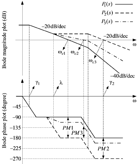
Figure 1: The Bode phase and magnitude plot of the transfer functions given in (5)-(7)

As we know, in dealing with feedback systems non-minimum phase zeros of the process put a limitation on the gain of the controller (recall from the root-locus method that closed-loop poles move toward the open-loop zeros as the gain is increased). On the other hand, the above discussions showed that the gain margin of the feedback system is increased by applying the proposed fractional-order cancellation to the non-minimum phase zero of the process. Hence, it is possible to use controllers with larger gains in the loop when such a cancellation is applied. It turns out that the proposed fractional-order cancellation strategy can partly remove one of the limitations put on the performance of the feedback system by non-minimum phase zeros of the process. Finally, note that although the results of this section are obtained based on studying the Bode plots of two special transfer functions, these are quite general observations and can be easily extended to other cases.

2.2 Effect of the fractional-order unstable pole-zero cancellation on the time-domain undershoot

In this section we show that applying the proposed fractional-order unstable pole-zero cancellation to a non-minimum phase process will reduce the time-domain undershoots in its step response. Note that it can be easily concluded from the previous discussions that the overshoots in the step response of the closed-loop system will be decreased by subjecting the non-minimum phase zero of the process to the proposed fractional-order pole-zero cancellation. More precisely, in Section 2.1 we showed that the proposed method for fractional-order cancellation of non-minimum phase zeros has the property that always increases the phase margin, and as we know increasing the phase margin naturally decreases the time-domain overshoots.

Studying the effect of the proposed cancellation strategy on time-domain undershoots is more complicated. Consider again the process with transfer function $P(s)$ as given in (1). Assuming that the system input, $u(t)$, is equal to the step function and the system is initially at rest, the relative undershoot $r_{us}$ is defined as [16]:

$$r_{us}(y(.))\triangleq-\inf_{t\in(0,\infty)}\left\{\frac{y(t)}{\overline{y}}\right\},$$ (8)

where $\overline{y}$ is equal to the steady-state value of $y(t)$. Clearly, the above definition provides us with a reasonable criterion to compare the undershoot of different systems. The Laplace transforms of $y(t)$ and $u(t)$, respectively denoted as $Y(s)$ and $U(s)$, satisfy the following relation with the process transfer function:

$$Y(s)=\int_{t=0}^{\infty}y(t)e^{-st}dt=P(s)U(s).$$ (9)

Substitution of $s=\lambda$ in (9) and considering the fact that $P(s)$ has a zero at $s=\lambda$ yields:

$$\int_{t=0}^{\infty}y(t)e^{-\lambda t}dt=0.$$ (10)

Suppose that $y(t)$ reaches its steady-state value at $t=T$, that is $y(t)=\overline{y}$ for $t>T$ (clearly, the step response of a LTI system cannot reach its steady-state value at a finite time, but in practice $T$ can be approximated with the settling time of the system step response). Using this assumption equation (10) can be written as

$$\int_{0}^{T}y(t)e^{-\lambda t}dt+\int_{T}^{\infty}\overline{y}e^{-\lambda t}dt=0,$$ (11)

or equivalently,

$$\int_{0}^{T}-\frac{y}{\overline{y}}~{}e^{-\lambda t}dt=\int_{T}^{\infty}e^{-\lambda t}dt=\frac{e^{-\lambda T}}{\lambda}.$$ (12)

Now, according to (8) equation (12) yields

$$\int_{0}^{T}r_{us}e^{-\lambda t}dt\geq\frac{e^{-\lambda T}}{\lambda},$$ (13)

which tunes out

$$r_{us}\geq\frac{1}{e^{\lambda T}-1}.$$ (14)

Equation (14) concludes that the lower bound of the relative undershoot is decreased by increasing the frequency of the non-minimum phase zero, $\lambda$, and/or the settling time, $T$. Both $P(s)$ and $P_{f}(s)$ (as defined in (4)) have a zero at $s=\lambda$ but it is expected that the settling time of the (step) response of a system with transfer function $P_{f}(s)$ be larger than the settling time of the (step) response of a system with transfer function $P(s)$. This statement can easily be concluded from the fact that the settling time of the step response of a system is decreased by increasing its gain crossover frequency (or equivalently, its bandwidth). Since the gain crossover frequency of $P_{f}(s)$ is always smaller than the gain crossover frequency of $P(s)$ it is expected that the response of a system with transfer function $P(s)$ settles down faster than the response of a system with transfer function $P_{f}(s)$. Hence, according to (14) the lower bound on the relative undershoot is decreased by subjecting the non-minimum phase zero of the process to the proposed fractional-order cancellation. Note that although decreasing the lower bound of undershoot does not necessarily mean that the undershoot itself will also be decreased, it shows the potential of the proposed approach for this purpose.

The above result can be extended to feedback systems. The key idea is to note that the bandwidth of the closed-loop system is directly proportional to the gain crossover frequency of the open-loop transfer function. Since applying the fractional-order unstable pole-zero cancellation to the given non-minimum phase process located in a feedback system decreases the gain crossover frequency of the open-loop transfer function, we can conclude that the bandwidth of the closed-loop system is also decreased by performing such a cancellation. As a result, decreasing the bandwidth of the closed-loop system leads to increasing the settling time of the system response to step command and consequently decreasing the lower bound on the relative undershoot.

2.3 Internal-stability analysis of the feedback system containing fractional-order unstable pole-zero cancellation

Previous discussions showed that the proposed strategy for fractional-order cancellation of the non-minimum phase zero of the process can affect some important characteristics of the feedback system. Specially, it was shown that such a cancellation increases the phase and gain margin (and consequently, improves the robustness of system) and potentially can decrease the undershoots in time-domain response. In this section we show that the proposed fractional-order unstable pole-zero cancellation method has the advantage that can be used in feedback systems without leading to internal instability.

Consider the feedback system shown in Fig. 2 where $P(s)$ is the process transfer function defined in (1) and $C(s)$ is the controller. Clearly, the system is internally unstable if $C(s)$ has a pole at $s=\lambda$ (i.e., an unstable pole-zero cancellation occurs in the loop). This fact can be concluded by calculating, e.g., the transfer function from $r$ to $u$, which definitely has an unstable pole at $s=\lambda$. Now, assume that instead of the term $1-s/\lambda$ the denominator of $C(s)$ contains the term $Q_{\lambda,v}(s)=\prod_{k=0}^{\log_{2}(v/2)}\left[1+(s/\lambda)^{2^{k}/v}\right]$, which is equivalent to a fractional-order pole-zero cancellation between $C(s)$ and $P(s)$. In this case, instead of the pole at $s=\lambda$ the transfer function from $r$ to $u$ has poles at the roots of $Q_{\lambda,v}(s)=0$, which are distributed on a Riemann surface. Important point that should be noted here is that the stability of a system with fractional-order characteristic equation $Q_{\lambda,v}(s)=0$ cannot be studied simply by investigating the roots of this equation at the right half-plane of the complex $s$-plane. In fact, according to the stability test of Matignon [17] a system with fractional-order characteristic equation

$$Q_{\lambda,v}(s)=\prod_{k=0}^{\log_{2}(v/2)}\left[1+\left(\frac{s}{\lambda}\right)^{2^{k}/v}\right]=0,$$ (15)

is stable if and only if all roots of the equation $\widetilde{Q}_{\lambda,v}(w)=Q_{\lambda,v}(s)|_{s^{1/v}=w}=0$ lie in the angular sector defined by

$$|\arg(w)|>\frac{\pi}{2v},$$ (16)

in $w$-plane (in other words, $Q_{\lambda,v}(s)=0$ must not have any poles in the closed right half-plane of the first Riemann sheet). It can be easily verified that the roots of $\widetilde{Q}_{\lambda,v}(w)=0$ are as follows:

$$w=e^{j\pi/2^{k}}\lambda^{1/v},\quad k=1,2,\ldots,\log_{2}(v/2).$$ (17)

Since all of these roots are located in the sector of stability defined in (16) we can conclude that the proposed fractional-order pole-zero cancellation method does not change the status of internal stability of the feedback system (stability of all other possible transfer functions in Fig. 2 can be concluded in the same manner). For example, consider the feedback system shown in Fig. 2 and suppose that

$$P(s)=\frac{s-1}{s+2}.$$ (18)

Clearly, in this example $C(s)=1/(s-1)$ leads to internal instability, while assuming

$$C(s)=\frac{1}{Q_{1,2}(s)}=\frac{1}{s^{1/2}+1},$$ (19)

the transfer function from the reference input to control is obtained as

$$\frac{U(s)}{R(s)}=\frac{s+2}{(s^{1/2}+1)(s+s^{1/2}+1)},$$ (20)

which is stable (note that substitution of $s^{1/2}=w$ in the denominator of (20) leads to the characteristic equation $(w+1)(w^{2}+w+1)=0$, all roots of which are located in the sector of stability defined as $|\arg(w)|>\pi/4$).

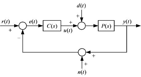
Figure 2: The feedback system under consideration

According to the previous discussions, the structure shown in Fig. 3 can be used for fractional-order unstable zero-pole cancellation and feedback control of the non-minimum phase process with transfer function $P(s)$, which has a non-minimum phase zero at $s=\lambda$. In this structure, the final controller is equal to the series combination of $C(s)$ and $1/Q_{\lambda,v}(s)$. In the proposed method first $Q_{\lambda,v}(s)$ should be determined simply by assigning a suitable integer to $v$ $(v\geq 2)$. The results obtained in Section 2.1 (and presented in Fig. 1) show that the phase-lag of the transfer function $P(s)/Q_{\lambda,v}(s)$ is decreased by increasing the value of $v$, that is the transfer function $P(s)/Q_{\lambda,v}(s)$ becomes less non-minimum phase (and consequently, an easier problem to control) as the value assigned to $v$ is increased. However, simulation results show that in many cases using $v=2$ or $v=4$ leads to satisfactory results.

After determining $Q_{\lambda,v}(s)$ the controller $C(s)$ can be designed using any classical method assuming that the transfer function of process is equal to $P(s)/Q_{\lambda,v}(s)$. Note that since $P(s)/Q_{\lambda,v}(s)$ is a fractional-order transfer function, the controller can be designed in two different ways: One can apply an order-reduction algorithm to $P(s)/Q_{\lambda,v}(s)$ to arrive at an integer-order approximate transfer function and then use a classical controller design algorithm, or one can directly use the methods available to design a controller for the given fractional-order process. Note also that since $P(s)/Q_{\lambda,v}(s)$ has a smaller bandwidth compared to $P(s)$, the controller designed for $P(s)/Q_{\lambda,v}(s)$ naturally applies more control effort compared to the similar controller designed for $P(s)$. A reasonable approach to remove this difficulty is to apply the proposed fractional-order pole-zero cancellation method to both the non-minimum phase zero and a pole of process (an example of this type is studied in Example 3 of Section 3). Finally, note that when $P(s)$ has multiple non-minimum phase zeros, say at $\lambda_{1},\lambda_{2},\ldots,\lambda_{n}$, it is possible to consider a separate fractional-order pole-zero canceller for each non-minimum phase zero.

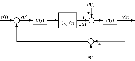
Figure 3: Proposed structure for fractional-order cancellation of the non-minimum phase zero of the process

2.4 Notes on realization of the proposed fractional-order pole-zero canceller

One effective approach to realize the fractional-order pole-zero canceller $Q_{\lambda,v}(s)$ is to approximate it with an integer-order transfer function using an order reduction algorithm (the Matlab function invfreqs is used for this purpose in this paper). Note that although the approximate transfer function obtained by using this method does not guarantee the (partial) cancellation of any non-minimum phase zero or unstable pole of the process, it can be used and will work in practice. The reason for this statement is that the proposed fractional-order pole-zero canceller actually affects the frequency response of the process in a certain manner, and consequently, any other system that applies the similar effects can be used instead. Hence, in practice, we can simply substitute $Q_{\lambda,v}(s)$ with an integer-order transfer function which has almost the same frequency response as $Q_{\lambda,v}(s)$ in the bandwidth of the process.

3 Illustrative examples

Three illustrative examples are presented in this section in order to confirm the results obtained in previous section.

Example 1. The aim of this example is to show that fractional-order cancellation of the non-minimum phase zero of a process leads to decreasing the undershoot and increasing the settling time of its step response. For this purpose consider three processes with the following transfer functions

$$P_{1}(s)=\frac{1-s}{(1+s/2)(1+s/3)},$$ (21)

$$P_{2}(s)=\frac{P_{1}(s)}{1+s^{1/2}}=\frac{1-s^{1/2}}{(1+s/2)(1+s/3)},$$ (22)

$$P_{3}(s)=\frac{P_{1}(s)}{(1+s^{1/2})(1+s^{1/4})}=\frac{1-s^{1/4}}{(1+s/2)(1+s/3)}.$$ (23)

The corresponding unit step responses are shown by $y_{1}(t)$, $y_{2}(t)$, and $y_{3}(t)$ in Fig. 4. As it can also be concluded from (14), it is observed that applying the proposed fractional-order pole-zero cancellation has decreased the undershoot in the unit step response at the cost of increasing the settling time. Since the zero of $P_{3}(s)$ is less non-minimum phase compared to the zero of $P_{2}(s)$, $y_{3}(t)$ exhibits smaller undershoot and larger rise time compared to $y_{2}(t)$.

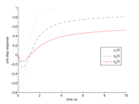
Figure 4: Unit step response of three processes with transfer functions given in (21)-(23), corresponding to Example 1

Example 2. In this example we show that applying the proposed fractional-order pole-zero cancellation strategy to a non-minimum phase process can improve the robust stability of the corresponding feedback system, and consequently make the control problem easier. Consider the feedback system shown in Fig. 3 and assume that

$$P(s)=\frac{4(1-s)}{(s+0.1)(s+4)},$$ (24)

and $C(s)=1$. Figure 5 shows the Bode magnitude and phase plot of $P(s)$, $P(s)/Q_{1,2}(s)$, and $P(s)/Q_{1,4}(s)$. It can be easily verified that in this example $P(s)$, $P(s)/Q_{1,2}(s)$, and $P(s)/Q_{1,4}(s)$ lead to the phase margins $2.7^{\circ}$, $32.7^{\circ}$, and $50.3^{\circ}$, and the gain margins $0.2149$ dB, $4.401$ dB, and $8.958$ dB, respectively. As it is observed the proposed cancellation method has effectively increased the phase and the gain margin.

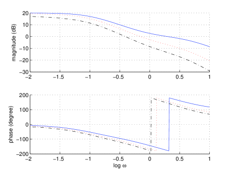
Figure 5: Bode plot of $P(s)$ (solid curve), $P(s)/Q_{1,2}(s)$ (dotted curve), and $P(s)/Q_{1,4}(s)$ (dash-dotted curve), corresponding to Example 2.

Example 3. In this example we show that the proposed fractional-order unstable pole-zero cancellation strategy can enhance the performance of the feedback system by simultaneous decrement of overshoots, undershoots and the control effort. In order to make a fair comparison, we study the behavior of feedback system with and without using the proposed cancellation method, where in both cases $C(s)$ in Fig. 3 is calculated optimally by using the LQG servo-controller design algorithm.

Linearizing the nonlinear equations governing the inverted pendulum shown in Fig. 6 around the unstable equilibrium point at $(x,\theta)=(0,0)$ leads to the following unstable non-minimum phase transfer function [9]:

$$P(s)=\frac{X(s)}{U(s)}=\frac{1}{M}\frac{(s-z)(s+z)}{s^{2}(s-p)(s+p)},$$ (25)

where

$$p=\sqrt{\frac{g}{l}+\frac{mg}{Ml}},\quad z=\sqrt{\frac{g}{l}}.$$ (26)

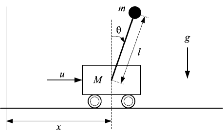
Figure 6: Inverted pendulum, corresponding to Example 3

In the following we design an LQG servo-controller for the linearized process by using and without using the proposed fractional-order unstable pole-zero canceller assuming that $M=m=0.1$ kg, $l=1$ m, and $g=9.8$ $\mathrm{m/s^{2}}$.

First, consider the feedback system shown in Fig. 2. The Matlab function lqg can be used to design a controller for this system such that the cost function:

$$J=E\left\{\lim_{T\rightarrow\infty}\frac{1}{T}\int_{0}^{T}\left([\mathbf{x}^{\mathrm{T}},u]\mathbf{R}\left[\begin{array}[]{c}\mathbf{x}\\ u\\ \end{array}\right]+qe^{2}\right)\mathrm{d}t\right\},$$ (27)

is minimized, where $\mathbf{x}$ is the state vector of process, $u$ is the control applied to process, and $e$ is the tracking error defined as $r-(y+n)$. Without any loss of generality, it is assumed that in the problem under consideration $\mathbf{R}$ is a diagonal matrix of suitable dimension where all non-zero entries are equal to unity, and $q=1$. Moreover, it is assumed that the process noise $w$ (which is not shown in Fig. 2) and measurement noise $n$ are Gaussian white noises with covariance

$$E\left\{\left[\begin{array}[]{c}\mathbf{w}\\ n\\ \end{array}\right][\mathbf{w}^{\mathrm{T}},n]\right\}=\mathbf{M},$$ (28)

where, again without the loss of generality, it is assumed that $\mathbf{M}=\mathrm{diag}[0.1,\ldots,0.1]$. In dealing with the feedback system shown in Fig. 3 the LQG servo-controller can be designed in the same manner assuming that the transfer function of process is equal to $P(s)/Q_{\lambda,v}(s)$.

The simplest possible approach to control a process with the transfer function given in (25) using the feedback system shown in Fig. 3 is to consider $Q_{\lambda,v}(s)$ equal to $s^{1/2}+z^{1/2}$. It can be shown that although this choice can considerably decrease the overshoots and undershoots in the response of feedback system to step command, it will apply more control effort compared to the case such a cancellation is not applied. To remove this difficulty, the fractional-order pole-zero canceller in Fig. 3 (i.e., the box with transfer function $1/Q_{\lambda,v}(s)$) can be substituted with:

$$\frac{Q_{p,2}(s)}{Q_{z,2}(s)}=\frac{s^{1/2}+p^{1/2}}{s^{1/2}+z^{1/2}}.$$ (29)

Note that using the above canceller is equivalent to the half cancellation of both unstable pole and non-minimum phase zero. Now, according to the previous discussions, the LQG servo-controller should be designed for a system with the open-loop transfer function:

$$\frac{(s^{1/2}-z^{1/2})(s+z)}{Ms^{2}\left(s^{1/2}-p^{1/2}\right)(s+p)}.$$ (30)

For this purpose first we should approximate the transfer function given in (30) with an integer-order transfer function by using an order-reduction algorithm. The main reason for working with such an approximate integer-order transfer function is that the standard LQG design algorithm can be applied only to linear processes modelled by integer-order transfer functions. In order to approximate (30) with an integer-order transfer function first we apply the Matlab function invfreqs to the fractional-order transfer function

$$\frac{s^{1/2}-z^{1/2}}{M\left(s^{1/2}-p^{1/2}\right)(s+p)},$$ (31)

and then we add a zero (located at $s=-z$) and two poles (located at $s=0$) to the resulted transfer function. Clearly, it is also possible to apply the invfreqs command directly to (30), but that would lead to less accurate results compared to the proposed approach. The solid and dashed curve in Fig. 7 show the Bode plots of (31) and its approximation, respectively (in this figure the approximation is performed in the frequency range $[10^{-2},10^{2}]$ rad/s, where the degree of the numerator and denominator of the approximating transfer function is considered equal to 6). As it can be observed in Fig. 7 the two plots are in a fair agreement.

The LQG servo-controller is designed for $P(s)$ and $Q_{p,2}(s)P(s)/Q_{z,2}(s)$ (as described above) and the responses of corresponding feedback systems to the unit step command are shown in Fig. 8. In this figure the solid curve shows the cart position when the fractional-order unstable pole-zero canceller given in (29) is applied, and the dotted curve shows the cart position without using such a canceller. This figure clearly shows that the proposed method can effectively improve the response of feedback system by decreasing the overshoots and undershoots.

Note that in order to simulate the feedback system at the presence of fractional-order unstable pole-zero canceller given in (29) we have approximated the canceller with an integer-order transfer function and then we have used it in the connection shown in Fig. 3 (in this example the approximation is performed in the frequency range $[10^{-3},10^{4}]$ rad/s and the order of the numerator and denominator of the approximating transfer function is considered equal to 4). Figure 9 shows the control effort with and without using the fractional-order pole-zero canceller given in (29). Interesting observation is that applying this fractional-order pole-zero canceller also decreases the control effort. More precisely, energy of the control signal with and without using the fractional-order unstable pole-zero canceller is equal to $483.5$ and $693.5$.

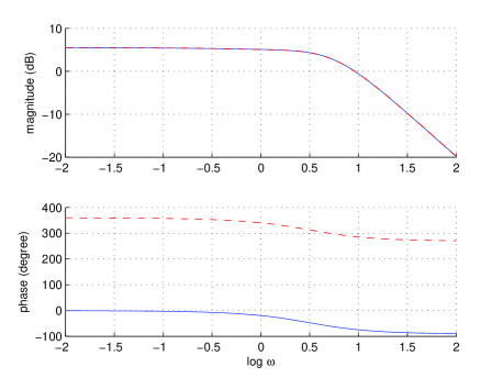
Figure 7: Bode phase and magnitude plot of (31) (solid curve) and its approximation (dashed curve), corresponding to Example 3

Figure 8: Position of the LQG-controlled cart with (solid curve) and without (dotted curve) using the fractional-order unstable pole-zero canceller given in (29), corresponding to Example 3

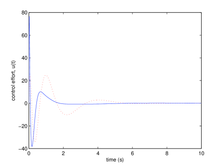
Figure 9: Control effort with (solid curve) and without (dotted curve) using the fractional-order unstable pole-zero canceller given in (29), corresponding to Example 3

4 Conclusion and discussion

In this paper we showed that although the unstable pole-zero cancellation between controller and process is impractical and leads to internal stability, the fractional-order pole-zero cancellation is possible and can be effective. A method for designing fractional-order unstable pole-zero cancellers is proposed and it is specially shown that the proposed method can increase the phase and the gain margin, and consequently, improve the efficiency of the classical controller design algorithm under consideration. Effect of the proposed method on time-domain responses of the non-minimum phase open-loop system is studied and it is shown that it can decrease the overshoots and undershoots in its step response.

There are still many other questions to be answered. For example, the fractional-order unstable pole-zero cancellation strategy can be performed in many other ways. However, it is not exactly known which one is more effective. Moreover, the controller can also be designed using many different methods. It is expected that the proposed fractional-order pole-zero cancellation method be more effective when a certain controller design algorithm is used, but it is not known which one is that. In fact, the proposed approach may also be effective even when the process is minimum phase or stable. These the questions that can be considered as the subject of future studies.

References

- [1] K.J. Åström, R.D. Bell, Drum-boiler dynamics, Automatica, 36 (2000) 363–378.
- [2] J. Hauser, S. Sastry, G. Meyer, Nonlinear control design for slightly non-minimum phase systems: Application to V/STOL aircraft, Automatica, 28(4) (1992) 665–679.
- [3] D.-S. Kwon, W.J. Book, A time-domain inverse dynamic tracking control of a single-link flexible manipulator, Journal of Dynamic Systems, Measurement, and Control, 116 (1994) 193–200.
- [4] C. Kravaris, P. Daoutidis, Nonlinear state feedback control of second-order nonminimum-phase nonlinear systems, Computers and Chemical Engineering, 14(4/5) (1990) 439–449.
- [5] M.M. Seron, J.H. Braslavsky, G.C. Goodwin, Fundamental Limitations in Filtering and Control, New York: Springer-Verlag, 1997.
- [6] M.M. Seron, J.H. Braslavsky, P.V. Kokotovic, D.Q. Mayne, Feedback limitations in nonlinear systems: From Bode integrals to cheap control, IEEE Trans. Automat. Contr. 44 (1999) 829–833.
- [7] L. Qiu, E.J. Davison, Performance limitations of non-minimum phase systems in the servomechanism problem, Automatica, 29 (1993) 337–349.
- [8] R.H. Middleton, Tradeoffs in linear control system design, Automatica, 27(2) (1991) 281–292.
- [9] J.B. Hoagg, D.S. Bernstein, Nonminimum-phase zeros, IEEE Control Systems Magazine, (2007) 45–57.
- [10] J.C. Doyle, B.A. Francis, A.R. Tannenbaum, Feedback Control Theory, New York: Macmillan, 1992.
- [11] T. Kailath, Linear Systems, Englewood Cliffs, NJ: Prentice-Hall, 1980.
- [12] A. Pedro Aguiar, J.P. Hespanha, P.V. Kokotovic, Path-following for nonminimum phase systems removes performance limitations, IEEE Trans. Automat. Contr. 50(2) (2005) 234–239.
- [13] M. Fliess, H. Sira-Ramirez, R. Marquez, Regulation of nonminimum phase outputs: A flatness based approach, in: D. Normand-Cyrot (Ed.), Perspectives in Control-Theory and Applications: A Tribute to Ioan Doré Landau, London, U.K.: Springer-Verlag, 1998, pp. 143 -164.
- [14] S. Al-Hiddabi, N. McClamroch, Tracking and maneuver regulation control for nonlinear nonminimum phase systems: Application to flight control, IEEE Trans. Control Syst. Technol. 10(6) (2002) 780- 792.
- [15] R.A. Silverman, Complex Analysis with Applications, Dover Publications, Inc., New York, 1984.
- [16] K. Lau, R.H. Middleton, J.H. Braslavsky, Undershoot and settling time tradeoffs for nonminimum phase systems, IEEE Trans. Automat. Contr., 48(8) (2003) 1389–1393.
- [17] D. Matignon, Stability properties for generalized fractional differential systems, ESAIM: Proc., 1998, Vol. 5, pp. 145–158.