Extending Partial Representations of Proper and Unit Interval Graphs

Abstract

The recently introduced problem of extending partial interval representations asks, for an interval graph with some intervals pre-drawn by the input, whether the partial representation can be extended to a representation of the entire graph. In this paper, we give a linear-time algorithm for extending proper interval representations and an almost quadratic-time algorithm for extending unit interval representations.

We also introduce the more general problem of bounded representations of unit interval graphs, where the input constrains the positions of some intervals by lower and upper bounds. We show that this problem is NP-complete for disconnected input graphs and give a polynomial-time algorithm for the special class of instances, where the ordering of the connected components of the input graph along the real line is prescribed. This includes the case of partial representation extension.

The hardness result sharply contrasts the recent polynomial-time algorithm for bounded representations of proper interval graphs [Balko et al. ISAAC’13]. So unless $\text{\hbox{\rm P}}=\text{\hbox{\rm NP}}$, proper and unit interval representations have vastly different structure. This explains why partial representation extension problems for these different types of representations require substantially different techniques.

1 Introduction

Geometric intersection graphs, and in particular intersection graphs of objects in the plane, have gained a lot of interest for their practical motivations, algorithmic applications, and interesting theoretical properties. Undoubtedly the oldest and the most studied among them are interval graphs (INT), i.e., intersection graphs of intervals on the real line. They were introduced by Hájos [2] in the 1950’s and the first polynomial-time recognition algorithm appeared already in the early 1960’s [3]. Several linear-time algorithms are known, see [4, 5]. The popularity of this class of graphs is probably best documented by the fact that Web of Knowledge registers over 300 papers with the words “interval graph” in the title. For useful overviews of interval graphs and other intersection-defined classes, see textbooks [6, 7].

Only recently, the following natural generalization of the recognition problem has been considered [8]. The input of the partial representation extension problem consists of a graph and a part of the representation and it asks whether it is possible to extend this partial representation to a representation of the entire graph. Klavík et al. [8] give a quadratic-time algorithm for the class of interval graphs and a cubic-time algorithm for the class of proper interval graphs. Two different linear-time algorithms are given for interval graphs [9, 10]. There are also polynomial-time algorithms for function and permutation graphs [11] as well as for circle graphs [12]. Chordal graph representations as intersection graphs of subtrees of a tree [13] and intersection representations of planar graphs [14] are mostly hard to extend.

A related line of research is the complex of simultaneous representation problems, pioneered by Jampani and Lubiw [15, 16], where one seeks representations of two (or more) input graphs such that vertices shared by the input graphs are represented identically in each of the representations. Although in some cases the problem of finding simultaneous representations generalizes the partial representation extension problem, e.g., for interval graphs [9], this connection does not hold for all graph classes. For example, extending a partial representation of a chordal graph is NP-complete [13], whereas the corresponding simultaneous representation problem is polynomial-time solvable [16]. While a similar reduction as the one from [9] works for proper interval graphs, we are not aware of a direct relation between the corresponding problems for unit interval graphs.

Figure 1: (a) A partial representation which is extendible as a proper interval representation, but not extendible as a unit interval representation. (b) The three structures studied in this paper. The class of proper/unit interval graphs, all proper interval representations and its substructure of all unit interval representations. The denoted mapping $f$ assigns to a representation the graph it represents. The Roberts’ Theorem [17] just states that $f$ restricted to unit interval representations is surjective.

In this paper, we extend the line of research on partial representation extension problems by studying the corresponding problems for proper interval graphs (PROPER INT) and unit interval graphs (UNIT INT). Roberts’ Theorem [17] states $\hbox{\bf\rm PROPER INT}=\hbox{\bf\rm UNIT INT}$. It turns out that specific properties of unit interval representations were never investigated since it is easier to work with combinatorially equivalent proper interval representations. It is already noted in [8] that partial representation extension behaves differently for these two classes; see Figure 1a. This is due to the fact that for proper interval graphs, in whose representations no interval is a proper subset of another interval, the extension problem is essentially topological and can be treated in a purely combinatorial manner. On the other hand, unit interval representations, where all intervals have length one, are inherently geometric, and the corresponding algorithms have to take geometric constraints into account.

It has been observed in other contexts that geometric problems are sometimes more difficult than the corresponding topological problems. For example, the partial drawing extension of planar graphs is linear-time solvable [18] for topological drawing but NP-hard for straight-line drawings [19]. Together with Balko et al. [20], our results show that a generalization of partial representation extension exhibits this behavior already in 1-dimensional geometry. The bounded representation problem is polynomial-time solvable for proper interval graphs [20] and NP-complete for unit interval graphs. From a perspective of representations, this result separates proper and unit interval graphs. We show that, unless $\text{\hbox{\rm P}}=\text{\hbox{\rm NP}}$, the structure of all proper interval representations is significantly different from the structure of all unit interval representations; see Figure 1b.

Next, we formally introduce the problems we study and describe our results.

1.1 Classes and Problems in Consideration

For a graph $G$, an intersection representation $\cal R$ is a collection of sets $\{R_{u}:u\in V(G)\}$ such that $R_{u}\cap R_{v}\neq\emptyset$ if and only if $uv\in E(G)$; so the edges of $G$ are encoded by the intersections of the sets. An intersection-defined class ${\cal C}$ is the class of all graphs having intersecting representations with some specific type of sets $R_{u}$. For example, in an interval representation each $R_{u}$ is a closed interval of the real line. A graph is an interval graph if it has an interval representation.

Studied Classes. We consider two classes of graphs. An interval representation is called proper if no interval is a proper subset of another interval (meaning $R_{u}\subseteq R_{v}$ implies $R_{u}=R_{v}$). An interval representation is called unit if the length of each interval is one. The class of proper interval graphs (PROPER INT) consists of all interval graphs having proper interval representations, whereas the class of unit interval graphs (UNIT INT) consists of all interval graphs having unit interval representations. Clearly, every unit interval representation is also a proper interval representation.

In an interval representation ${\cal R}=\{R_{v}:v\in V\}$, we denote the left and right endpoint of the interval $R_{v}$ by $\ell_{v}$ and $r_{v}$, respectively. For numbered vertices $v_{1},\dots,v_{n}$, we denote these endpoints by $\ell_{i}$ and $r_{i}$. Note that several intervals may share an endpoint in a representation. When we work with multiple representations, we use ${\cal R}^{\prime}$ and $\bar{\cal R}$ for them. Their intervals are denoted by $R^{\prime}_{v}=[\ell^{\prime}_{v},r^{\prime}_{v}]$ and $\bar{R}_{v}=[\bar{\ell}_{v},\bar{r}_{v}]$.

Studied Problems. The recognition problem of a class ${\cal C}$ asks whether an input graph belongs to ${\cal C}$; that is, whether it has a representation by the specific type of sets $R_{u}$. We study two generalizations of this problem: The partial representation extension problem, introduced in [8], and a new problem called the bounded representation problem.

A partial representation ${\cal R}^{\prime}$ of $G$ is a representation of an induced subgraph $G^{\prime}$ of $G$. A vertex in $V(G^{\prime})$ is called pre-drawn. A representation ${\cal R}$ extends ${\cal R}^{\prime}$ if $R_{u}=R^{\prime}_{u}$ for each $u\in V(G^{\prime})$.

Problem: $\textsc{RepExt}({{\cal C}})$ (Partial Representation Extension of ${\cal C}$) Input: A graph $G$ with a partial representation ${\cal R}^{\prime}$. Output: Does $G$ have a representation ${\cal R}$ that extends ${\cal R}^{\prime}$?

Suppose, that we are given two rational numbers $\hbox{\rm{lbound}}(v_{i})$ and $\hbox{\rm{ubound}}(v_{i})$ for each vertex $v_{i}$. A representation ${\cal R}$ is called a bounded representation if $\hbox{\rm{lbound}}(v_{i})\leq\ell_{i}\leq\hbox{\rm{ubound}}(v_{i})$.

Problem: BoundRep (Bounded Representation of UNIT INT) Input: A graph $G$ and two rational numbers $\hbox{\rm{lbound}}(v_{i})$ and $\hbox{\rm{ubound}}(v_{i})$ for each $v_{i}\in V(G)$. Output: Does $G$ have a bounded unit interval representation?

It is easy to see that BoundRep generalizes $\textsc{RepExt}(\hbox{\bf\rm UNIT INT})$ since we can just put $\hbox{\rm{lbound}}(v_{i})=\hbox{\rm{ubound}}(v_{i})=\ell^{\prime}_{i}$ for all pre-drawn vertices, and $\hbox{\rm{lbound}}(v_{i})=-\infty$, $\hbox{\rm{ubound}}(v_{i})=\infty$ for the remaining vertices.

The bounded representation problem can be considered also for interval graphs and proper interval graphs, where the left and right endpoints of the intervals can be restricted individually. A recent paper of Balko et al. [20] proves that this problem is polynomially solvable for these classes. Note that for unit intervals, it suffices to restrict the left endpoint since $r_{i}=\ell_{i}+1$. The complexity for other classes, e.g. circle graphs, circular-arc graphs, permutation graphs, is open.

1.2 Contribution and Outline.

In this paper we present five results. The first is a simple linear-time algorithm for RepExt(PROPER INT), improving over a previous $O(nm)$-time algorithm [8]; it is based on known characterizations, and we present it in Section 3.

Theorem 1.1

$\textsc{RepExt}(\hbox{\bf\rm PROPER INT})$ can be solved in time $\mathcal{O}{}(n+m)$.

We note that this algorithm needs some minor and very natural assumption on the encoding of the input; see Conclusions for details.

Second, in Section 4, we give a reduction from 3-Partition to show that BoundRep is NP-complete for disconnected graphs. The main idea is that prescribed intervals partition the real line into gaps of a fixed width. Integers are encoded in connected components whose unit interval representations require a certain width. By suitably choosing the lower and upper bounds, we enforce that the connected components have to be placed inside the gaps such that they do not overlap.

Theorem 1.2

BoundRep is NP-complete.

Third, in Section 5.1, we give a relatively simple quadratic-time algorithm for the special case of BoundRep where the order of the connected components along the real line is fixed. We formulate this problem as a sequence of linear programs, and we show that each linear program reduces to a shortest-path problem which we solve with the Bellmann-Ford algorithm.

The running time is $O(n^{2}r+nD(r))$, where $r$ is the total encoding length of the bounds in the input, and $D(r)$ is the time required for multiplying or dividing two numbers whose binary representation has length $r$. This is due to the fact that the numbers specifying the upper and lower bounds for the intervals can be quite close to each other, requiring that the corresponding rationals have an encoding that is super-polynomial in $n$. Clearly, two binary numbers whose representations have length $r$ can be added in $O(r)$ time, explaining the term of $O(n^{2}r)$ in the running time. However, using Bellmann-Ford for solving the LP requires also the comparison of rational numbers. To be able to do this efficiently, we convert the rational numbers to a common denominator. Hence, the multiplication cost $D(r)$ enters the running time. The best known algorithm achieves $D(r)=\mathcal{O}{}(r\log r2^{\log^{*}r})$ [22].

Fourth, in Sections 5.2–5.6, we show how to reduce the dependency on $r$ to obtain a running time of $O(n^{2}+nD(r))$, which may be beneficial for instances with bounds that have a long encoding.

Theorem 1.3

BoundRep with a prescribed ordering $\blacktriangleleft$ of the connected components can be solved in time $\mathcal{O}{}(n^{2}+nD(r))$, where $r$ is the size of the input describing bound constraints.

Our algorithm is based on shifting intervals. It starts with some initial representation and creates, by a series of transformations, the so-called left-most representation of the input graph. The algorithm performs $\mathcal{O}{}(n^{2})$ combinatorial iterations, each taking time $\mathcal{O}{}(1)$. The additional time $\mathcal{O}{}(nD(r))$ is used for arithmetic operations with the bounds. The main idea for reducing the running time with respect to the previous approach is to work with short approximations of the involved rational numbers. We compute the precise position of intervals only once, when they reach their final position.

Further, we derive in Sections 4.1, 5.2, and 5.4 many structural results concerning unit interval representations. In particular, we show that all representation of one connected component form a semilattice. We believe that these results might be useful in designing a faster algorithm, attacking other problems, and getting overall better understanding of unit interval representations.

If the number of connected components is small, we can test all possible orderings $\blacktriangleleft$.

Corollary 1.4

For $c$ connected components, BoundRep can be solved in $O(c!(n^{2}+nD(r)))$ time.

Finally, we note that every instance of RepExt(UNIT INT) is an instance of BoundRep. In Section 6, we show how to derive for these special instances a suitable ordering $\blacktriangleleft$ of the connected components, resulting in an efficient algorithm for RepExt(UNIT INT).

Theorem 1.5

$\textsc{RepExt}(\hbox{\bf\rm UNIT INT})$ can be solved in time $\mathcal{O}{}(n^{2}+nD(r))$, where $r$ is the size of the input describing positions of pre-drawn intervals.

All the algorithms described in this paper are also able to certify the extendibility by constructing the required representations.

2 Notation, Preliminaries and Structure

As usual, we reserve $n$ for the number of vertices and $m$ for the number of edges of the graph $G$. We denote the set of vertices by $V(G)$ and the set of edges by $E(G)$. For a vertex $v$, we denote the closed neighborhood of $v$ by $N[v]=\{x:\,vx\in E(G)\}\cup\{v\}$. We also reserve $r$ for the size of the input describing either bound constraints (for the BoundRep problem) or positions of pre-drawn intervals (for $\textsc{RepExt}(\hbox{\bf\rm UNIT INT})$). This value $r$ is for the entire graph $G$, and we use it even when we deal with a single component of $G$. We reserve $c$ for the number of components of $G$ (maximal connected subgraphs of $G$).

(Un)located Components. Unlike the recognition problem, RepExt cannot generally be solved independently for connected components. A connected component $C$ of $G$ is located if it contains at least one pre-drawn interval and unlocated if it contains no pre-drawn interval.

Let ${\cal R}$ be any interval representation. Then for each component $C$, the union $\bigcup_{u\in C}R_{u}$ is a connected segment of the real line, and for different components we get disjoint segments. These segments are ordered from left to right, which gives a linear ordering $\blacktriangleleft$ of the components. So we have $c$ components ordered $C_{1}\blacktriangleleft\cdots\blacktriangleleft C_{c}$.

Structure. The main goal of this paper is to establish Theorem 1.3 and to apply it to solve $\textsc{RepExt}(\hbox{\bf\rm UNIT INT})$. Since this paper contains several other results, the structure might not be completely clear. Now, we try to sketch the story of this paper.

In Section 3, we describe a key structural lemma of Deng et al. [23]. Using this lemma, we give a simple characterization of extendible instances of $\textsc{RepExt}(\hbox{\bf\rm PROPER INT})$, which yields the linear-time algorithm of Theorem 1.1. Also, the reader gets more familiar with the basic difficulties we need to deal with in the case of unit interval graphs.

In Section 4, we show two results for the BoundRep problem. First, we give a polynomial bound on the required resolution of the drawing. So there exists a value $\varepsilon$, which is polynomial in the size of the input, such that there exists a representation where, for every $v_{i}$, the positions $\ell_{i}$ and $r_{i}$ belong to the $\varepsilon$-grid $\{k\varepsilon:k\in\mathbb{Z}\}$. Using this, the required representation can be constructed in this $\varepsilon$-grid. Also, we show that the BoundRep problem is in general NP-complete, which proves Theorem 1.2.

Section 5 is the main section of this paper and it deals with the BoundRep problem with a prescribed ordering $\blacktriangleleft$ of the components. First, we describe an LP-based algorithm for solving this problem that solves $2c$ linear programs. Then we derive some structural results concerning the partially ordered set ${\mathfrak{Rep}}$ of all $\varepsilon$-grid unit interval representations. Using this structure, we conclude the section with a fast combinatorial algorithm for the above linear programs, solving the BoundRep problem in time $\mathcal{O}{}(n^{2}+nD(r))$.

In Section 6, we show using the main theorem that $\textsc{RepExt}(\hbox{\bf\rm UNIT INT})$ can be solved in time $\mathcal{O}{}(n^{2}+nD(r))$. In Conclusions, we deal with the related problem of simultaneous representations and give some open problems.

3 Extending Proper Interval Representations

In this section, we describe how to extend partial representations of proper interval graphs in time $\mathcal{O}{}(m+n)$. We also give a simple characterization of all extendible instances.

Indistinguishable Vertices. Vertices $u$ and $v$ are called indistinguishable if $N[u]=N[v]$. The vertices of $G$ can be partitioned into groups of (pairwise) indistinguishable vertices. Note that indistinguishable vertices may be represented by the same intervals (and this is actually true for general intersection representations). Since indistinguishable vertices are not very interesting from the structural point of view, if the structure of the pre-drawn vertices allows it, we want to prune the graph to keep only one vertex per group.

Suppose that we are given an instance of $\textsc{RepExt}(\hbox{\bf\rm PROPER INT})$. We compute the groups of indistinguishable vertices in time $\mathcal{O}{}(n+m)$ using the algorithm of Rose et al. [24]. Let $u$ and $v$ be two indistinguishable vertices. If $u$ is not pre-drawn, or both vertices are pre-drawn with $R^{\prime}_{u}=R^{\prime}_{v}$, then we remove $u$ from the graph, and in the final constructed representation (if it exists) we put $R_{u}=R_{v}$. For the rest of the section, we shall assume that the input graph and partial representation are pruned. An important property is that for any representation of a pruned graph, it holds that all intervals are pairwise distinct. So if two intervals are pre-drawn in the same position and the corresponding vertices are not indistinguishable, then we stop the algorithm because the partial representation is clearly not extendible.

Left-to-right ordering. Roberts [25] gave the following characterization of proper interval graphs:

Lemma 3.1 (Roberts)

A graph is a proper interval graph if and only if there exists a linear ordering $v_{1}\vartriangleleft v_{2}\vartriangleleft\cdots\vartriangleleft v_{n}$ of its vertices such that the closed neighborhood of every vertex is consecutive.

This linear order $\vartriangleleft$ corresponds to the left-to-right order of the intervals on the real line in some proper interval representation of the graph. In each representation, the order of the left endpoints is exactly the same as the order of the right endpoints, and this order satisfies the condition of Lemma 3.1. For an example of $\vartriangleleft$, see Figure 2.

Figure 2: Two proper interval representations ${\cal R}_{1}$ and ${\cal R}_{2}$ with the left-to-right orderings $v_{1}\vartriangleleft v_{2}\vartriangleleft v_{3}\vartriangleleft v_{4}\vartriangleleft v_{5}\vartriangleleft v_{6}\vartriangleleft v_{7}\vartriangleleft v_{8}$ and $v_{2}\vartriangleleft v_{1}\vartriangleleft v_{3}\vartriangleleft v_{4}\vartriangleleft v_{5}\vartriangleleft v_{7}\vartriangleleft v_{6}\vartriangleleft v_{8}$.

How many different orderings $\vartriangleleft$ can a proper interval graph admit? In the case of a general unpruned graph possibly many, but all of them have a very simple structure. In Figure 2, the graph contains two groups $\{v_{1},v_{2},v_{3}\}$ and $\{v_{6},v_{7}\}$. The vertices of each group have to appear consecutively in the ordering $\vartriangleleft$ and may be reordered arbitrarily. Deng et al. [23] proved the following:

Lemma 3.2 (Deng et al.)

For a connected (unpruned) proper interval graph, the ordering $\vartriangleleft$ satisfying the condition of Lemma 3.1 is uniquely determined up to local reordering of groups of indistinguishable vertices and complete reversal.

This lemma is key for partial representation extension of proper interval graphs. Essentially, we just have to deal with a unique ordering (and its reversal) and match the partial representation on it. Notice that in a pruned graph, if two vertices are indistinguishable, then their order is prescribed by the partial representation.

We want to construct a partial ordering $<$ which is a simple representation of all orderings $\vartriangleleft$ from Lemma 3.1. There exists a proper interval representation with an ordering $\vartriangleleft$ if and only if $\vartriangleleft$ extends either $<$ or its reversal. According to Lemma 3.2, $<$ can be constructed by taking an arbitrary ordering $\vartriangleleft$ and making indistinguishable vertices incomparable. For the graph in Figure 2, we get

$$(v_{1},v_{2},v_{3})<v_{4}<v_{5}<(v_{6},v_{7})<v_{8},$$

where groups of indistinguishable vertices are put in brackets. This ordering is unique up to reversal and can be constructed in time $\mathcal{O}{}(n+m)$ [26].

Characterization of Extendible Instances. We give a simple characterization of the partial representation instances that are extendible. We start with connected instances. Let $G$ be a pruned proper interval graph and ${\cal R}^{\prime}$ be a partial representation of its induced subgraph $G^{\prime}$. Then intervals in ${\cal R}^{\prime}$ are in some left-to-right ordering $<^{{\cal R}^{\prime}}$. (Recall that the pre-drawn intervals are pairwise distinct.)

Lemma 3.3

The partial representation ${\cal R}^{\prime}$ of a connected graph $G$ is extendible if and only if there exists a linear ordering $\vartriangleleft$ of $V(G)$ such that:

1. The ordering $\vartriangleleft$ extends $<^{{\cal R}^{\prime}}$, and either $<$ or its reversal.

2. Let $R^{\prime}_{u}$ and $R^{\prime}_{v}$ be two pre-drawn touching intervals, i.e., $r_{u}=\ell_{v}$, and let $w$ be any vertex distinct from $u$ and $v$. If $uw\in E(G)$, then $w\vartriangleleft v$, and if $vw\in E(G)$, then $u\vartriangleleft w$.

Proof 1

If there exists a representation ${\cal R}$ extending ${\cal R}^{\prime}$, then it is in some left-to-right ordering $\vartriangleleft$. Clearly, the pre-drawn intervals are placed the same, so $\vartriangleleft$ has to extend $<^{{\cal R}^{\prime}}$. According to Lemma 3.2, $\vartriangleleft$ extends $<$ or its reversal. As for (2), clearly $v$ has to be the right-most neighbor of $u$ in ${\cal R}$: If $R_{w}$ is on the right of $R_{v}$, it would not intersect $R_{u}$. Similarly, $u$ is the left-most neighbor of $v$.

Conversely, let $v_{1}\vartriangleleft\cdots\vartriangleleft v_{n}$ be an ordering from the statement of the lemma. We construct a representation ${\cal R}$ extending ${\cal R}^{\prime}$ as follows. We compute a common linear ordering $\lessdot$ of the left and right endpoints from left-to-right. We start with the ordering $\ell_{1}\lessdot\cdots\lessdot\ell_{n}$, into which we insert the right endpoints $r_{1},\dots,r_{n}$ one-by-one. For vertex $v_{i}$, let $v_{j}$ be its right-most neighbor in the ordering $\vartriangleleft$. Then, we place $r_{i}$ right before $\ell_{j+1}$ (if $j<n$, otherwise we append $r_{i}$ to the end of the ordering).

This left-to-right common order $\lessdot$ is uniquely determined by $\vartriangleleft$. Since $\vartriangleleft$ extends $<^{{\cal R}^{\prime}}$, it is compatible with the partial representation (the pre-drawn endpoints are ordered as in $\lessdot$). To construct the representation, we just place the non-pre-drawn endpoints equidistantly into the gaps between neighboring pre-drawn endpoints (or to the left or right of ${\cal R}^{\prime}$). It is important that, if two pre-drawn endpoints $\ell_{i}$ and $r_{j}$ share their position, then according to condition (2) there is no endpoint placed in between of $\ell_{i}$ and $r_{j}$ in $\lessdot$ (otherwise one of the two implications would not hold, depending whether a left endpoint is intersected in between, or a right one). See Figure 3 for an example.

Figure 3: Representation of a component with order $1\vartriangleleft 2\vartriangleleft 3\vartriangleleft 4\vartriangleleft 5\vartriangleleft 6$. First, we compute the common order of the left and right endpoints: $\ell_{1}\lessdot\ell_{2}\lessdot r_{1}\lessdot\ell_{3}\lessdot\ell_{4}\lessdot r_{2}\lessdot r_{3}\lessdot\ell_{5}\lessdot r_{4}\lessdot\ell_{6}\lessdot r_{5}\lessdot r_{6}$. The endpoints of the pre-drawn intervals split the segment into several subsegments. We place the remaining endpoints in this order and, within every subsegment, distributed equidistantly.

We argue correctness of the constructed representation ${\cal R}$. First, it extends ${\cal R}^{\prime}$, since the pre-drawn intervals are not modified. Second, it is a correct interval representation: Let $v_{i}$ and $v_{j}$ be two vertices with $v_{i}\vartriangleleft v_{j}$, and let $v_{k}$ be the right-most neighbor of $v_{i}$ in $\vartriangleleft$. If $v_{i}v_{j}\in E(G)$, then $\ell_{i}\lessdot\ell_{k}\lessdot r_{i}$ and, by consecutivity of $N[u]$ in $\vartriangleleft$, we have $\ell_{j}\lessdot\ell_{k}$. Therefore, $R_{v_{i}}$ and $R_{v_{j}}$ intersect. If $v_{i}v_{j}\notin E(G)$ and $v_{j}\neq v_{k+1}$, then $r_{i}\lessdot\ell_{k+1}\lessdot\ell_{j}$, so $R_{v_{i}}$ and $R_{v_{j}}$ do not intersect. If $v_{i}v_{j}\notin E(G)$ and $v_{j}=v_{k+1}$, then $r_{i}\lessdot\ell_{k+1}$ and $R_{v_{i}}$ and $R_{v_{j}}$ do not intersect. Finally, we argue that ${\cal R}$ is a proper interval representation. In $\lessdot$ the order of the left endpoints is the same as the order of the right-endpoints, since $r_{i+1}$ is always placed on the right of $r_{i}$ in $\lessdot$.

We conclude that the representation ${\cal R}$ can be made small enough to fit into any open segment of the real line that contains all pre-drawn intervals.

Now, we are ready to characterize general solvable instances.

Lemma 3.4

A partial representation ${\cal R}^{\prime}$ of a graph $G$ is extendible if and only if

1. for each component $C$, the partial representation ${\cal R}^{\prime}_{C}$ consisting of the pre-drawn intervals in $C$ is extendible, and

2. pre-drawn vertices of each component are consecutive in $<^{{\cal R}^{\prime}}$.

Proof 2

The necessity of (1) is clear. For (2), if some component $C$ would not have its pre-drawn vertices consecutive in $<^{{\cal R}^{\prime}}$, then $\bigcup_{u\in C}R_{u}$ would not be a connected segment of the real line (contradicting existence of $\blacktriangleleft$ from Preliminaries).

Now, if the instance satisfies both conditions we can construct a correct representation ${\cal R}$ extending ${\cal R}^{\prime}$ as follows. Using (2), the located components are ordered from left to right, and we assign pairwise disjoint open segments containing all their pre-drawn intervals (there is a non-empty gap between located components we can use). To unlocated components, we assign pairwise disjoint open segments to the right of the right-most located component. See Figure 4. For each component, we construct a representation in its open segment, using the construction in the proof of Lemma 3.3.

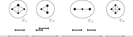
Figure 4: An example of a graph with four components $C_{1},\dots,C_{4}$. The pre-drawn intervals give the order of the located components $C_{1}\blacktriangleleft C_{2}\blacktriangleleft C_{3}$. The non-located component $C_{4}$ is placed to the right. For each component, we reserve some segment in which we construct the representation.

We are ready to prove that $\textsc{RepExt}(\hbox{\bf\rm PROPER INT})$ can be solved in time $\mathcal{O}{}(n+m)$:

Proof 3 (Theorem 1.1)

We just use the characterization by Lemma 3.4, of which the conditions (1) and (2) can be easily checked in time $\mathcal{O}{}(n+m)$. For Lemma 3.3, we check for each component both constraints (1) and (2). To check (2), we compute for $<$ and its reversal the unique orderings $\vartriangleleft$. We test for each of them whether each touching pair of pre-drawn intervals is placed in $\vartriangleleft$ according to (2).

If necessary, a representation ${\cal R}$ can be constructed in the same running time since the proofs of Lemmas 3.3 and 3.4 are constructive.

4 Bounded Representations of Unit Interval Graphs

In this section, we deal with bounded representations. An input of BoundRep consists of a graph $G$ and, for each vertex $v_{i}$, a lower bound $\hbox{\rm{lbound}}(v_{i})$ and an upper bound $\hbox{\rm{ubound}}(v_{i})$. (We allow $\hbox{\rm{lbound}}(v_{i})=-\infty$ and $\hbox{\rm{ubound}}(v_{i})=+\infty$.) The problem asks whether there exists a unit interval representation ${\cal R}$ of $G$ such that $\hbox{\rm{lbound}}(v_{i})\leq\ell_{i}\leq\hbox{\rm{ubound}}(v_{i})$ for each interval $v_{i}$. Such a representation is called a bounded representation.

Since unit interval representations are proper interval representations, all properties of proper interval representations described in Section 3 hold, in particular the properties of orderings $\vartriangleleft$ and $<$.

4.1 Representations in $\varepsilon$-grids

Endpoints of intervals can be positioned at arbitrary real numbers. For the purpose of the algorithm, we want to work with representations drawn in limited resolution. For a given instance of the bounded representation problem, we want to find a lower bound for the required resolution such that this instance is solvable if and only if it is solvable in this limited resolution.

More precisely, we want to represent all intervals so that their endpoints correspond to points on some grid. For a value $\varepsilon={1\over K}>0$, where $K$ is an integer, the $\varepsilon$-grid is the set of points $\{k\varepsilon:k\in\mathbb{Z}\}$. For a given instance of BoundRep, we ask which value of $\varepsilon$ ensures that we can construct a representation having all endpoints on the $\varepsilon$-grid. So the value of $\varepsilon$ is the resolution of the drawing.

If there are no bounds, every unit interval graph has a representation in the grid of size $1\over n$ [26]. In the case of BoundRep, the size of the grid has to depend on the values of the bounds. Consider all values $\hbox{\rm{lbound}}(v_{i})$ and $\hbox{\rm{ubound}}(v_{i})$ distinct from $\pm\infty$, and express them as irreducible fractions ${p_{1}\over q_{1}},{p_{2}\over q_{2}},\cdots,{p_{b}\over q_{b}}$. Then we define:

$$\varepsilon^{\prime}:={1\over\text{lcm}(q_{1},q_{2},\dots,q_{b})},\qquad{\text{and}}\qquad\varepsilon:={\varepsilon^{\prime}\over n},$$ (1)

where $\text{lcm}(q_{1},q_{2},\dots,q_{b})$ denotes the least common multiple of $q_{1},\dots,q_{b}$. It is important that the size of this $\varepsilon$ written in binary is $\mathcal{O}{}(r)$. We show that the $\varepsilon$-grid is sufficient to construct a bounded representation:

Lemma 4.1

If there exists a bounded representation ${\cal R}^{\prime}$ for an input of the problem BoundRep, there exists a bounded representation ${\cal R}$ in which all intervals have endpoints on the $\varepsilon$-grid, where $\varepsilon$ is defined by (1).

Proof 4

We construct an $\varepsilon$-grid representation ${\cal R}$ from ${\cal R}^{\prime}$ in two steps. First, we shift intervals to the left, and then we shift intervals slightly back to the right. For every interval $v_{i}$, the sizes of the left and right shifts are denoted by $\text{LS}(v_{i})$ and $\text{RS}(v_{i})$ respectively. The shifting process is shown in Figure 5.

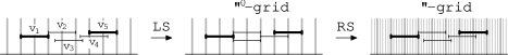
Figure 5: In the first step, we shift intervals to the left to the $\varepsilon^{\prime}$-grid. The left shifts of $v_{1},\dots,v_{5}$ are $(0,0,{1\over 2}\varepsilon^{\prime},{1\over 3}\varepsilon^{\prime},0)$. In the second step, we shift to the right in the refined $\varepsilon$-grid. Right shifts have the same relative order as left shifts: $(0,0,2\varepsilon,\varepsilon,0)$.

In the first step, we consider the $\varepsilon^{\prime}$-grid and shift all the intervals to the left to the closest grid-point (we do not shift an interval if its endpoints are already on the grid). Original intersections are kept by this shifting, since if $x$ and $y$ are two endpoints satisfying $x\leq y$ before the left-shift, then $x\leq y$ also holds after the left-shift. So if $v_{i}v_{j}\in E$ and $\ell_{i}\leq\ell_{j}\leq r_{i}$ before the shift, then these inequalities are preserved by the shifting. On the other hand, we may introduce additional intersections by shifting two non-intersecting intervals to each other. In this case, after the left-shift, the intervals only touch; for an example, see vertices $v_{2}$ and $v_{4}$ in Figure 5.

The second step shifts the intervals to the right in the refined $\varepsilon$-grid to remove the additional intersections created by the first step. The right-shift is a mapping

$$\text{RS}:\{v_{1},\dots,v_{n}\}\to\{0,\varepsilon,2\varepsilon,\dots,(n-1)\varepsilon\}$$

having the right-shift property: For all pairs $(v_{i},v_{j})$ with $r_{i}=\ell_{j}$, $\text{RS}(v_{i})\geq\text{RS}(v_{j})$ if and only if $v_{i}v_{j}\in E$. So the right-shift property ensures that RS fixes wrongly represented touching pairs created by LS.

To construct such a mapping RS, notice that if we relax the image of RS to $[0,\varepsilon^{\prime})$, the reversal of LS would have the right-shift property, since it produces the original correct representation ${\cal R}^{\prime}$. But the right-shift property depends only on the relative order of the shifts and not on the precise values. Therefore, we can construct RS from the reversal of LS by keeping the shifts in the same relative order. If $\text{LS}(v_{i})$ is one of the $k$th smallest shifts, we set $\text{RS}(v_{i})=(k-1)\varepsilon$. See Figure 5.

We finally argue that these shifts produce a correct $\varepsilon$-grid representation. The right-shift does not create additional intersections: After LS non-intersecting pairs are at distance at least $\varepsilon^{\prime}=n\varepsilon$, and by RS they can get closer by at most $(n-1)\varepsilon$. Also, if after LS two intervals overlap by at least $\varepsilon^{\prime}$, their intersection is not removed by RS. The only intersections which are modified by RS are touching pairs of intervals $(v_{i},v_{j})$ having $r_{i}=\ell_{j}$ after LS. The mapping RS shifts these pairs correctly according to the edges of the graph.

Next we look at the bound constraints. If, before the shifting, $v_{i}$ was satisfying $\ell_{i}\geq\hbox{\rm{lbound}}(v_{i})$, then this is also satisfied after $\text{LS}(v_{i})$ since the $\varepsilon^{\prime}$-grid contains the value $\hbox{\rm{lbound}}(v_{i})$. Obviously, the inequality is not broken after $\text{RS}(v_{i})$. As for the upper bound, if $\text{LS}(v_{i})=0$ and $\text{RS}(v_{i})=0$, then the bound is trivially satisfied. Otherwise, after $\text{LS}(v_{i})$ we have $\ell_{i}\leq\hbox{\rm{ubound}}(v_{i})-\varepsilon^{\prime}$, so the upper bound still holds after $\text{RS}(v_{i})$.

Additionally, Lemma 4.1 shows that it is always possible to construct an $\varepsilon$-grid representation having the same topology as the original representation, in the sense that overlapping pairs of intervals keep overlapping, and touching pairs of intervals keep touching. Also notice that both representations ${\cal R}$ and ${\cal R}^{\prime}$ have the same order of the intervals.

In the standard unit interval graph representation problem, no bounds on the positions of the intervals are given, and we get $\varepsilon^{\prime}=1$ and $\varepsilon={1\over n}$. Lemma 4.1 proves in a particularly clean way that the grid of size $1\over n$ is sufficient to construct unrestricted representations of unit interval graphs. Corneil et al. [26] show how to construct this representation directly from the ordering $<$, whereas we use some given representation to construct an $\varepsilon$-grid representation.

4.2 Hardness of BoundRep

In this subsection we focus on hardness of bounded representations of unit interval graphs. We prove Theorem 1.2 stating that BoundRep is NP-complete.

We reduce the problem from 3-Partition. An input of 3-Partition consists of natural numbers $k$, $M$, and $A_{1},\dots,A_{3k}$ such that ${M\over 4}<A_{i}<{M\over 2}$ for all $i$, and $\sum A_{i}=kM$. The question is whether it is possible to partition the numbers $A_{i}$ into $k$ triples such that each triple sums to exactly $M$. This problem is known to be strongly NP-complete (even if all numbers have polynomial sizes) [27].

Proof 5 (Theorem 1.2)

According to Lemma 4.1, if there exists a representation satisfying the bound constraints, then there also exists an $\varepsilon$-grid representation with this property. Since the length of $\varepsilon$ given by (1), written in binary, is polynomial in the size of the input, all endpoints can be placed in polynomially-long positions. Thus we can guess the bounded representation and the problem belongs to NP.

Let us next prove that the problem is NP-hard. For a given input of 3-Partition, we construct the following unit interval graph $G$. For each number $A_{i}$, we add a path $P_{2A_{i}}$ (of length $2A_{i}-1$) into $G$ as a separate component. For all vertices $x$ in these paths, we set bounds

$$\hbox{\rm{lbound}}(x)=1\qquad\text{and}\qquad\hbox{\rm{ubound}}(x)=k\cdot(M+2).$$

In addition, we add $k+1$ independent vertices $v_{0},v_{1},\dots,v_{k}$, and make their positions in the representation fixed:

$$\hbox{\rm{lbound}}(v_{i})=\hbox{\rm{ubound}}(v_{i})=i\cdot(M+2).$$

See Figure 6 for an illustration of the reduction. Clearly, the reduction is polynomial.

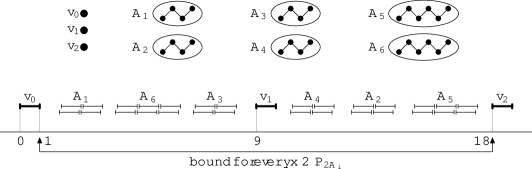
Figure 6: We consider the following input for 3-Partition: $k=2$, $M=7$, $A_{1}=A_{2}=A_{3}=A_{4}=2$ and $A_{5}=A_{6}=3$. The associated unit interval graph is depicted on top, and at the bottom we find one of its correct bounded representations, giving 3-partitioning $\{A_{1},A_{3},A_{6}\}$ and $\{A_{2},A_{4},A_{5}\}$.

We now argue that the bounded representation problem is solvable if and only if the given input of 3-Partition is solvable. Suppose first that the bounded representation problem admits a solution. There are $k$ gaps between the fixed intervals $v_{0},\dots,v_{k}$ each of which has space less than $M+1$. (The length of the gap is $M+1$ but the endpoints are taken by $v_{i}$ and $v_{i+1}$.) The bounds of the paths force their representations to be inside these gaps, and each path lives in exactly one gap. Hence the representation induces a partition of the paths.

Now, the path $P_{2A_{i}}$ needs space at least $A_{i}$ in every representation since it has an independent set of the size $A_{i}$. The representations of the paths may not overlap and the space in each gap is less than $M+1$, hence the sum of all $A_{i}$’s in each part is at most $M$. Since the total sum of $A_{i}$’s is exactly $kM$, the sum in each part has to be $M$. Thus the obtained partition solves the 3-Partition problem.

Conversely, every solution of 3-Partition can be realized in this way.

5 Bounded Representations of Unit Interval Graphs with Prescribed Ordering

In this section, we deal with the BoundRep problem when a fixed ordering $\blacktriangleleft$ of the components is prescribed. First we solve the problem using linear programming. Then we describe additional structure of bounded representations, and using this structure we construct an almost quadratic-time algorithm that solves the linear programs.

5.1 LP Approach for BoundRep

According to Lemma 3.2, each component of $G$ can be represented in at most two different ways, up to local reordering of groups of indistinguishable vertices. Unlike the case of proper interval graphs, we cannot arbitrarily choose one of the orderings, since neighboring components restrict each other’s space. For example, only one of the two orderings for the component $C_{1}$ in Figure 7 makes a representation of $C_{2}$ possible.

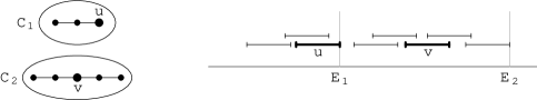
Figure 7: The positions of the vertices $u$ and $v$ are fixed by the bound constraints. The component $C_{1}$ can only be represented with $u$ being the right-most interval, since otherwise $C_{1}$ would block space for the component $C_{2}$.

In the algorithm, we process components $C_{1}\blacktriangleleft C_{2}\blacktriangleleft\cdots\blacktriangleleft C_{c}$ from left to right and construct representations for them. When we process a component $C_{t}$, we want to represent it on the right of the previous component $C_{t-1}$, and we want to push the representation of $C_{t}$ as far to the left as possible, leaving as much space for $C_{t+1},\dots,C_{c}$ as possible.

Now, we describe in details, how we process a component $C_{t}$. We calculate by the algorithm of Corneil et al. the partial ordering $<$ described in Section 3 and its reversal. The elements that are incomparable by these partial orderings are vertices of the same group of indistinguishable vertices. For these vertices, the following holds:

Lemma 5.1

Suppose there exists some bounded representation ${\cal R}$. Then there exists a bounded representation ${\cal R}^{\prime}$ such that, for every indistinguishable pair $v_{i}$ and $v_{j}$ satisfying $\hbox{\rm{lbound}}(v_{i})\leq\hbox{\rm{lbound}}(v_{j})$, it holds that $\ell^{\prime}_{i}\leq\ell^{\prime}_{j}$.

Proof 6

Given a representation ${\cal R}$, we call a pair $(v_{i},v_{j})$ bad if $v_{i}$ and $v_{j}$ are indistinguishable, $\hbox{\rm{lbound}}(v_{i})\leq\hbox{\rm{lbound}}(v_{j})$ and $\ell_{i}>\ell_{j}$. We describe a process which iteratively constructs ${\cal R}^{\prime}$ from ${\cal R}$, by constructing a sequence of representations ${\cal R}={\cal R}_{0},{\cal R}_{1},\dots,{\cal R}_{k}={\cal R}^{\prime}$, where the positions in a representation ${\cal R}_{s}$ are denoted by $\ell^{s}_{i}$’s.

In each step $s$, we create ${\cal R}_{s}$ from ${\cal R}_{s-1}$ by fixing one bad pair $(v_{i},v_{j})$: we set $\ell^{s}_{i}=\ell^{s-1}_{j}$ and the rest of the representation remains the same. Since $v_{i}$ and $v_{j}$ are indistinguishable and ${\cal R}_{s-1}$ is correct, the obtained ${\cal R}_{s}$ is a representation. Regarding bound constraints,

$$\hbox{\rm{lbound}}(v_{i})\leq\hbox{\rm{lbound}}(v_{j})\leq\ell^{s-1}_{j}=\ell^{s}_{i}<\ell^{s-1}_{i}\leq\hbox{\rm{ubound}}(v_{i}),$$

so the bounds of $v_{i}$ are satisfied.

Now, in each ${\cal R}_{s}$ the set of all left endpoints is a subset of the set of all left endpoints of ${\cal R}$. In each step, we move one left-endpoint to the left, so each endpoint is moved at most $n-1$ times. Hence the process terminates after $\mathcal{O}{}(n^{2})$ iterations and produces a representation ${\cal R}^{\prime}$ without bad pairs as requested.

For $<$ and its reversal, we use Lemma 5.1 to construct linear orderings $\vartriangleleft$: If $v_{i}$ and $v_{j}$ belong to the same group of indistinguishable vertices and $\hbox{\rm{lbound}}(v_{i})<\hbox{\rm{lbound}}(v_{j})$, then $v_{i}\vartriangleleft v_{j}$. If $\hbox{\rm{lbound}}(v_{i})=\hbox{\rm{lbound}}(v_{j})$, we choose any order $\vartriangleleft$ between $v_{i}$ and $v_{j}$.

We obtain two total orderings $\vartriangleleft$, and we solve a linear program for each of them. Let $v_{1}\vartriangleleft v_{2}\vartriangleleft\cdots\vartriangleleft v_{k}$ be one of these orderings. We denote the right-most endpoint of a representation of a component $C_{t}$ by $E_{t}$. Additionally, we define $E_{0}=-\infty$. Let $\varepsilon$ be defined as in (1). We modify all lower bounds by putting $\hbox{\rm{lbound}}(v_{i})=\max\bigl{\{}\hbox{\rm{lbound}}(v_{i}),E_{t-1}+\varepsilon\bigr{\}}$ for every interval $v_{i}$, which forces the representation of $C_{t}$ to be on the right of the previously constructed representation of $C_{t-1}$. The linear program has variables $\ell_{1},\dots,\ell_{k}$, and it minimizes the value of $E_{t}$. We solve:

Minimize: $$E_{t}:\! =\ell_{k}+1,\qquad\ \,$$

subject to: $$\ell_{i} \leq\ell_{i+1}, \forall i=1,\dots,k-1,$$ (2)

$$\ell_{i} \geq\hbox{\rm{lbound}}(v_{i}), \forall i=1,\dots,k,$$ (3)

$$\ell_{i} \leq\hbox{\rm{ubound}}(v_{i}), \forall i=1,\dots,k,$$ (4)

$$\ell_{i} \geq\ell_{j}-1, \forall v_{i}v_{j}\in E(G),v_{i}\vartriangleleft v_{j},$$ (5)

$$\ell_{i}+\varepsilon \leq\ell_{j}-1, \forall v_{i}v_{j}\notin E(G),v_{i}\vartriangleleft v_{j}.$$ (6)

We solve the same linear program for the other ordering of the vertices of $C_{t}$. If none of the two programs is feasible, we report that no bounded representation exists. If exactly one of them is feasible, we keep the values obtained for $\ell_{1},\dots,\ell_{k}$ and $E_{t}$, and process the next component $C_{t+1}$. If the two problems are feasible, we keep the solution in which the value of $E_{t}$ is smaller, and process $C_{t+1}$.

Lemma 5.2

Let the representation of $C_{t-1}$ be fixed. Every bounded $\varepsilon$-grid representation of the component $C_{t}$ with the left-to-right order $v_{1}\vartriangleleft\cdots\vartriangleleft v_{k}$ which is on the right of the representation of $C_{t-1}$ satisfies constraints (3)–(6).

Proof 7

Constraints of types (3) and (4) are satisfied, since the representation is bounded and on the right of $C_{t-1}$. Constraints of type (5) correspond to a correct representation of intersecting pairs of intervals. The non-intersecting pairs of an $\varepsilon$-grid representation are at distance at least $\varepsilon$, which makes constraints of type (6) satisfied.

Now, we are ready to show:

Proposition 5.3

The BoundRep problem with prescribed $\blacktriangleleft$ can be solved in polynomial time.

Proof 8

Concerning the running time, it depends polynomially on the sizes of $n$ and $\varepsilon$, which are polynomial in the size of the input $r$. It remains to show correctness.

Suppose that the algorithm returns a candidate for a bounded representation. The formulation of the linear program ensures that it is a correct representation: Constraints of type (2) make the representation respect $\vartriangleleft$. Constraints of type (3) and (4) enforce that the given lower and upper bounds for the positions of the intervals are satisfied, force the prescribed ordering $\blacktriangleleft$ on the representation of $G$, and force the drawings of the distinct components to be disjoint. Finally, constraints of type (2), (5) and (6) make the drawing of the vertices of a particular component $C_{t}$ to be a correct representation.

Suppose next that a bounded representation exists. According to Lemma 4.1 and Lemma 5.1, there also exists an $\varepsilon$-grid bounded representation ${\cal R}^{\prime}$ having the order in the indistinguishable groups as defined above. So for each component $C_{t}$, one of the two orderings $\vartriangleleft$ constructed for the linear programs agrees with the left-to-right order of $C_{t}$ in ${\cal R}^{\prime}$.

We want to show that the representation of each component $C_{t}$ in ${\cal R}^{\prime}$ gives a solution to one of the two linear programs associated to $C_{t}$. We denote by $E^{\prime}_{t}$ the value of $E_{t}$ in the representation ${\cal R}^{\prime}$, and by $E^{\min}_{t}$ the value of $E_{t}$ obtained by the algorithm after solving the two linear programming problems associated to $C_{t}$. We show by induction on $t$ that $E^{\min}_{t}\leq E^{\prime}_{t}$, which specifically implies that $E^{\min}_{t}$ exists and at least one of the linear programs for $C_{t}$ is solvable.

We start with $C_{1}$. As argued above, the left-to-right order in ${\cal R}^{\prime}$ agrees with one of the orderings $\vartriangleleft$, so the representation of $C_{1}$ satisfies the constraints (2). Since $E_{0}=-\infty$, the lower bounds are not modified. By Lemma 5.2, the rest of the constraints are also satisfied. Thus the representation of $C_{1}$ gives a feasible solution for the program and gives $E^{\min}_{1}\leq E^{\prime}_{1}$.

Assume now that, for some $C_{t}$ with $t\geq 1$, at least one of the two linear programming problems associated to $C_{t}$ admits a solution, and from induction hypothesis we have $E^{\min}_{t}\leq E^{\prime}_{t}$. In ${\cal R}^{\prime}$, two neighboring components are represented at distance at least $\varepsilon$. Therefore for every vertex $v_{i}$ of $C_{t+1}$, it holds $\ell_{i}\geq E^{\prime}_{t}+\varepsilon\geq E^{\min}_{t}+\varepsilon$, so the modification of the lower bound constraints is satisfied by ${\cal R}^{\prime}$. Similarly as above using Lemma 5.2, the representation of $C_{t+1}$ in ${\cal R}^{\prime}$ satisfies the remaining constraints. It gives some solution to one of the programs and we get $E^{\min}_{t+1}\leq E^{\prime}_{t+1}$.

In summary, if there exists a bounded representation, for each component $C_{t}$ at least one of the two linear programming problems associated to $C_{t}$ admits a solution. Therefore, the algorithm returns a correct bounded representation ${\cal R}$ (as discussed in the beginning of the proof). We note that ${\cal R}$ does not have to be an $\varepsilon$-grid representation since the linear program just states that non-intersecting intervals are at distance at least $\varepsilon$. To construct an $\varepsilon$-grid representation if necessary, we can proceed as in the proof of Lemma 4.1.

We note that it is possible to reduce the number of constraints of the linear program from $\mathcal{O}{}(k^{2})$ to $\mathcal{O}{}(k)$, since neighbors of each $v_{i}$ appear according to Lemma 3.1 consecutively in $\vartriangleleft$. Using the ordering constraints (2), we can replace constraints (5) and (6) by a linear number of constraints as follows. For each $v_{j}$, there are two cases. If $v_{j}$ is adjacent to all vertices $v_{i}$ such that $v_{i}\vartriangleleft v_{j}$, then we only state the constraint (5) for $v_{1}$ and $v_{j}$. Otherwise, let $v_{i}$ be the rightmost vertex such that $v_{i}\vartriangleleft v_{j}$ and $v_{i}v_{j}\notin E$. Then we only state the constraint (5) for $v_{i+1}$ and $v_{j}$, and the constraint (6) for $v_{i}$ and $v_{j}$. This is equivalent to the original formulation of the problem.

In general, any linear program can be solved in $\mathcal{O}{}(n^{3.5}r^{2}\log r\log\log r)$ time by using Karmarkar’s algorithm [28]. However, our linear program is special which allows to use faster techniques:

Proposition 5.4

The BoundRep problem with prescribed $\blacktriangleleft$ can be solved in time $\mathcal{O}{}(n^{2}r+nD(r))$.

Proof 9

Without loss of generality, we assume that the upper and lower bounds restrict the final representation (if it exists) to lie in the interval $[1,n+3]$. For a given $i$, let $j_{i}$ be the index such that $v_{j_{i}}$ is the rightmost neighbor of $v_{i}$ in $\vartriangleleft$. Let $h_{i}$ be the index such that $v_{h_{i}}$ is the rightmost vertex such that $v_{h_{i}}\vartriangleleft v_{i}$ and $v_{h_{i}}v_{i}\notin E$. (Notice that $h_{i}$ might not be defined, in which case we ignore inequalities containing it.)

We replace the variables $\ell_{1},\dots,\ell_{k}$ by $x_{0},\dots,x_{k}$ such that $\ell_{i}=x_{i}-x_{0}$. We want to solve the following linear system:

Minimize: $$E_{t}:\! =x_{k}-x_{0}+1,\qquad\ \,$$

subject to: $$x_{i}-x_{i+1} \leq 0, \forall i=1,\dots,k-1,$$

$$x_{0}-x_{i} \leq-\hbox{\rm{lbound}}(v_{i}), \forall i=1,\dots,k,$$

$$x_{i}-x_{0} \leq\hbox{\rm{ubound}}(v_{i}), \forall i=1,\dots,k,$$

$$x_{j_{i}}-x_{i} \leq 1, \forall i=1,\dots,k,$$

$$x_{h_{i}}-x_{i} \leq-1-\varepsilon, \forall i=1,\dots,k.$$

The obtained linear program is a system of difference constraints, since each inequality has the form $x_{i}-x_{j}\leq b_{i,j}$.

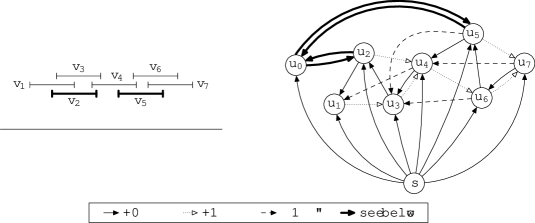
Figure 8: On the left, a unit interval graph with two pre-drawn intervals. On the right, the corresponding digraph $D$ with the weight encoded as in the box. The weights of the bold edges are as follows: $w(u_{0},u_{2})=\hbox{\rm{ubound}}(v_{2})$, $w(u_{0},u_{5})=\hbox{\rm{ubound}}(v_{5})$, $w(u_{2},u_{0})=-\hbox{\rm{lbound}}(v_{2})$, and $w(u_{5},u_{0})=-\hbox{\rm{lbound}}(v_{5})$.

Following [21, Chapter 24.4], if the system is feasible, a solution, which is not necessarily optimal, can be found as follows. We define a weighted digraph $D$ as follows. As the vertices, we have $V(D)=\{s,u_{0},u_{1},\ldots,u_{k}\}$ where $u_{i}$ corresponds to $x_{i}$ and $s$ is a special vertex. For the edges $\vec{E}(D)$, we first have an edge $(s,u_{i})$ of the weight zero for every $u_{i}$. Then for every constraint $x_{i}-x_{j}\leq b_{i,j}$, we add the edge $(u_{j},u_{i})$ of the weight $b_{i,j}$. See Figure 8.

As proved in [21, Chapter 24.4], there are two possible cases. If $G$ contains a negative-weight cycle, then there is no feasible solution for the system. If $G$ does not contain negative-weight cycles, then we define $\delta(s,u_{i})$ as the weight of the minimum-weight path connecting $s$ to $u_{i}$ in $G$. Then we put $x_{i}=\delta(s,u_{i})$ for each $i$ which defines a feasible solution of the system. Moreover, this solution minimizes the objective function $\max\{x_{i}\}-\min\{x_{i}\}$. We next show that this function is equivalent to the objective function in our linear program.

Suppose that we have a solution of our system, satisfying the constraints but not necessarily optimizing the objective function. Because of our assumption that the representation lies in the interval $[1,n+3]$, we know that $\ell_{i}>0$ for all $i$. Therefore, $x_{i}>x_{0}$. So $\min\{x_{i}\}$ is always attained by $x_{0}$, while $\max\{x_{i}\}$ is always attained by $x_{k}$. So minimization of the objective function $\max\{x_{i}\}-\min\{x_{i}\}$ is equivalent to the original minimization of $E_{t}=x_{k}-x_{0}+1$.

In order to find a negative-weight cycle in $D$ or, alternatively, compute the weight of the minimum-weight paths from $s$ to all the other vertices of $D$, we use the Bellman-Ford algorithm. Notice that Dijkstra’s algorithm cannot be used in this case, since some edges of $D$ have negative weight. We next analyze the running time of the whole procedure.

We assume that the cost of arithmetic operations with large numbers is not constant. The algorithm computes the value $\varepsilon$ in the beginning which can be clearly done in time $\mathcal{O}{}(nD(r))$. (Instead of the least common multiple we can simply compute the product of $q_{i}$’s.)

Afterwards, we compute the weights of the edges of $D$ as multiples of $\varepsilon$, which takes time $\mathcal{O}{}(kD(r))$. Then each step of the Bellman-Ford algorithm requires time $\mathcal{O}{}(r)$, and the algorithm runs $\mathcal{O}{}(k^{2})$ steps in total. The total time to solve each linear program is therefore $\mathcal{O}{}(k^{2}r+kD(r))$. Finally, the total time of the algorithm is $\mathcal{O}{}(n^{2}r+nD(r))$.

In the next subsections, we improve the time complexity of the BoundRep problem with prescribed $\blacktriangleleft$ to $\mathcal{O}{}(n^{2}+nD(r))$. Our algorithm makes use of several structural properties of the set of all representations. We note that structural properties of the polyhedron of our linear program, in the case where all lower bounds equal zero and there are no upper bounds, have been considered in several papers in the context of semiorders [29, 30].

5.2 The Partially Ordered Set ${\mathfrak{Rep}}$

Let the graph $G$ in consideration be a connected unit interval graph. We study structural properties of its representations. Suppose that we fix one of the two partial left-to-right orders $<$ of the intervals from Section 3, so that only indistinguishable vertices are incomparable. We also fix some positive $\varepsilon={1\over K}$. For most of this section, we work just with lower bounds and completely ignore upper bounds.

We define ${\mathfrak{Rep}}$ as the set of all $\varepsilon$-grid representations satisfying the lower bounds and in some left-to-right ordering that extends $<$. We define a very natural partial ordering $\leq$ on ${\mathfrak{Rep}}$: We say that ${\cal R}\leq{\cal R}^{\prime}$ if and only if $\ell_{i}\leq\ell^{\prime}_{i}$ for every $v_{i}\in V(G)$; i.e., $\leq$ is the carthesian ordering of vectors $(\ell_{1},\dots,\ell_{n})$. In this section, we study structural properties of the poset $({\mathfrak{Rep}},\leq)$.

If $\varepsilon\leq{1\over n}$, then ${\mathfrak{Rep}}\neq\emptyset$. The reason is that the graph $G$ is a unit interval graph, and thus there always exists an $\varepsilon$-grid representation ${\cal R}$ far to the right satisfying the lower bound contraints.

The Semilattice Structure. Let us assume that $\hbox{\rm{lbound}}(v_{i})>-\infty$ for some $v_{i}\in V(G)$. Let $S$ be a subset of ${\mathfrak{Rep}}$. The infimum $\inf(S)$ is the greatest representation ${\cal R}\in{\mathfrak{Rep}}$ such that ${\cal R}\leq{\cal R}^{\prime}$ for every ${\cal R}^{\prime}\in S$. In a general poset, infimums may not exist, but if they exist, they are always unique. For ${\mathfrak{Rep}}$, we show:

Lemma 5.5

Every non-empty $S\subseteq{\mathfrak{Rep}}$ has an infimum $\inf(S)$.

Proof 10

We construct the requested infimum $\cal R$ as follows:

$$\ell_{i}=\min\{\ell^{\prime}_{i}:{\cal R}^{\prime}\in S\},\qquad\forall v_{i}\in V(G).$$

Notice that the positions in ${\cal R}$ are well-defined, since the position of each interval in each $\cal R^{\prime}$ is bounded and always on the $\varepsilon$-grid. Clearly, if ${\cal R}$ is a correct representation, it is the infimum $\inf(S)$. It remains to show that ${\cal R}\in{\mathfrak{Rep}}$.

Clearly, all positions in ${\cal R}$ belong to the $\varepsilon$-grid and satisfy the lower bound constraints. Let $v_{i}$ and $v_{j}$ be two vertices. The values $\ell_{i}$ and $\ell_{j}$ in ${\cal R}$ are given by two representations ${\cal R}_{1},{\cal R}_{2}\in S$, that is, $\ell_{i}=\ell^{1}_{i}$ and $\ell_{j}=\ell^{2}_{j}$. Notice that the left-to-right order in ${\cal R}$ has to extend $<$: If $v_{i}<v_{j}$, then $\ell_{i}=\ell^{1}_{i}\leq\ell^{2}_{i}<\ell_{j}^{2}=\ell_{j}$, since ${\cal R}_{1}$ minimizes the position of $v_{i}$ and the left-to-right order in ${\cal R}_{2}$ extends $<$. Concerning correctness of the representation of the pair $v_{i}$ and $v_{j}$, we suppose that $\ell_{i}=\ell^{1}_{i}\leq\ell^{2}_{j}=\ell_{j}$; otherwise we swap $v_{i}$ and $v_{j}$.

• First we suppose that $v_{i}v_{j}\in E(G)$. Then $\ell^{2}_{j}\leq\ell^{1}_{j}$, since ${\cal R}_{2}$ minimizes the position of $v_{j}$. Since ${\cal R}_{1}$ is a correct representation, $\ell^{1}_{j}-1\leq\ell^{1}_{i}$. So $\ell_{j}-1\leq\ell_{i}\leq\ell_{j}$, and the intervals $v_{1}$ and $v_{2}$ intersect.

• The other case is when $v_{i}v_{j}\notin E(G)$. Then $\ell^{1}_{i}\leq\ell^{2}_{i}\leq\ell^{2}_{j}-1-\varepsilon$, since ${\cal R}_{1}$ minimizes the position of $v_{i}$, ${\cal R}_{2}$ is a correct representation and $v_{i}<v_{j}$ in both representations. So $v_{i}$ and $v_{j}$ do not intersect in ${\cal R}$ as requested.

Consequently, ${\cal R}$ represents correctly each pair $v_{i}$ and $v_{j}$, and hence ${\cal R}\in{\mathfrak{Rep}}$.

A poset is a (meet)-semilattice if every pair of elements $a,b$ has an infimum $\inf(\{a,b\})$. Lemma 5.5 shows that the poset $({\mathfrak{Rep}},\leq)$ forms a (meet)-semilattice. Similarly as ${\mathfrak{Rep}}$, we could consider the poset set of all ($\varepsilon$-grid) representations satisfying both the lower and the upper bounds. The structure of this poset is a complete lattice, since all subsets have infimums and supremums. Lattices and semilattices are frequently studied, and posets that are lattices satisfy very strong algebraic properties.

The Left-most Representation. We are interested in a specific representation in ${\mathfrak{Rep}}$, called the left-most representation. An $\varepsilon$-grid representation ${\cal R}\in{\mathfrak{Rep}}$ is the left-most representation if ${\cal R}\leq{\cal R}^{\prime}$ for every ${\cal R}^{\prime}\in{\mathfrak{Rep}}$; so the left-most representation is left-most in each interval at the same time. We note that the notion of the left-most representation does not make sense if we consider general representations (not on the $\varepsilon$-grid). The left-most representation is the infimum $\inf({\mathfrak{Rep}})$, and thus by Lemma 5.5 we get:

Corollary 5.6

The left-most representation always exists and it is unique.

There are two algorithmic motivations for studying left-most representations. First, in the linear program of Section 5.1 we need to find a representation minimizing $E_{t}$. Clearly, the left-most representation is minimizing $E_{t}$ and in addition it is minimizing the rest of the endpoints as well. The second motivation is that we want to construct a representation satisfying the upper bounds as well, so it seems reasonable to try to place every interval as far to the left as possible. The left-most representation is indeed a good candidate for a bounded representation:

Lemma 5.7

There exists a representation ${\cal R}^{\prime}$ satisfying both lower and upper bound constraints if and only if the left-most representation ${\cal R}$ satisfies the upper bound constraints.

Proof 11

Since ${\cal R}\in{\mathfrak{Rep}}$, it satisfies the lower bounds. If ${\cal R}$ satisfies the upper bound constraints, it is a bounded representation. On the other hand, let ${\cal R}^{\prime}$ be a bounded representation. Then

$$\hbox{\rm{lbound}}(v_{i})\leq\ell_{i}\leq\ell^{\prime}_{i}\leq\hbox{\rm{ubound}}(v_{i}),\qquad\forall v_{i}\in V(G),$$

and the left-most representation is also a bounded representation.

5.3 Why Left-most Representations Cannot Be Easily Constructed by Iterations?

A very natural idea for an algorithm is to construct the left-most representation iteratively, by adding the vertices $v_{1},\dots,v_{n}$ one by one and recomputing the left-most representation in each step. In this section, we describe why this natural algorithm does not run in quadratic time. More precisely, we do not claim that it is not possible to implement it in quadratic time or faster using some additional tricks and structural results, but we did not succeeded in this matter.

The Iterative Algorithm. Let $G$ be a connected unit interval graph, and let $<$ be the left-to-right partial ordering of its vertices $v_{1},\dots,v_{n}$ numbered from left to right. We denote by $G_{k}$ the graph induced by $\{v_{1},\dots,v_{k}\}$. Let ${\cal R}_{k}$ be the left-most representation of $G_{k}$, and let $\ell_{i}^{k}$ be the position of the left endpoint of $v_{i}$ in ${\cal R}_{k}$. The iterative algorithm runs as follows.

We initiate ${\cal R}_{1}$ with $\ell^{1}_{1}=\hbox{\rm{lbound}}(v_{1})$. To compute ${\cal R}_{k}$ from ${\cal R}_{k-1}$, we first put $\ell^{k}_{i}:=\ell^{k-1}_{i}$ for all $1\leq i\leq k-1$, and $\ell^{k}_{k}:=\max\bigl{\{}\hbox{\rm{lbound}}(v_{k}),\ell^{k}_{j}+1+\varepsilon\bigr{\}}$ where $v_{j}$ is the rightmost placed non-neighbor of $v_{k}$. Since ${\cal R}_{k}$ is not likely a correct representation of $G_{k}$, we proceed by a series of fixes till we obtain a correct representation:

• If $v_{i}v_{j}\in E(G_{k})$, $i<j$, and $\ell^{k}_{i}<\ell^{k}_{j}-1$, we fix ${\cal R}_{k}$ by setting $\ell^{k}_{i}:=\ell^{k}_{j}-1$.

• If $v_{i}v_{j}\notin E(G_{k})$, $i<j$, and $\ell^{k}_{i}\geq\ell^{k}_{j}-1$, we fix ${\cal R}_{k}$ by setting $\ell^{k}_{j}:=\ell^{k}_{i}+1+\varepsilon$.

Correctness. We start by proving that the above algorithm is correct.

Proposition 5.8

The above iterative algorithm stops after finite number of steps and outputs the left-most representation ${\cal R}$.

Proof 12

It is just sufficient to show that it constructs the left-most representation ${\cal R}_{k}$ from the left-most representation ${\cal R}_{k-1}$, and the rest is true by induction. Let ${\cal R}^{s}_{k}$ be a vector of positions created by the algorithm after $s$ fixes, so ${\cal R}^{s}_{k}$ might not be a correct representation. We prove by induction according to $s$ that ${\cal R}^{s}_{k}\leq{\cal R}_{k}$.

Since ${\cal R}_{k-1}$ is the left-most representation of $G_{k-1}$, we get ${\cal R}_{k-1}\leq{\cal R}_{k}|_{G_{k-1}}$. We initiate $\ell^{k}_{k}$ as far to the left as possible, and thus ${\cal R}^{0}_{k}\leq{\cal R}_{k}$. Now let ${\cal R}^{s-1}_{k}\leq{\cal R}_{k}$. Then we easily get ${\cal R}^{s}_{k}\leq{\cal R}_{k}$ since the fix of $(v_{i},v_{j})$ shifts one of them as little to the right as necessary; since ${\cal R}_{k}$ is a correct representation, it clearly cannot have the shifted interval more to the left than ${\cal R}^{s}_{k}$.

Since each fix strictly increases the position of one interval and according to Corrolary 5.6 the left-most representation ${\cal R}_{k}$ always exists, we cannot apply fixes indefinitely and the algorithm outputs some correct representation ${\cal R}^{s}_{k}$. Since ${\cal R}^{s}_{k}\leq{\cal R}_{k}$, we get ${\cal R}^{s}_{k}={\cal R}_{k}$.

Unclear Complexity. Even though the above algorithm is correct, it is not even clear that its complexity is polynomial in $n$ and does not depend on $\varepsilon$. We did not try to further estimate this complexity but it seems one could bound the number of fixes in each iteration by something like $\mathcal{O}{}(n^{2})$ which would give a cubic-time algorithm. The reason why this does not give a quadratic-time algorithm is that the position of each interval can be updated by multiple fixes. We always shift as little as possible, and not as much as it is required by the structure of the graph. Furthermore, we simplified our analysis by assuming that we can locate a wrongly represented pair $(v_{i},v_{j})$ in constant time, and that we compute on the arithmetic machine (so we ignored numerical issues with small values of $\varepsilon$).

Nevertheless, we believe that the complexity of this algorithm could be improved which might lead to a different quadratic-time (or potentially even linear-time) algorithm for the bounded representation problem with prescribed ordering $\vartriangleleft$. As a good starting point, we suggest that one should get a good structural understand how much ${\cal R}_{k}$ differs from ${\cal R}_{k-1}$. Even through we give some additional properties concerning the left-most representation, we still do not fully understand its structure. Therefore we derived a different algorithm based on shifting which we describe in the rest of Section 5.

5.4 Left-Shifting of Intervals

Suppose that we construct some initial $\varepsilon$-grid representation that is not the left-most representation. We want to transform this initial representation in ${\mathfrak{Rep}}$ into the left-most representation of ${\mathfrak{Rep}}$ by applying a sequence of the following simple operations called the left-shifting. The left-shifting operation shifts one interval of the representations by $\varepsilon$ to the left such that this shift maintains the correctness of the representation; for an example see Figure 9a. The main goal of this section is to prove that by left-shifting we can always produce the left-most representation.

Figure 9: (a) A representation modified by left-shifting of $v_{6}$ and $v_{4}$. (b) The corresponding obstruction digraphs $H$ for each of the representations. Only sinks of the obstruction digraphs can be left-shifted.

Proposition 5.9

For $\varepsilon={1\over K}$ and $K\geq{n\over 2}$, an $\varepsilon$-grid representation ${\cal R}\in{\mathfrak{Rep}}$ is the left-most representation if and only if it is not possible to shift any single interval to the left by $\varepsilon$ while maintaining correctness of the representation.

Before proving the proposition, we describe some additional combinatorial structure of left-shifting. An interval $v_{i}$ is called fixed if it is in the left-most position and cannot ever be shifted more to the left, i.e., $\ell_{i}=\min\{\ell^{\prime}_{i}:{\cal R}^{\prime}\in{\mathfrak{Rep}}\}$. For example, an interval $v_{i}$ is fixed if $\ell_{i}=\hbox{\rm{lbound}}(v_{i})$. A representation is the left-most representation if and only if every interval is fixed.

Obstruction Digraph. An interval $v_{i}$, having $\ell_{i}>\hbox{\rm{lbound}}(v_{i})$, can be left-shifted if it does not make the representation incorrect, and the incorrectness can be obtained in two ways. First, there could be some interval $v_{j}$, $v_{j}\vartriangleleft v_{i}$ such that $v_{i}v_{j}\notin E(G)$ and $\ell_{j}+1+\varepsilon=\ell_{i}$; we call $v_{j}$ a left obstruction of $v_{i}$. Second, there could be some interval $v_{j}$, $v_{i}\vartriangleleft v_{j}$ such that $v_{i}v_{j}\in E(G)$ and $\ell_{i}+1=\ell_{j}$ (so $v_{i}$ and $v_{j}$ are touching); then we call $v_{j}$ a right obstruction of $v_{i}$. In both cases, we first need to move $v_{j}$ before moving $v_{i}$.

For the current representation ${\cal R}$, we define the obstruction digraph $H$ on the vertices of $G$ as follows. We put $V(H)=V(G)$ and $(v_{i},v_{j})\in E(H)$ if and only if $v_{j}$ is an obstruction of $v_{i}$. For an edge $(v_{i},v_{j})$, if $v_{j}\vartriangleleft v_{i}$, we call it a left edge; if $v_{i}\vartriangleleft v_{j}$, we call it a right edge. As we apply left-shifting, the structure of $H$ changes; see Figure 9b.

Lemma 5.10

An interval $v_{i}$ is fixed if and only if there exists a directed path in $H$ from $v_{i}$ to $v_{j}$ such that $\ell_{j}=\hbox{\rm{lbound}}(v_{j})$.

Proof 13

Suppose that $v_{i}$ is connected to $v_{j}$ by a path in $H$. By the definition of $H$, $v_{x}v_{y}\in E(H)$ implies that $v_{y}$ has to be shifted before $v_{x}$. Thus $v_{j}$ has to be shifted before moving $v_{i}$ which is not possible since $\ell_{j}=\hbox{\rm{lbound}}(v_{j})$.

On the other hand, suppose that $v_{i}$ is fixed, i.e., $\ell_{i}=\inf\{\ell^{\prime}_{i}:\forall{\cal R^{\prime}}\}$. Let $H^{\prime}$ be the induced subgraph of $H$ of the vertices $v_{j}$ such that there exists a directed path from $v_{i}$ to $v_{j}$. If for all $v_{j}\in H^{\prime}$, $\ell_{j}>\hbox{\rm{lbound}}(v_{j})$, we can shift all vertices of $H^{\prime}$ by $\varepsilon$ to the left which constructs a correct representation and contradicts that $v_{i}$ is fixed. Therefore, there exists $v_{j}\in H^{\prime}$ having $\ell_{j}=\hbox{\rm{lbound}}(v_{j})$ as requested.

For example in Figure 9 on the left, if $\ell_{4}=\hbox{\rm{lbound}}(v_{4})$, then the intervals $v_{3}$, $v_{4}$, $v_{5}$ and $v_{7}$ are fixed. Also, we can prove:

Lemma 5.11

If $\varepsilon={1\over K}$ and $K\geq{n\over 2}$, the obstruction digraph $H$ is acyclic.

Proof 14

Suppose for contradiction that $H$ contains some cycle $u_{1},\dots,u_{c}$. This cycle contains $a$ left edges and $b$ right edges. Recall that if $(u_{i},u_{i+1})$ is a left edge, then $\ell_{u_{i+1}}=\ell_{u_{i}}-1-\varepsilon$, and if it is a right edge, $\ell_{u_{i+1}}=\ell_{u_{i}}+1$ (and similarly for $(u_{c},u_{1})$). If we go along the cycle from $u_{1}$ to $u_{1}$, the initial and the final positions have to be the same. Therefore $a(1+\varepsilon)=b$.

Now if this equation holds, then $a$ has to be a multiple of $K$. Therefore $a\geq K$ and $b\geq K+1$, and thus $n\geq c=a+b\geq 2K+1$ which is not possible.

We note that the assumption $K\geq{n\over 2}$ is necessary and tight. For every $\varepsilon={1\over K}$, there exists a representation of a graph with $2K+1$ vertices having a cycle in $H$. The graph contains two cliques $v_{0},\dots,v_{K-1}$ and $w_{0},\dots,w_{K}$ such that $v_{i}$ is also adjacent to $w_{0},\dots,w_{i}$. Then the assignment $\ell_{v_{0}}=0$, $\ell_{v_{i}}=\ell_{v_{0}}+i\varepsilon$ and $\ell_{w_{i}}=\ell_{v_{0}}+1+i\varepsilon$ is a correct representation. Observe that $H$ contains a cycle $w_{k}v_{k-1}w_{k-1}v_{k-2}w_{k-2}\dots v_{1}w_{1}v_{0}w_{0}w_{k}$. See Figure 10 for $K=3$.

Figure 10: An $\varepsilon$-grid representation for $\varepsilon={1\over 3}$ on the left and the obstruction digraph $H$ containing a cycle on the right.

Predecessors of Poset ${\mathfrak{Rep}}$. A representation ${\cal R}^{\prime}\in{\mathfrak{Rep}}$ is a predecessor of ${\cal R}\in{\mathfrak{Rep}}$ if ${\cal R}^{\prime}<{\cal R}$ and there is no representation $\bar{\cal R}\in{\mathfrak{Rep}}$ such that ${\cal R}^{\prime}<\bar{\cal R}<{\cal R}$. We denote the predecessor relation by $\prec$. In a general poset, predecessors may not exist. But they always exist for a poset of a discrete structure like $({\mathfrak{Rep}},\leq)$: Indeed, there are finitely many representations $\bar{\cal R}$ between any ${\cal R}^{\prime}<{\cal R}$, and thus the predecessors always exist. Also, for any two representations ${\cal R}^{\prime}<{\cal R}$, there exists a finite chain of predecessors ${\cal R}^{\prime}={\cal R}_{0}\prec{\cal R}_{1}\prec\cdots\prec{\cal R}_{k}={\cal R}$.

For the poset $({\mathfrak{Rep}},\leq)$, we are able to fully describe the predecessor structure:

Lemma 5.12

For $\varepsilon={1\over K}$ and $K\geq{n\over 2}$, the representation ${\cal R}^{\prime}$ is a predecessor of ${\cal R}$ if and only if ${\cal R}^{\prime}$ is obtained from ${\cal R}$ by applying one left-shifting operation.

Proof 15

Clearly, if ${\cal R}^{\prime}$ is obtained from ${\cal R}$ by one left-shifting, it is a predecessor of ${\cal R}$.

On the other hand, suppose we have ${\cal R}^{\prime}<{\cal R}$. Let $H$ be the obstruction digraph of ${\cal R}$ and $\bar{H}$ be the subgraph of $H$ induced by the intervals having different positions in ${\cal R}$ and ${\cal R}^{\prime}$. Then there are no directed edges from $\bar{H}$ to $H\setminus\bar{H}$ (otherwise ${\cal R}^{\prime}$ would be an incorrect representation). According to Lemma 5.11, the digraph $\bar{H}$ is acyclic. Therefore, it contains at least one sink $v_{i}$. By left-shifting $v_{i}$ in ${\cal R}$, we create a correct representation $\bar{\cal R}\in{\mathfrak{Rep}}$. Clearly, ${\cal R}^{\prime}\leq\bar{\cal R}\prec{\cal R}$, and so ${\cal R}^{\prime}$ is a predecessor of ${\cal R}$ if and only if ${\cal R}^{\prime}=\bar{\cal R}$.

Again, the assumption on the value of $\varepsilon$ is necessary. For example in Figure 10, the structure of ${\mathfrak{Rep}}$ is just a single chain where a predecessor of some representation is obtained by shifting all intervals by $\varepsilon$ to the left.

Proof of Left-shifting Proposition. The main proposition of this subsection is a simple corollary of Lemma 5.12.

Proof 16 (Proposition 5.9)

The left-most representation ${\cal R}$ is $\inf({\mathfrak{Rep}})$, so it has no predecessors and nothing can be left-shifted. On the other hand, if $\inf({\mathfrak{Rep}})<{\cal R}$, there is a chain of predecessors in between which implies using Lemma 5.12 that it is possible to left-shift some interval.

5.5 Preliminaries for the Shifting Algorithm

Before describing the shifting algorithm, we present several results which simplify the graph and the description of the algorithm.

Pruned Graph. The obstruction digraph $H$ may contain many edges since each vertex $v_{i}$ can have many obstructions. But if $v_{i}$ has many, say, left obstructions, these obstructions have to be positioned the same. If two intervals $u$ and $v$ have the same position in a correct unit interval representation, then $N[u]=N[v]$ and they are indistinguishable. Our goal is to construct a pruned graph $G^{\prime}$ which replaces each group of indistinguishable vertices of $G$ by a single vertex. This construction is not completely straightforward since indistinguishable vertices may have different lower and upper bounds.

Let $\{\Gamma_{1},\dots,\Gamma_{k}\}$ be the partitioning of $V(G)$ by the groups of indistinguishable vertices (and the groups are ordered by $\vartriangleleft$ from left to right). We construct a unit interval graph $G^{\prime}$, where the vertices are $\gamma_{1},\dots,\gamma_{k}$ with $\hbox{\rm{lbound}}(\gamma_{i})=\max\{\hbox{\rm{lbound}}(v_{j}):v_{j}\in\Gamma_{i}\}$, and the edges $E(G^{\prime})$ correspond to the edges between the groups of $G$.

Suppose that we have the left-most representation ${\cal R}^{\prime}$ of the pruned graph $G^{\prime}$ and we want to construct the left-most representation ${\cal R}$ of $G$. Let $\Gamma_{\ell}$ be a group. We place each interval $v_{i}\in\Gamma_{\ell}$ as follows. Let $\gamma^{\ell}_{\leftarrow}$ be the first non-neighbor of $\gamma_{\ell}$ on the left and $\gamma^{\ell}_{\rightarrow}$ be the right-most neighbor of $\gamma_{\ell}$ (possibly $\gamma^{\ell}_{\rightarrow}=\gamma_{\ell}$). We set

$$\ell_{i}=\max\{\hbox{\rm{lbound}}(v_{i}),\ell_{\gamma^{\ell}_{\leftarrow}}+1+\varepsilon,\ell_{\gamma^{\ell}_{\rightarrow}}-1\},$$ (7)

and if $\gamma^{\ell}_{\leftarrow}$ does not exist, we ignore it in $\max$. The meaning of this formula is to place each interval as far to the left as possible while maintaining the structure of ${\cal R}^{\prime}$. Figure 11 contains an example of the construction of ${\cal R}$.

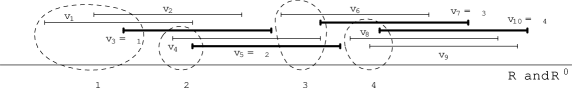
Figure 11: Both representations ${\cal R}$ and ${\cal R}^{\prime}$ in one figure, with the intervals of ${\cal R}^{\prime}$ depicted in bold. The left endpoints of the intervals of each group are enclosed by dashed curves, and these curves are ordered from left to right according to $<$.

Before proving correctness of the construction of ${\cal R}$, we show two general properties of the formula (7). The first lemma states that each interval $v_{i}\in\Gamma_{\ell}$ is not placed in ${\cal R}$ too far from the position of $\gamma_{\ell}$ is ${\cal R}^{\prime}$.

Lemma 5.13

For each $v_{i}\in\Gamma_{\ell}$, it holds

$$\ell_{\gamma_{\ell}}-1\leq\ell_{i}\leq\ell_{\gamma_{\ell}}.$$ (8)

Proof 17

The first inequality is true since $\ell_{\gamma_{\ell}}-1\leq\ell_{\gamma^{\ell}_{\rightarrow}}-1\leq\ell_{i}$ holds according to (7) and the ordering $\vartriangleleft$ for ${\cal R}^{\prime}$. The second inequality holds since ${\cal R}^{\prime}$ is a correct bounded representation, and so $\ell_{\gamma_{\ell}}$ is greater than or equal to each term in (7).

The second lemma states that the representations ${\cal R}$ and ${\cal R}^{\prime}$ are intertwining each other. If ${\cal R}$ is drawn on top of ${\cal R}^{\prime}$, then the vertices of each group $\Gamma_{\ell}$ are in between of $\gamma_{\ell-1}$ and $\gamma_{\ell}$; see Figure 11.

Lemma 5.14

For each $v_{i}\in\Gamma_{\ell}$ and $\ell>1$, it holds

$$\ell_{\gamma_{\ell-1}}<\ell_{i}\leq\ell_{\gamma_{\ell}},$$ (9)

Proof 18

The second inequality holds by (8). For the first inequality, there are two possible cases why the groups $\Gamma_{\ell-1}$ and $\Gamma_{\ell}$ are distinct:

• The first case is when $\gamma^{\ell}_{\leftarrow}$ is a neighbor of $\gamma_{\ell-1}$. Then $\ell_{\gamma_{\ell-1}}\leq\ell_{\gamma_{\leftarrow}^{\ell}}+1<\ell_{i}$; the first inequality holds since $\gamma_{\leftarrow}^{\ell}\gamma_{\ell-1}\in E(G^{\prime})$ and ${\cal R}^{\prime}$ is a correct representation, and the second inequality is given by (7).

• The second case is when $\gamma^{\ell}_{\rightarrow}$ is a non-neighbor of $\gamma_{\ell-1}$. Then $\ell_{\gamma_{\ell-1}}<\ell_{\gamma_{\rightarrow}^{\ell}}-1\leq\ell_{i}$ by the fact that $\gamma_{\ell-1}\gamma_{\rightarrow}^{\ell}\notin E(G^{\prime})$ and by (7).

In both cases, we get $\ell_{\gamma_{\ell-1}}<\ell_{i}$.

Now, we are ready to show correctness of the construction of ${\cal R}$.

Proposition 5.15

From the left-most representation ${\cal R}^{\prime}$ of the pruned graph $G^{\prime}$, we can construct the correct left-most representation ${\cal R}$ of $G$ by placing the intervals according to (7).

Proof 19

We argue the correctness of the representation ${\cal R}$. Let $v_{i}$ and $v_{j}$ be a pair of vertices of $G$. Let $v_{i}v_{j}\in E(G)$. If $v_{i}$ and $v_{j}$ belong to the same group $\Gamma_{\ell}$, they intersect each other at position $\ell_{\gamma_{\ell}}$ by (8). Otherwise let $v_{i}\in\Gamma_{\ell}$ and $v_{j}\in\Gamma_{\ell^{\prime}}$, and assume that $\Gamma_{\ell}<\Gamma_{\ell^{\prime}}$. Then $\ell_{i}\leq\ell_{\gamma_{\ell}}\leq\ell_{j}$ by the intertwining property (9). Also, $\ell_{j}\leq\ell_{\gamma_{\ell^{\prime}}}\leq\ell_{\gamma^{\ell}_{\rightarrow}}\leq\ell_{i}+1$ since $\gamma_{\ell^{\prime}}$ is a right neighbor of $\gamma_{\ell}$ and (8). Therefore, $\ell_{i}\leq\ell_{j}\leq\ell_{i}+1$ and $v_{i}$ intersects $v_{j}$ in ${\cal R}$. Now, let $v_{i}v_{j}\notin E(G)$, $v_{i}\in\Gamma_{\ell}$, $v_{j}\in\Gamma_{\ell^{\prime}}$ and $v_{i}<v_{j}$. Then $\ell_{i}\leq\ell_{\gamma_{\ell}}\leq\ell_{\gamma^{\ell^{\prime}}_{\leftarrow}}\leq\ell_{j}-1-\varepsilon$ by (7) and (8), so $v_{i}$ and $v_{j}$ do not intersect. So the assignment ${\cal R}$ is a correct representation of $G$.

It remains to show that ${\cal R}$ is the left-most representation of $G$. We can identify each $\gamma_{\ell}$ with one interval $v_{i}\in\Gamma_{\ell}$ having $\hbox{\rm{lbound}}(v_{i})=\hbox{\rm{lbound}}(\gamma_{\ell})$; for an example see Figure 11. So $G^{\prime}$ can be viewed as an induced subgraph of $G$. We want to show that the intervals of $G^{\prime}$ are represented in ${\cal R}$ exactly the same as in ${\cal R}^{\prime}$. Since ${\cal R}|_{G^{\prime}}$ (which denotes ${\cal R}$ restricted to $G^{\prime}$) is some representation of $G^{\prime}$ and ${\cal R}^{\prime}$ is the left-most representation of $G^{\prime}$, we get $\ell^{\prime}_{\gamma_{\ell}}\leq\ell_{\gamma_{\ell}}$ for every $\gamma_{\ell}$. By (8), we get $\ell^{\prime}_{\gamma_{\ell}}=\ell_{\gamma_{\ell}}$.

We know that ${\cal R}|_{G^{\prime}}$ is the left-most representation, or in other words each interval of $G^{\prime}$ is fixed in ${\cal R}$. The rest of the intervals are placed so that they are either trivially fixed by $\ell_{i}=\hbox{\rm{lbound}}(v_{i})$, or they have as obstructions some fixed intervals from $G^{\prime}$, in which case they are fixed by Lemma 5.10. Therefore, every interval of $G$ is fixed and ${\cal R}$ is the left-most representation.

For the pruned graph $G^{\prime}$, the obstruction digraph $H$ has in- and out-degree at most two. Each interval has at most one left obstruction and at most one right obstruction, and these obstructions are always the same intervals. More precisely, if $v_{j}$ is a left obstruction of $v_{i}$, then $v_{j}=v_{\leftarrow}^{i}$, whereas if $v_{j}$ is a right obstruction of $v_{i}$, then $v_{j}=v_{\rightarrow}^{i}$.

The pruning operation can be done in time $\mathcal{O}{}(n+m)$, so we may assume that our graph $G$ is already pruned and contains no indistinguishable vertices. And the structure of obstructions in $G$ can be computed in time $\mathcal{O}{}(n+m)$ as well.

Position Cycle. For each interval in some $\varepsilon$-grid representation, we can write its position in this form:

$$\ell_{i}=\alpha_{i}+\beta_{i}\varepsilon,\qquad\alpha_{i}\in{\mathbb{Z}},\ \beta_{i}\in{\mathbb{Z}}_{K},$$ (10)

where $\varepsilon={1\over K}$. In other words, $\alpha_{i}$ is the integer position of $v_{i}$ in the grid and $\beta_{i}$ describes how far is this interval from this integer position.

Concerning left-shifting, the values $\beta_{i}$ are more important. We can depict ${\mathbb{Z}}_{K}=\{0,\dots,K-1\}$ as a cycle with $K$ vertices where the value decreases clockwise. The value $\beta_{i}$ assigns to each interval $v_{i}$ one vertex of the cycle. The cycle ${\mathbb{Z}}_{K}$ together with marked positions of $\beta_{i}$’s is called the position cycle. A vertex of the position cycle is called taken if some $\beta_{i}$ is assigned to it, and empty otherwise. The position cycle allows us to visualize and work with left-shifting very intuitively. When an interval $v_{i}$ is left-shifted, $\beta_{i}$ cyclically decreases by one, so $\beta_{i}$ moves clockwise along the cycle. For an illustration, see Figure 12.

Figure 12: Examples of position cycles. In the cycle on the left, we can shift $\beta_{2}$ in the clockwise direction towards $\beta_{6}$, which gives a new representation whose position cycle is depicted on the right. We note that after this left-shifting, $v_{6}$ is not necessarily an obstruction of $v_{2}$.

If $(v_{i},v_{j})$ is a left edge of $H$, then $\beta_{j}=\beta_{i}-1$, and if $(v_{i},v_{j})$ is a right edge, then $\beta_{i}=\beta_{j}$. So if $v_{j}$ is an obstruction of $v_{i}$, $\beta_{j}$ has to be very close to $\beta_{i}$ (either at the same position or at the next clockwise position). If there is a big empty space in the clockwise direction from $\beta_{i}$, the interval $v_{i}$ can be left-shifted many times (or till it becomes fixed by $\ell_{i}=\hbox{\rm{lbound}}(v_{i})$). Notice that if $\beta_{i}$ is very close to $\beta_{j}$, it does not mean that $\ell_{i}$ is very close to $\ell_{j}$ because the values $\alpha_{i}$ and $\alpha_{j}$ are ignored in the position cycle.

5.6 The Shifting Algorithm for BoundRep

We want to solve an instance of BoundRep with a prescribed ordering $\blacktriangleleft$. We work with an $\varepsilon$-grid which is different from the one in Section 4.1. The new value of $\varepsilon$ is the value given by (1) refined $n$ times, so

$$\varepsilon={1\over n^{2}}\cdot\varepsilon^{\prime}.$$

Lemma 4.1 applies for this value of $\varepsilon$ as well, so if the instance is solvable, there exists a solution which is on this $\varepsilon$-grid.

The algorithm works exactly as the algorithm of Subsection 5.1. The only difference is that for a component with $k$ vertices we can solve the linear program in time $\mathcal{O}{}(k^{2}+kD(r))$, and now we describe how to do it. We assume that the input component is already pruned, otherwise we prune it and use Proposition 5.15 to complete the representation. We expect that the left-to-right order $\vartriangleleft$ of the vertices is given. The algorithm requires time $\mathcal{O}{}(kD(r))$ since the bounds are given in the form $p_{i}\over q_{i}$ and we need to perform arithmetic operations with these bounds. Therefore the total complexity of the algorithm for the BoundRep problem is $\mathcal{O}{}(n^{2}+nD(r))$.

Overview. The algorithm for solving one linear program works in three basic steps:

1. We construct an initial $\varepsilon$-grid representation (in the ordering $\vartriangleleft$) having $\ell_{i}\geq\hbox{\rm{lbound}}(v_{i})$ for all intervals, using the algorithm of Corneil et al. [26].

2. We shift the intervals to the left while maintaining correctness of the representation until the left-most representation is constructed, using Proposition 5.9.

3. We check whether the left-most representation satisfies the upper bounds. If so, we have the left-most representation satisfying all bound constraints. This representation solves the linear program of Subsection 5.1 and minimizes $E_{t}$. Otherwise, the left-most representation does not satisfy the upper bound constraints. Thus by Lemma 5.7 no representation satisfies the upper bound constraints, and the linear program has no solution.

Input Size. Let $r$ be the size of the input describing bound constraints. A standard complexity assumption is that we can operate with polynomially large numbers (having $\mathcal{O}{}(\log r)$ bits in binary) in constant time, to avoid the extra factor $\mathcal{O}{}(\log r)$ in the complexity of most of the algorithms. However, the value of $\varepsilon$ given by (1) might require $\mathcal{O}{}(r)$ digits when written in binary. The assumption that we can computate with numbers having $\mathcal{O}{}(r)$ digits in contant time would break most of the computational models. Therefore, our computational model requires a larger time for arithmetic operations with numbers having $\mathcal{O}{}(r)$ digits in binary. For example, the best known algorithm for multiplication/division on a Turing machine requires time $\mathcal{O}{}(D(r))$.

The problem is that a straightforward implementation of our algorithm working with the $\varepsilon$-grid would require time $\mathcal{O}{}(k^{2}r^{c})$ for some $c$ instead of $\mathcal{O}{}(k^{2}+kD(r))$. There is an easy way out. Instead of computing with long numbers having $\mathcal{O}{}(r)$ digits, we mostly compute with short numbers having just $\mathcal{O}{}(\log r)$ digits. Instead of the $\varepsilon$-grid, we mostly work in a larger $\Delta$-grid where $\Delta={1\over n^{2}}$. The algorithm computes with the long numbers only in two places. First, some initial computations concerning the input are performed. Second, when the shifting makes some interval fixed, the algorithm estimes the final $\varepsilon$-grid position of the interval. All these computations can be done in total time $\mathcal{O}{}(kD(r))$ and we describe everything in detail later.

Left-Shifting. The basic operation of the algorithm is the LeftShift procedure which we describe here. We deal separately with fixed and unfixed intervals (and some intervals might be fixed initially). Unfixed intervals are on the $\Delta$-grid and fixed intervals have precise positions calculated on the $\varepsilon$-grid. We place only unfixed intervals on the position cycle for the $\Delta$-grid. At any moment of the algorithm, each vertex of the position cycle is taken by at most one $\beta_{i}$; this is true for the initial representation and the shifting keeps this property.

We define the procedure $\hbox{\rm\sc LeftShift}(v_{i})$ which shifts $v_{i}$ from the position $\ell_{i}$ into a new position $\ell^{\prime}_{i}$ such that the representation remains correct. The procedure $\hbox{\rm\sc LeftShift}(v_{i})$ consists of two steps:

1. Since $v_{i}$ is unfixed, it has some $\beta_{i}$ placed on the position cycle. Let $k$ be such that the vertices $\beta_{i}+1,\dots,\beta_{i}+k$ of the position cycle are empty and the vertex $\beta_{i}+k+1$ is taken by some $\beta_{b}$. Then a candidate for the new position of $v_{i}$ is $\bar{\ell}_{i}=\ell_{i}-k\Delta$.

2. We need to ensure that this shift from $\ell_{i}$ to $\bar{\ell}_{i}$ is valid with respect to $\hbox{\rm{lbound}}(v_{i})$ and the positions of the fixed intervals. Concerning the lower bound, we cannot shift further than $\hbox{\rm{lbound}}(v_{i})$. Concerning the fixed intervals, the shift is limited by positions of fixed obstructions of $v_{i}$. If $v_{j}$ is a fixed left obstruction, we cannot shift further than $\ell_{j}+1+\varepsilon$, and if $v_{j^{\prime}}$ a fixed right obstruction, we cannot shift further than $\ell_{j^{\prime}}-1$.

The resulting position after applying $\hbox{\rm\sc LeftShift}(v_{i})$ is

$$\ell^{\prime}_{i}=\max\{\bar{\ell}_{i},\hbox{\rm{lbound}}(v_{i}),\ell_{j}+1+\varepsilon,\ell_{j^{\prime}}-1\}.$$ (11)

Lemma 5.16

If the original representation ${\cal R}$ is correct, than the $\hbox{\rm\sc LeftShift}(v_{i})$ procedure produces a correct representation ${\cal R}^{\prime}$.

Proof 20

Clearly, the lower bound for $v_{i}$ is satisfied in ${\cal R}^{\prime}$. The shift of $v_{i}$ from $\ell_{i}$ to $\ell^{\prime}_{i}$ can be viewed as a repeated application of the left-shifting operation from Section 5.4. We just need to argue that each left-shifting operation can be applied till the position $\ell^{\prime}_{i}$ is reached.

If at some point, the left-shifting operation could not be applied, there would have to be some obstruction $v_{j}$ of $v_{i}$. There is no unfixed obstruction since all vertices of the position cycle $\beta_{i}+1,\dots,\beta_{i}+k$ are empty. And $v_{j}$ cannot be fixed as well since we check positions of both possible obstructions. So there is no obstruction $v_{j}$. Therefore, by repeated applying the left-shifting operation, the interval $v_{i}$ gets at a position $\ell^{\prime}_{i}$ and the resulting representation is correct.

After $\hbox{\rm\sc LeftShift}(v_{i})$, if $\bar{\ell}_{i}$ is not a strict maximum of the four terms in (11), the interval $v_{i}$ becomes fixed; either trivially since $\ell^{\prime}_{i}=\hbox{\rm{lbound}}(v_{i})$, or by Lemma 5.10 since $v_{i}$ becomes obstructed by some fixed interval. In such a case, we remove $\beta_{i}$ from the position cycle.

Fast Implementation of Left-Shifting. Since we apply the LeftShift procedure repeatedly, we want to implement it in time $\mathcal{O}{}(1)$. Considering the terms in (11), the first term $\bar{\ell}_{i}$ is a short number (on the $\Delta$-grid) and the remaining terms are long numbers (on the $\varepsilon$-grid). We first compare $\bar{\ell}_{i}$ to the remaining terms which are three comparisons of short and long numbers and we are going to show how to compare them in $\mathcal{O}{}(1)$. If $\bar{\ell}_{i}$ is a strict maximum, we use it for $\ell^{\prime}_{i}$. Otherwise, we need to compute the maximum of the remaining three terms which takes time $\mathcal{O}{}(D(r))$. But then the interval $v_{i}$ becomes fixed, and so this costly step is done exactly $k$ times, and takes the total time $\mathcal{O}{}(kD(r))$.

Lemma 5.17

With the total precomputation time $\mathcal{O}{}(kD(r))$, it is possible to compare $\bar{\ell}_{i}$ to the remaining terms in (11) in time $\mathcal{O}{}(1)$ per LeftShift procedure.

Proof 21

Initially, we do the following precomputation for the lower bounds. By the input, we have $b$ lower bounds given in the form ${p_{1}\over q_{1}},\dots,{p_{b}\over q_{b}}$ as irreducible fractions. For each bound, we first compute its position $(\alpha_{i},\beta_{i})$ on the $\varepsilon$-grid; see (10).

If $\hbox{\rm{lbound}}(v_{i})\ll\hbox{\rm{lbound}}(v_{j})$ for some vertices $v_{i}$ and $v_{j}$, then $\hbox{\rm{lbound}}(v_{i})$ is never achieved since the graph is connected and every representation takes space at most $k$. Therefore we can increase $\hbox{\rm{lbound}}(v_{i})$ without any change in the solution of the instance. More precisely, let $\alpha=\max\alpha_{i}$. Then we modify each bound by setting $\alpha_{i}:=\max\{\alpha-k-1,\alpha_{i}\}$. In addition, we shift all the bounds by substructing a constant $C$ such that each $\alpha_{i}-C\in[0,k+1]$. Concerning $\beta_{i}$, we round the position $(\alpha_{i},\beta_{i})$ down to a position $(\alpha_{i},\bar{\beta}_{i})$ of the $\Delta$-grid. These precomputations can be done for all lower bounds in time $\mathcal{O}{}(kD(r))$.

Suppose that we want to find out whether $\bar{\ell}_{i}\leq\hbox{\rm{lbound}}(v_{j})=\alpha_{j}+\beta_{j}\cdot\varepsilon$ where $\bar{\ell}_{i}$ is in the $\Delta$-grid. Then it is sufficient to check whether $\bar{\ell}_{i}\leq\alpha_{j}+\bar{\beta}_{j}\Delta$ which can be done in constant time since both $\alpha_{j}$ and $\bar{\beta}_{j}$ are short numbers.

When $v_{j}$ becomes fixed, its precise position is computed using (11). Then we compute the values $\ell_{j}-1$ and $\ell_{j}+1+\varepsilon$ used in (11) and round them down to the $\Delta$-grid. Using these precomputed values, $\bar{\ell}_{i}$ can be compared with the remaining terms in (11) in time $\mathcal{O}{}(1)$. When an interval becomes fixed, time $\mathcal{O}{}(D(r))$ is used. Since each interval becomes fixed exactly once, this rounding also takes the total time $\mathcal{O}{}(kD(r))$.

Notice that the representation is constructed in a position shifted by $C$. Later, before checking the upper bound, we shift the whole representation back.

Initial Representation. Recall that the position cycle has $n^{2}$ vertices and $\Delta={1\over n^{2}}$. The algorithm of Corneil et al. [26] gives a representation in the $1\over k$-grid. Using the proof of Lemma 4.1, we construct from it the initial $\Delta$-grid representation. Then we shift it such that $\ell_{i}\geq\hbox{\rm{lbound}}(v_{i})$ for each $v_{i}$ and $\ell_{i}\leq\hbox{\rm{lbound}}(v_{i})+\Delta$ for some $v_{i}$. For this initial representation, each interval can be shifted to the left in total by at most $\mathcal{O}{}(k)$.

The initial representation obtained from the representation of the algorithm of Corneil et al. [26] places all intervals in such a way that $\beta_{i}$’s are almost positioned equidistantly in the position cycle; refer to the left-most position cycle in Figure 13. As we say in the description of the LeftShift procedure, we only require that all $\beta_{i}$’s are placed to pairwise different vertices of the position cycle.

Figure 13: The position cycle during the first phase, changing from left to right. The first phase clusters the $\beta_{i}$’s by moving $\beta_{4}$, $\beta_{5}$, $\beta_{2}$ and $\beta_{3}$ towards $\beta_{1}$. When $\hbox{\rm\sc LeftShift}(v_{2})$ is applied, $v_{2}$ becomes fixed and $\beta_{2}$ disappears from the position cycle.

Shifting Phases. All shifting of the algorithm is done by repeated application of the LeftShift procedure. Using Lemma 5.16, we know that the representation created in each step is correct. We apply the procedure in such a way that each interval is almost always shifted by almost one. The shifting of unfixed intervals proceeds in two phases:

• The first phase creates one big gap by clustering all $\beta_{i}$’s in one part of the cycle. To do so, we apply the LeftShift procedure to each interval, in the order given by the position cycle. Of course, some intervals might become fixed and disappear from the position cycle. We obtain one big gap of size at least $n(n-1)$. Again, refer to Figure 13.

• In the second phase, we use this big gap to shift intervals one by one, which also moves the cluster along the position cycle. Again, if some interval becomes fixed, it is removed from the position cycle. The second phase finishes when each interval becomes fixed and the left-most representation is constructed. For an example, see Figure 14.

Figure 14: The position cycle during the second phase, changing from left to right. We shift $\beta_{i}$’s across the big gap till all $\beta_{i}$’s disappear.

Putting It All Together. First, we show correctness of the shifting algorithm and its complexity:

Lemma 5.18

For a component having $k$ vertices, the shifting algorithm constructs a correct left-most representation in time $\mathcal{O}{}(k^{2}+kD(r))$.

Proof 22

First, we argue correctness of the algorithm. The algorithm starts with an initial representation which is correct and satisfies the lower bounds. By Lemma 5.16, after applying each LeftShift procedure, the resulting representation is still correct. The algorithm keeps a correct list of fixed intervals which is increased by shifting. So after finitely many applications of the LeftShift procedure, every interval becomes fixed, and we obtain the left-most representation.

Concerning complexity, all precomputations take total time $\mathcal{O}{}(kD(r))$. Using Lemma 5.17, each $\hbox{\rm\sc LeftShift}(v_{i})$ procedure can be applied in time $\mathcal{O}{}(1)$ unless $v_{i}$ becomes fixed. The first phase is applying the LeftShift procedure $k-1$ times. In the second phase, each interval is shifted by at least $n-1\over n$ (unless it becomes fixed). Since each interval can be shifted by at most $\mathcal{O}{}(k)$ from its initial position, the second phase applies the LeftShift procedure $\mathcal{O}{}(k^{2})$ times. So the total running time of the algorithm is $\mathcal{O}{}(k^{2}+kD(r))$.

We are ready to prove that BoundRep with a prescribe ordering $\blacktriangleleft$ can be solved in time $\mathcal{O}{}(n^{2}+nD(r))$:

Proof 23 (Theorem 1.3)

We proceed exactly as in the algorithm of Section 5.1, so we process the components $C_{1}\blacktriangleleft\cdots\blacktriangleleft C_{c}$ from left to right, and for each of them we solve two linear programs. For each linear program, we find the left-most representation using Lemma 5.18, and we test for this representation (shifted back by $C$) whether the upper bounds are satisfied. According to Lemma 5.7, the linear program is solvable if and only if the left-most representation satisfy the upper bounds, and clearly the left-most representation minimizes $E_{t}$. The time complexity of the algorithm is $\mathcal{O}{}(n^{2}+nD(r))$ and the proof of correctness is exactly the same as in Proposition 5.9.

We finally present an FPT algorithm for BoundRep with respect to the number of components $c$. The algorithm is based on Theorem 1.3.

Proof 24 (Corollary 1.4)

There are $c!$ possible left-to-right orderings of the components of $G$. For each of them, we can decide in time $\mathcal{O}{}(n^{2}+nD(r))$ whether there exists a bounded representation in the order, using Theorem 1.3. So the total time necessary is $\mathcal{O}{}((n^{2}+nD(r))c!)$.

6 Extending Unit Interval Graphs

The $\textsc{RepExt}(\hbox{\bf\rm UNIT INT})$ problem can be solved using Theorem 1.3. We just need to show that it is a particular instance of BoundRep in which the ordering $\blacktriangleleft$ of the components can be derived:

Proof 25 (Theorem 1.5)

The graph $G$ contains unlocated components and located components. Similarly to Section 3, unlocated components can be placed far to the right and we can deal with them using a standard recognition algorithm.

Concerning located components $C_{1},\dots,C_{c}$, they have to be ordered in ${\cal R}^{\prime}$ from left to right, which gives the required ordering $\blacktriangleleft$. We straightforwardly construct the instance of BoundRep with this $\blacktriangleleft$ as follows. For each pre-drawn interval $v_{i}$ at position $\ell_{i}$, we put $\hbox{\rm{lbound}}(v_{i})=\hbox{\rm{ubound}}(v_{i})=\ell_{i}$. For the rest of the intervals, we set no bounds. Clearly, this instance of BoundRep is equivalent with the original $\textsc{RepExt}(\hbox{\bf\rm UNIT INT})$ problem. And we can solve it in time $\mathcal{O}{}(n^{2}+nD(r))$ using Theorem 1.3.

7 Conclusions

Assumption on the Input. Almost every graph algorithm is not able to achieve time $\mathcal{O}{}(n+m)$ if the input is given by an adjacency matrix of the graph. Similarly, to get linear time in Theorem 1.1, we have to assume that the partial representation of a proper interval graph is given in a nice form.

We say that a partial representation is normalized if the pre-drawn endpoints have positions $\{1,\ldots,2n\}$. This assumption is natural since according to Lemma 3.4, the extendibility of a partial representation only depends on the left-to-right order of the pre-drawn intervals and not on the precise positions. For a normalized partial representation, the order $<^{G^{\prime}}$ can be computed in time $\mathcal{O}{}(n)$. If the representation is not given in this way, the algorithm needs an additional time $\mathcal{O}{}(k\log k)$ to construct $<^{G^{\prime}}$, where $k$ is the number of pre-drawn intervals.

Polyhedron Interpretation. Consider the linear program of Section 5.1. The described shifting algorithm has the following geometric interpretation. When the constraints (4) are omitted, all solutions of the linear program form an unbounded polyhedron. The initial solution is one point of the polyhedron and the left-most representation is the vertex of the polyhedron minimizing all values $\ell_{i}$. One application of the LeftShift procedure corresponds to decreasing one variable while staying in the polyhedron. The algorithm computes a Manhatten-like path from the initial solution to the left-most representation consisting of $\mathcal{O}{}(n^{2})$ shifts.

We believe that the polyhedron has some additional useful structure which might be exploited for constructing faster algorithms and might lead to discovering new useful properties of unit interval representations. It is also an interesting question whether some of our techniques can be generalized to other systems of difference constraints.

Simultaneous Representations. Let $G_{1},\dots,G_{k}$ be graphs having $V(G_{i})\cap V(G_{j})=I$ for each $i\neq j$. The $\textsc{SimRep}({\cal C})$ problem asks whether there exists representations ${\cal R}_{1},\dots,{\cal R}_{k}$ of $G_{1},\dots,G_{k}$ (of class ${\cal C}$) which assign the same sets to the vertices of $I$. This problem was considered in [15] and its relations to the partial representation extension problem were discussed in [8, 9].

We believe that it is possible to apply results and techniques to solve these problems for proper and unit interval graphs. First, one needs to construct simultaneous left-to-right orderings $<_{1},\dots,<_{k}$ having the same order on $I$. Then, we can use linear programming/shifting approach to construct the simultaneous representation. This is a possible direction of future research.

Open Problem. To conclude the paper, we present two open problems.

Problem 1

Is it possible to solve the problem $\textsc{RepExt}(\hbox{\bf\rm UNIT INT})$ in faster time than $\mathcal{O}{}(n^{2}+nD(r))$?

We consider the other problem as currently the major open problem concerning restricted representations of graphs. The class of the intersection graphs of arcs of a circle is called circular-arc graphs (CIRCULAR-ARC); for references see [7]. We ask the following question:

Problem 2

Can the problem $\textsc{RepExt}(\hbox{\bf\rm CIRCULAR-ARC})$ be solved in polynomial time?

We believe that solving this problem might lead to a better understanding of the class itself. All known polynomial-time recognition algorithms are quite complex, and construct specific types of representations called canonical representations. Further, many results concerning circular-arc graphs were later shown to be false; for instance recently the graph isomorphism problem of circular-arc graphs is again open. To solve $\textsc{RepExt}(\hbox{\bf\rm CIRCULAR-ARC})$, the structure of all representations needs to be better understood which could be a major breakthrough concerning this and other classes.

References

- [1] P. Klavík, J. Kratochvíl, Y. Otachi, I. Rutter, T. Saitoh, M. Saumell, T. Vyskočil, Extending partial representations of proper and unit interval graphs, in: Algorithm Theory – SWAT 2014, Vol. 8503 of Lecture Notes in Computer Science, 2014, pp. 253–264.
- [2] G. Hajós, Über eine Art von Graphen, Internationale Mathematische Nachrichten 11 (1957) 65.
- [3] P. C. Gilmore, A. J. Hoffman, A characterization of comparability graphs and of interval graphs, Can. J. Math. 16 (1964) 539–548.
- [4] K. S. Booth, G. S. Lueker, Testing for the consecutive ones property, interval graphs, and planarity using PQ-tree algorithms, J. Comput. System Sci. 13 (1976) 335–379.
- [5] D. G. Corneil, S. Olariu, L. Stewart, The LBFS structure and recognition of interval graphs, SIAM J. Discrete Math. 23 (4) (2009) 1905–1953.
- [6] M. C. Golumbic, Algorithmic Graph Theory and Perfect Graphs, North-Holland Publishing Co., 2004.
- [7] J. P. Spinrad, Efficient Graph Representations, Field Institute Monographs, 2003.
- [8] P. Klavík, J. Kratochvíl, T. Vyskočil, Extending partial representations of interval graphs, in: Theory and Applications of Models of Computation, TAMC 2011, Vol. 6648 of Lecture Notes in Computer Science, 2011, pp. 276–285.
- [9] T. Bläsius, I. Rutter, Simultaneous PQ-ordering with applications to constrained embedding problems, in: SODA’13: Proceedings of the Twenty-Fourth Annual ACM-SIAM Symposium on Discrete Algorithms, 2013, pp. 1030–1043.
- [10] P. Klavík, J. Kratochvíl, Y. Otachi, T. Saitoh, T. Vyskočil, Linear-time algorithm for partial representation extension of interval graphs, In preparation.
- [11] P. Klavík, J. Kratochvíl, T. Krawczyk, B. Walczak, Extending partial representations of function graphs and permutation graphs, in: Algorithms, ESA 2012, Vol. 7501 of Lecture Notes in Computer Science, 2012, pp. 671–682.
- [12] S. Chaplick, R. Fulek, P. Klavík, Extending partial representations of circle graphs, in: Graph Drawing, Vol. 8242 of LNCS, Springer, 2013, pp. 131–142.
- [13] P. Klavík, J. Kratochvíl, Y. Otachi, T. Saitoh, Extending partial representations of subclasses of chordal graphs, in: Algorithms and Computation, ISAAC 2012, Vol. 7676 of Lecture Notes in Computer Science, 2012, pp. 444–454.
- [14] S. Chaplick, P. Dorbec, J. Kratochvíl, M. Montassier, J. Stacho, Contact representations of planar graph: Rebuilding is hard, To appear in WG 2014.
- [15] K. R. Jampani, A. Lubiw, Simultaneous interval graphs, in: Algorithms and Computation, ISAAC 2010, Vol. 6506 of Lecture Notes in Computer Science, 2010, pp. 206–217.
- [16] K. R. Jampani, A. Lubiw, The simultaneous representation problem for chordal, comparability and permutation graphs, Journal of Graph Algorithms and Applications 16 (2) (2012) 283–315.
- [17] F. S. Roberts, Indifference graphs, in: F. Harary (Ed.), Proof Techniques in Graph Theory, Academic Press, 1969, pp. 139–146.
- [18] P. Angelini, G. D. Battista, F. Frati, V. Jelínek, J. Kratochvíl, M. Patrignani, I. Rutter, Testing planarity of partially embedded graphs, in: SODA’10: Proceedings of the Twenty-First Annual ACM-SIAM Symposium on Discrete Algorithms, 2010, pp. 202–221.
- [19] M. Patrignani, On extending a partial straight-line drawing, Int. J. Found. Comput. Sci. 17 (5) (2006) 1061–1070.
- [20] M. Balko, P. Klavík, Y. Otachi, Bounded representations of interval and proper interval graphs, in: Algorithms and Computation, Vol. 8283 of LNCS, Springer, 2013, pp. 535–546.
- [21] T. H. Cormen, C. E. Leiserson, R. L. Rivest, C. Stein, Introduction to Algorithms, Third Edition, 3rd Edition, The MIT Press, 2009.
- [22] M. Fürer, Faster integer multiplication, SIAM J. Comput. 39 (3) (2009) 979–1005.
- [23] X. Deng, P. Hell, J. Huang, Linear-time representation algorithms for proper circular-arc graphs and proper interval graphs, SIAM J. Comput. 25 (2) (1996) 390–403.
- [24] D. J. Rose, R. E. Tarjan, G. S. Lueker, Algorithmic aspects of vertex elimination on graphs, SIAM Journal on Computing 5 (2) (1976) 266–283.
- [25] F. S. Roberts, Representations of indifference relations, Ph.D. Thesis, Stanford University, 1968.
- [26] D. G. Corneil, H. Kim, S. Natarajan, S. Olariu, A. P. Sprague, Simple linear time recognition of unit interval graphs, Inform. Process. Lett. 55 (2) (1995) 99–104.
- [27] M. R. Garey, D. S. Johnson, Complexity results for multiprocessor scheduling under resource constraints, SIAM J. Comput. 4 (4) (1975) 397–411.
- [28] N. Karmarkar, A new polynomial-time algorithm for linear programming, Combinatorica 4 (4) (1984) 373–395.
- [29] M. Pirlot, Minimal representation of a semiorder, Theory and Decision 28 (1990) 109–141.
- [30] B. Balof, J. P. Doignon, S. Fiorini, The representation polyhedron of a semiorder, Order 30 (1) (2013) 103–135.