CalcHEP 3.4 for collider physics within and beyond the Standard Model
Abstract
We present version 3.4 of the CalcHEP software package which is designed for effective evaluation and simulation of high energy physics collider processes at parton level.
The main features of CalcHEP are the computation of Feynman diagrams, integration over multi-particle phase space and event simulation at parton level. The principle attractive key-points along these lines are that it has: a) an easy startup even for those who are not familiar with CalcHEP; b) a friendly and convenient graphical user interface (GUI); c) the option for a user to easily modify a model or introduce a new model by either using the graphical interface or by using an external package with the possibility of cross checking the results in different gauges; d) a batch interface which allows to perform very complicated and tedious calculations connecting production and decay modes for processes with many particles in the final state.
With this features set, CalcHEP can efficiently perform calculations with a high level of automation from a theory in the form of a Lagrangian down to phenomenology in the form of cross sections, parton level event simulation and various kinematical distributions.
In this paper we report on the new features of CalcHEP 3.4 which improves the power of our package to be an effective tool for the study of modern collider phenomenology.
30ex() PITT PACC 1209
PROGRAM SUMMARY/NEW VERSION PROGRAM SUMMARY
Manuscript Title: CalcHEP 3.4 for collider physics within and beyond the Standard Model
Authors: Alexander Belyaev, Neil D. Christensen, Alexander Pukhov
Program Title: CalcHEP
Journal Reference:
Catalogue identifier:
Licensing provisions: none
Programming language: C
Computer: PC, MAC, Unix Workstations
Operating system: Unix
RAM: Depends on process under study
Number of processors used: 1 for the graphical interface;
up to the number available in batch mode
Keywords: Matrix element generator, event generator, Feynman
diagram calculator
Classification: 4.4 Feynman diagrams, 5 Computer Algebra
External routines/libraries: X11
Nature of problem:
1. Implement new models of particle interactions.
2. Generate Feynman diagrams for a physical process in any
implemented theoretical model.
3. Integrate phase space for Feynman diagrams to obtain cross sections
or particle widths taking into account kinematical cuts.
4. Generate unweighted events to simulate collisions at a modern collider.
Solution method:
1. Symbolic calculations.
2. Squared Feynman diagram approach
3. Vegas Monte Carlo algorithm.
Restrictions: Up to production ( decay) processes are realistic on
typical computers. Higher multiplicities sometimes possible
for specific and processes.
Unusual features: Graphical user interface, symbolic algebra
calculation of squared matrix element, parallelization on a pbs cluster.
Running time: Depends strongly on the process. For a typical
process it takes seconds, processes
the typical runninc time is of the order of minutes.
For higher multiplicities it could take much longer.
1 Introduction
CalcHEP (Calculations in High Energy Physics) is a package for the automatic evaluation of production cross sections and decay widths in elementary particle physics at the lowest order of perturbation theory (i.e. in the born approximation) within various theoretical models of particle physics including effective models.
CalcHEP is the next step in the development of the CompHEP[1] package which was created by one of us (AP) together with his colleagues from the Skobeltsyn Institute of Nuclear Physics. The main idea of CalcHEP is to provide an interactive environment where the user can pass from the Lagrangian to the final distributions effectively with a high level of automation. Other packages created to solve similar problems are GRACE[2, 3, 4], HELAS[5], CompHEP[1, 6], FeynArts/FormCalc[7, 8, 9], MADGRAPH[10, 11], HELAC-PHEGAS[12, 13, 14], O’MEGA[15], WHIZARD[16], and SHERPA[17, 18]. Since the last published version 2.3 [19], CalcHEP has been significantly improved to become an efficient and powerful tool for modern collider physics studies.
One of the main advantages of CalcHEP is a convenient interactive menu-driven
Graphical User Interface (GUI)
with detailed contextual help
which can be viewed by pressing the F1 key.
Also, the notations used in CalcHEP are
very similar to those used in particles physics. These features, and
others, allow a beginner to start using CalcHEP right away even if
he/she has no prior experience with CalcHEP.
Among the other important advantages of CalcHEP are: the ability to create and/or modify models using either the internal graphical editor or by using external editors/packages, the option to use either Feynman or unitary gauge in the evaluation of Feynman diagrams which provides a powerful cross check of the model implementation and the numerical results, the ability to dynamically and automatically calculate the width of unstable particles when the parameters of a model are changed, and the ability to easily choose Feynman diagrams and squared Feynman diagrams to remove from the calculation for a study of interference effects (for example).
The CalcHEP package consists of two modules: a symbolic and a
numerical module. The symbolic session allows the user to dynamically work with a
physics model, symbolically calculate squared matrix elements,
export the results as C-code and
compile the C-code into the executable n_calchep. The
numerical module performs the evaluation of the integral over phase
space to determine the cross section or decay width of
the user-defined process. It can also histogram the events to produce various kinematical
distributions taking into account user-defined kinematical
cuts. Additionally, CalcHEP can be run in non-interactive mode
using various scripts provided for the user including the batch
interface summarized below.
Among the new important features is a batch interface, which takes the user’s input and automatizes the calculation of the production and decay processes and combines the results, connecting production processes with decays, to produce a final event file in Les Houches Event (LHE) format. The final LHE file can be used in other Monte Carlo (MC) software, including the MC software of the LHC experiments. The batch interface also supports scanning over multiple parameters and parallelizes the entire calculation over the processors of a multi-core machine or over the processors of a high performance computing cluster which enables the use of hundreds or thousands of processors for the calculation. This last feature is responsible for a significant enhancement in the speed of the symbolic and numerical calculations.
The flexibility of CalcHEP allows to work with a variety of Models Beyond the Standard Model (BSM). While the Standard Model is included in the CalcHEP distribution, various BSM models, for example, the SUSY Models MSSM, NMSSM, CPVMSSM [20, 21, 22, 23], the complete model with Leptoquarks [24], Little Higgs Model [25], TechniColor Model [26], MUED model [27] and many others in the CalcHEP format are available to be downloaded, imported and used by CalcHEP. The complete set of models for CalcHEP is available at the High Energy Physics Model Database (HEPMDB) [28] described in section 9.4 and listed in Table 3.
For SUSY models there are external programs Isajet, SuSpect, SoftSusy [29], SPheno [30], NMSSMTools [31], CPsuperH [32], SUSEFLAV [33] for spectra calculation at loop level. An interface with these programs is implemented for the SUSY models mentioned above and can be easily realized via the SLHAplus package [34] included in CalcHEP for any BSM model.
There are two public codes intended for the generation of CalcHEP format model files using, as input, a short model definition in terms of field multiplets, model parameters, and a Lagrangian. They are LanHEP [35], FeynRules [36] and SARAH [37]. Most of the CalcHEP models were generated by LanHEP.
CalcHEP can be used as a generator of matrix elements for external programs. This option was realized in the micrOMEGAs [38, 39] package for calculation of Dark Matter observables. Development of CalcHEP was strongly influenced by the development of micrOMEGAs. In section 10 we present tools which allow to realize this option in user programs. In particular we present interface between CalcHEP and Root packages which allows to generate and evaluate matrix elements under Root environment.
This paper has the following structure: In Section 2, we briefly describe the steps to install CalcHEP. In Sections 3 and 4 we discuss the interactive symbolic and numerical sessions of CalcHEP, respectively. In Section 5, we describe how to work with the results of the numerical session. In Sections 6 and 7, we introduce the new features of non-interactive sessions together with the new batch interface. In Section 8 we present the models of new physics which are implemented in CalcHEP and discuss the core methods for implementing new models. In Section 9, we describe some external tools for implementing new models and the HEPMDB repository for models. In Section 10, we describe how to use the matrix element code from CalcHEP with external code. In Section 11, we describe some benchmarks for testing the CalcHEP installation. In Section 12, we conclude.
There are several tutorials devoted to CalcHEPusage in High Energy Physics, for example, [40],
https://indico.cern.ch/conferenceDisplay.py?confId=189668
as well as
http://www.hep.phys.soton.ac.uk/~belyaev/webpage/hep_tools.html
within the PhD course which is being given annually by Alexander Belyaev at University of Southampton.
2 Installation
The CalcHEP source codes, a complete manual corresponding to the current version and a variety of Beyond the Standard Model (BSM) implementations for CalcHEP are presented on the CalcHEP web site 111Another resource for BSM implementations for CalcHEP is HEPMDB which is described in Section 9.:
http://theory.sinp.msu.ru/~pukhov/calchep.html.
CalcHEP is designed to run on an assortment of UNIX platforms. The current
version has been tested on Linux and Darwin. To install CalcHEP, the
user should unpack the downloaded file
tar -xvzf calchep_3.4.tgz
This will create the directory calchep_3.4 which we refer
to in this paper as
$CALCHEP. To compile CalcHEP, the user should cd into
the $CALCHEP directory and run
gmake or make
If successful, the user should get the following message at the end of the compilation
# CalcHEP has compiled successfuly and can be started.
In case of a compilation problem, the user can try to find a solution
in the CalcHEP manual or
ask the authors for help by e-mail.
Once the package is compiled, the user should create a working
directory where the calculations will be performed.
We will refer to this directory as $WORK throughout this paper.
To install this directory222One also can use $CALCHEP/work as a working
directory., the user should run
./mkWORKdir <directory name>
where mkWORKdir can be found in the $CALCHEP directory.
This command creates the directory $WORK=<directory name> along with the
subdirectories
models/ tmp/ results/ bin/ ,
which are intended for the user’s theoretical particle physics
models, temporary files and numerical session files.
$WORK also contains the scripts:
./calchep and ./calchep_batch ,
which launch the CalcHEP GUI and batch sessions, respectively.
By default only the Standard model is distributed together with CalcHEP package.
Other models can be download independently.
A large set of BSM models can be downloaded directly from the CalcHEP WEB page. A more complete set
of models is stored
in the repository
http://hepmdb.soton.ac.uk/
which we present in Section 9.4.
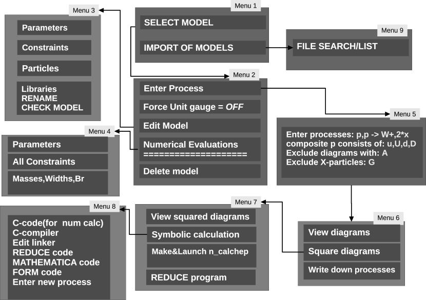
3 Interactive GUI symbolic session
The menu structure for the symbolic session of CalcHEP is shown schematically in Fig. 1. These menus allow the user to:
-
1.
select a model or import a new model from the file system [Menu 1].
-
2.
implement changes in a model [Menu 2,3] and check for syntax errors.
-
3.
set a flag which forces a calculation to be performed in physical (unitary) gauge for a model which has been written in t’Hooft-Feynman gauge [Menu 2];
-
4.
check numerically the mass spectrum, dependent parameter values and particle decay modes before generating a process [Menu 4];
-
5.
enter a scattering or decay process by specifying incoming and outgoing particles where decay processes and scattering processes are supported [Menu 2,5];
-
6.
generate Feynman diagrams, display them, optionally exclude diagrams as well as create the corresponding LaTeX output [Menu 6];
-
7.
generate, display and optionally exclude squared Feynman diagrams as well as create the corresponding LaTeX output [Menu 7];
-
8.
calculate analytic expressions for squared matrix elements by using the fast built-in symbolic calculator [Menu 7];
-
9.
export the symbolic expressions of the squared diagrams in REDUCE, MATHEMATICA or FORM format for further symbolic and/or numerical manipulations [Menu 7,8];
-
10.
generate optimized C code for the squared matrix element for further numerical calculations [Menu 8];
-
11.
launch the compilation of the generated C code and start the corresponding numerical session [Menu 8];
Many new features have been added to the symbolic session compared to version 2.3 [19]. They are:
-
*
The option to evaluate the processes is now available. It requires the distribution functions to be used for the incoming particles in the numerical session.
-
*
CalcHEP supports collision processes with polarized massless fermions and vector bosons in the initial state. This is accomplished by ending the particle’s name with a
%as in:e%,A%->e,Z -
*
CalcHEP now supports particles with spin up to 2 (including s= 0, 1/2, 1, 3/2 and 2).
-
*
A new column has been added to the particle table allowing to enter an ID for the particle from the Monte Carlo numbering scheme[41]. This ID is used to interface the model with parton structure functions, such as CTEQ and MRST, and with Monte Carlo packages such as PYTHIA[42]. In other words, this ID allows to interface a CalcHEP model with a package that uses the Monte Carlo ID and is independent of the names given to the particles. CalcHEP does a basic sanity test on the Monte Carlo ID’s given to particles to make sure they do not clash with the ID’s of existing mesons and baryons from the PDG. This helps avoid potential problems with hadronization and fragmentation when the CalcHEP events are being passed to external MC generators.
-
*
CalcHEP includes the SLHAplus package [34] and its functions can be used in CalcHEP model constraints. It allows to
- -
-
-
implement tree level calculations for particle spectra and mixing matrices for any field multiplet;
-
-
include QCD Yukawa corrections for Higgs-q-q vertices for correct Higgs width calculations;
Further details can be found in Section 9.1.
-
*
In the current CalcHEP version, we have added calculations for the Higgs-- and Higgs-gluon-gluon effective couplings to the SLHAplus routines. See section 9.2 for further details.
-
*
The width of a particle can now be calculated automatically during a numerical evaluation when the parameters change. To use this feature, the user must add a
!to the beginning of the width name in the particle table. For example, to activate automatic calculation of the Higgs boson’s width, the user should specify this in the particle table in the following wayFull name |A |A+ |PDG number |2*spin| mass |width |color|aux| Higgs |h |h |25 |0 | Mh |!wh |1 | |
The exclamation mark before the width symbol forces the width to be calculated automatically. CalcHEP does this by sequentially calculating the , , and processes until a non-zero value for the width is obtained. By default the decay processes are accompanied with and ones with virtual W and Z bosons. A proper matching with on-shell W/Z is done. This is important for a correct calculation of the Higgs widths as well as for some BSM particles. In Section 9.2, we present a comparision of branching fractions of Higgs decays obtained with the Hdecay program and CalcHEP. Calculation of channels with virtual W/Z can be switched off via the
F5function key. -
*
CalcHEP has an option to use particle widths calculated by an external package. If a CalcHEP model loads (in the
Constraintstable) a file with a SLHA decay table (see Sec.9.1), then the automatic width calculation presented above uses the values read from the SLHA file instead of an internal matrix element calculation. This behavior can be further controlled using an option to read or discard the widths from an SLHA file (see Section 9.1). Also width parameters can get SLHA values using SLHAplus functions explisitely [34]. -
*
Although SLHAplus contains many useful functions for model implementation, we foresee the need to link external packages and user written code to CalcHEP. This can be done in the new model table Libraries [Menu 3] and greatly enhances the facilities of CalcHEP. The user simply enters the path to the compiled code to be linked when generating
n_calchep. The Libraries table also allows the user to define prototypes of external functions. Two important uses for this functionality is to link the LHAPDF[45] structure function sets and user defined functions for phase space cuts and histograms. See the details in Sections 4.5 and 8.5. -
*
The
Numerical Evaluationsmenu [Menu 4] allows to evaluate the dependent parameters (constraints) as well as the widths and branching ratios of the particles before generating the code for a specific process. Like the automatic width calculation, it uses the dynamic linking facilities of modern operation systems. During this procedure, the decay processes are compiled when they are needed and stored in the directory$WORK/results/auxfor subsequent usage until the model is changed. - *
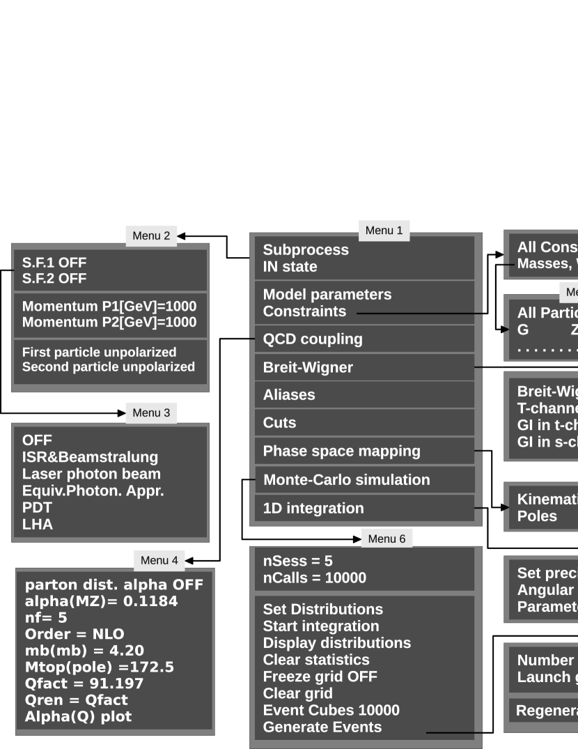
4 Interactive GUI numerical session
The menu system for the interactive numerical session GUI of CalcHEP is schematically presented in Fig. 2. It allows the user to:
-
1.
select a subprocess for numerical processing if the generated code contains more than one;
-
2.
set the momenta and helicities of incoming particles. The helicity is defined with respect to the direction of motion. For the electron it is in the interval []. A positive value (e.g. ) corresponds to a right-handed electron [Menu 1,2];
-
3.
convolute the squared matrix element with structure functions and beam spectra. CalcHEP comes with a set of parton distribution functions for protons and anti-protons, initial state radiation and beamstrahlung spectra for electrons, and the laser photon spectrum, Weizsaecker-Williams photon structure functions and proton photon structure functions for the photon [Menu 3]. The user also has the option to use the LHAPDF structure functions (see Sections 4.1 and 8.5 for details). We note that the contents of this menu depend on the particle ID (see Section 8.3) and not on the particle’s name;
-
4.
modify independent physical parameters such as the coupling constants and masses which are involved in the process [Menu 1]. These parameters can be changed one by one or the user can read the parameter values from a file using this menu. The file must contain one parameter on each line of the file with the parameter name on the left and the numerical value on the right separated by whitespace. For example,
Mh 125
-
5.
view masses and dependent parameters (constraints) [Menu 1]. The list of dependent parameters which appear in this menu depends on whether they have been set to be “public” in the model files (see Section 8.2);
-
6.
calculate and view particle widths and decay fractions. This can be done via the
Constraintsitem of [Menu 1]. This menu also allows to write the full list of particle masses, widths and branching ratios to a file in SLHA format; -
7.
choose the scale used in the evaluation of the QCD coupling constant and parton structure functions [Menu 4]. We also provide the user the option to define the normalization and factorization scales independently.
-
8.
apply various kinematical cuts [Menu 1 - Cuts option];
-
9.
define the kinematic scheme (phase space parametrization) in order to improve the efficiency of the Monte Carlo (MC) integration and also to introduce a phase space mapping in order to smooth the sharp peaks of a squared matrix element and structure functions [Menu 1 - Phase space mapping option];
-
10.
perform a Monte Carlo integration of the phase space by VEGAS [Menu 1,6] (see Section 4.7);
-
11.
generate partonic level events [Menu 1,6,7] (see Section 4.7);
-
12.
set and display distributions of various kinematical variables. It is also possible to export the distribution to file for use in external programs such as LaTeX, gnuplot, PAW and Mathematica [Menu 6];
4.1 Built-in and LHAPDF parton distribution functions
CalcHEP comes preinstalled with several parton distribution function sets
These sets and tools for updating them have been described in
[19]. To use one of these built-in PDFs, the user
should choose the PDT
(Particle Distribution Tables) item of Menu 3.
A more comprehensive set of PDFs
is available in the LHAPDF [45] library
which the user can install separately and link to a CalcHEP model by
using the Libraries model table.
The source code for LHAPDF can be downloaded from the URL:
http://projects.hepforge.org/lhapdf/
which also contains instructions for the installation of LHAPDF. To use the LHAPDF parton distribution functions in CalcHEP, the user should add the line
-L<path_to_lhapdf> -lLHAPDF
to the Libraries model table.
This is sufficient to generate and compile the code for a process
which creates the executable $WORK/results/n_calchep.
However, it may not be sufficient to launch it.
If libLHAPDF.so is located in a system area such as
/usr/lib, then the library will be detected automatically.
Otherwise, information about the location of the shared library needs
to be provided with environment variables.
We recommend to add the instructions
export LD_RUN_PATH=<path_to_lhapdf>
to the calchep script in the $WORK directory and
export LD_LIBRARY_PATH=$LD_LIBRARY_PATH:<path_to_lhapdf>
to the calchep_batch script in the same directory where
<path_to_lhapdf> is the path to the LHAPDF library.
By setting LD_RUN_PATH in the calchep script,
the user does not need to set this environment variable again before
starting the generated
n_calchep later. Also, using
LD_RUN_PATH in the calchep script allows the LHAPDF
library to be updated without the user recompiling
n_calchep.
If the linking of LHAPDF is successful then the LHA item will appear
in Menu 3.
4.2 SLHA formatted files
The Constraints menu allows the user to generate a complete SLHA file with all the particle’s properties for a model including the particles’ masses, widths and branching ratios. Since this file is is generate in SLHA format, the resulting file can be used by external programs such as MC generators.
To create this SLHA file,
the user should choose the Constraints option of Menu 1,
go to the Mass, Widths, Branching submenu [Menu 10] and then choose the
All Particles option [Menu 11].
When this option is chosen,
CalcHEP calculates the widths and branching ratios for the particles
and writes all the information in the SLHA file.
When it is finished, CalcHEP displays the meassage
See results in file ’decaySLHA_n.txt’
on the screen, where n is an integer.
We note that these SLHA files can also be created during the symbolic
session through the All Constraints menu item (Menu 4 of Fig. 1).
It is well known that for a correct calculation of the Higgs width and branching fractions, the QCD loop corrections must be included. This can be done by using running quark masses and yukawa couplings. In the default CalcHEP models, we include the following running quark masses which are coded in the SLHAplus package
McRun(Q) MbRun(Q) MtRun(Q)
and the effective quark masses
McEff(Q) MbEff(Q) MtEff(Q)
which depend on the QCD scale (Q) and should be used to calculate the
Yukawa couplings (in the Constraints table).
The effective masses calculated
at the Higgs mass scale provide the correct partial Higgs width at
NNLO. Parameters with the scale Q as an argument have a
special meaning in CalcHEP. When CalcHEP calculates the particle
width it substitutes the particle mass for the scale Q.
Further details can be found in [34].
To keep gauge invariance in tree level calculations, the particle’s pole mass must be the same as is used for the Yukawa coupling. For the c and b quarks, the effect is small at high energies. However, for the t quark the usage of the effective mass can lead to the wrong decay modes for BSM particles.
4.3 Built-in kinematical functions
CalcHEP has a wide set of built-in kinematical phase space functions which can be used to implement various kinematical cuts and/or to construct distributions 333We note that the user can also write his/her own routines for kinematical functions. Further details can be found in Section 4.5.. These functions are defined via the names of the outgoing particles and are called with the syntax
Name[^,_](P1[,P2,P3...]),
where Name is one capital letter specifying the function, the ^ and _
are optional function modifiers useful in the case of identical outgoing
particles (described below), and P1[,P2,P3...]
are the outgoing particles involved in the observable.
The available functions are:
-
A :
A(P1[,P2,...]) gives the angle between P1 and the combined momentum . If only one particle is specified, as in A(P1), the angle between P1 and the first incoming particle is returned. The angle is given in degrees.
-
C :
C(P1[,P2,...]) gives the cosine of the angle defined above for A(P1[,P2,...]).
-
J :
J(P1,P2) gives the jet cone angle between P1 and P2. The jet cone angle is defined as , where is the difference in pseudo-rapidity and is the difference in azimuthal angle between P1 and P2.
-
E :
E(P1[,P2,...]) gives the energy of the combined momentum .
-
M :
M(P1[,P2,...]) gives the invariant mass of the combined momentum .
-
P :
P(P1,P2[,P3,...]) first boosts into the cms frame of P1,P2[,P3,...] and then takes the cosine of the angle between P1 (in the cms frame) and the boost direction.
-
T :
T(P1[,P2,...]) gives the transverse momentum of the combined momentum .
-
Y :
Y(P1[,P2,...]) gives the rapidity of the combined momentum .
-
N :
N(P1[,P2,...]) gives the pseudo-rapidity of the combined momentum .
-
W :
W(P1[,P2,...]) gives the transverse mass of the particle set P1,P2,... given by
where and are the mass and transverse momentum respectively of the th particle.
For example, M(m,M) returns the invariant mass of a ,
pair.
In situations where there is more than one identical outgoing particle,
all permutations of that particle are tested for cuts while their histograms are
added. For example, suppose we have the process
where is a jet. The cut J(j,j) would be applied
to all six possible combinations of the three jets.
On the other hand, if this observable
were used for a distribution, each of the six combinations
would be binned for the histogram. In other words, the histograms for
each combination are added together. On the other hand, each particle is only used once
for each observable. So, for example, J(j,j) is never the jet
cone angle of a jet and itself.
The optional modifiers ^
and _ select the maximum and minimum value for the kinematical
function among all permutations. For example, J_(j,j)
calculates the jet cone angle of all pairs of jets and returns the
smallest one for the cut or histogram.
Although the momenta of incoming particles can not be measured directly,
distributions of these momenta can still be interesting and useful to
understand the details of the collision.
For this, E1 and E2can be used for the energy of the
first and second incoming particle, respectively. The total partonic
CMS energy can be obtained with M12.
4.4 Aliases
Aliases can be defined (see Menu 1 in Figure 2) for particle sets which will be substituted in the kinematical functions presented above. The user should enter each alias on a separate line where the name of the alias belongs in the first column and the particles that are contained in the alias belong in the second column. For example, a jet could be defined as:
   Name | Comma separated list of particles
   j    |u,U,d,D,c,C,s,S,b,B,G
in the default SM. A positively charged lepton of first or second generation might be defined as:
   Name | Comma separated list of particles
   l+   |E,M
in the default SM. The user can make any alias definitions
he/she likes as long as the names do not match any particle names.
These aliases can be used in the cuts and distribution definitions.
For example, a cut can be placed on QCD quarks and guons with one
line using an alias (T(j) rather than specifying a separate cut for each
quark and guon.
Note that all particles included in an alias are treated in the same manner as
identical particles. So, all combinations are tested for cuts and binned
for histograms.
4.5 User defined kinematical functions
To implement a new observable for cuts and distribution one can
write a usrfun routine which should be a C-code function.
The code of this function can be linked to the numerical session by
adding it to the CalcHEP model Libraries
table. The user can then call these observables as Ucode where
code is a user-defined string which is passed to the
usrfun routines for processing. These user-defined observables
can be used in cuts and
distributions. The full prototype of the usrfun function is
double usrfun(char *code, int nIn, int nOut, double *pvect, char **pName, int *pdg);
where
-
-
nInis the number of incoming particles. -
-
nOutis the number of outgoing particles. -
-
pvectis an array containing the momenta of the incoming and outgoing particles. The momentum of the particle (qi) where goes from to is given byqi[k]=pvect[4*i+k]where
kgoes from 0 to 3.qi[0]=pvect[4*i]gives the energy (which is always positive),qi[3]=pvect[4*i+3]gives the component of the momentum along the axis of collision andqi[1]andqi[2]give the transverse components of the momentum. -
-
pNameis an array of strings which contain the names of the particles.pName[0]gives the name of the first incoming particle,pName[1]gives the name of the second incoming particle,pName[2]gives the name of the first outgoing particle, and so on. -
-
pdgis an array of PDG ID codes for the particles.
Some further functions which the user may find helpful are:
    int findval(char *name, double *value);
    int qnumbers(char *pname, int *spin2, int *charge3, int *cdim);
The first accepts a parameter name (independent or dependent) and fills the value of the parameter. The second accepts a particle name and fills the quantum numbers of the particle. Further details of these functions can be found in Section 10.
We provide an example usrfun routine in the file
$CALCHEP/utile/usrfun.c
which calculates the transverse mass of two particles.
4.6 Cuts and distributions
The Cut item of Menu 1 allows the user to apply cuts to the
current process. This is done by filling in the cuts table with the
kinematical function (second column), the minimum limit for the cut
(third column) and the maximum limit for the cut (fourth column). The
minimum and maximum limits for the cut should be algebraic functions
of the model parameters and numbers. One of the limits can be left
blank, in which case that limit is not applied. If there is an
exclamation mark (!) in the first column, the cut is inverted.
For example
  ! |Parameter   | Min bound   |Max bound
    | M(b,B)     | Mh/2        | Mh*2
means that the invariant mass of a b-quark and an anti-b-quark must be between half the Higgs mass and twice the Higgs mass.
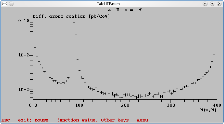
The syntax for the distribution table [Menu 6] is similar to that of the cut table.
Both one- and two-dimensional distributions are supported.
The distributions are filled during Monte Carlo integration and can be
viewed graphically with the Display distribution item of Menu 6.
An example of a distribution in the GUI is presented in
Fig. 3.
These distributions can be saved in a few different formats. The
first is to the file plot_n.txt where n enumerates the
plot files. This file has the data in two space separated columns.
It also contains example instructions at the top for using this file with PAW and
Gnuplot.
The data in these files can be re-displayed later by CalcHEP by the
plot_view routine as in
$CALCHEP/bin/plot_view plot_N.txt
The Clear Statics function of Menu 6 resets all the data.
We note that the kinematic functions used in the Cut and Distribution tables can
contain particles which are not present in the current
subprocess. When this occurs, these cuts are ignored and these
distributions are not filled.
In this way, cuts and distributions can be defined once for all
subprocesses. When a different subprocess is chosen [Menu 1], the
cuts and distributions that apply are automatically turned on.
4.7 Monte-Carlo simulation and event generation
CalcHEP uses VEGAS [46, 47] for Monte Carlo integration.
The Start Integration function of Menu 6 launches a cycle of NSess VEGAS
sessions with nCalls integrand calls for each session. If the switch
Freeze grid = OFF, VEGAS improves the integration grid
after each session444The importance sampling algorithms is used here..
Table 1(left) presents an example of a Vegas
session with the grid being improved as evidenced by the steep decline
in the Monte Carlo uncertainty in the Error column.
Although the grid is improved by the end of the session, the final
uncertainty (in the final line) is still large because it includes the
results of all ten sessions, including the initial sessions when the
grid was not yet improved. It is a good idea to clear the
results once the grid is improved and rerun VEGAS. This is done by using the
Clear statistics menu item and then Start Integration
again. An example of a VEGAS session after the grid has been improved
and the statistics cleared is shown in Table
1(right). The Monte Carlo uncertainty is small
for all ten sessions and the resulting cross section has a
correspondingly small uncertainty.
| IT | Cross section[pb] | Error[%] | nCalls | IT | Cross section[pb] | Error[%] | nCalls | Eff. | ||
|---|---|---|---|---|---|---|---|---|---|---|
| 1 | 1.8319E+00 | 1.29E+01 | 9826 | 1 | 2.0516E+00 | 2.33E-01 | 9826 | |||
| 2 | 2.0575E+00 | 5.76E+00 | 9826 | 2 | 2.0587E+00 | 2.27E-01 | 9826 | 8.5E-01 | ||
| 3 | 1.9409E+00 | 4.88E+00 | 9826 | 3 | 2.0506E+00 | 2.27E-01 | 9826 | 7.5E-01 | ||
| 4 | 2.2081E+00 | 6.63E+00 | 9826 | 4 | 2.0450E+00 | 2.28E-01 | 9826 | 7.1E-01 | ||
| 5 | 2.0717E+00 | 2.44E+00 | 9826 | 5 | 2.0511E+00 | 2.27E-01 | 9826 | 6.9E-01 | ||
| 6 | 2.0588E+00 | 7.72E-01 | 9826 | 6 | 2.0549E+00 | 2.26E-01 | 9826 | 6.7E-01 | ||
| 7 | 2.0624E+00 | 3.93E-01 | 9826 | 7 | 2.0623E+00 | 2.29E-01 | 9826 | 6.6E-01 | ||
| 8 | 2.0501E+00 | 2.81E-01 | 9826 | 8 | 2.0610E+00 | 2.28E-01 | 9826 | 6.5E-01 | ||
| 9 | 2.0472E+00 | 2.48E-01 | 9826 | 9 | 2.0516E+00 | 2.31E-01 | 9826 | 6.5E-01 | ||
| 10 | 2.0547E+00 | 2.24E-01 | 9826 | 10 | 2.0564E+00 | 2.27E-01 | 9826 | 6.4E-01 | ||
<> |
2.0383E+00 | 1.58E+00 | 98260 | 0.9 | <> |
2.0543E+00 | 7.23E-02 | 98260 | 6.4E-01 | 1 |
When Freeze grid = ON [Menu 6], VEGAS will prepare the event
generator during the VEGAS sessions. With each VEGAS pass, the event
generator will improve its estimates of the maximum differential cross
section (or differential partial width) in each event generation
cube. The number of event generation cubes can be set with the
Event Cubes item of [Menu 6] as in
     Freeze grid = ON
     Event Cubes  10000
The larger the number of event
cubes, the longer it takes to improve the event generator but the more
efficient the generator. In each cube, the maximum value will be set
at times the largest differential cross section (or differential
partial width) that VEGAS finds. Since with each pass the estimates
for the maximums will become larger (as VEGAS finds higher
values), the event generator efficiency will become smaller. The
event generator is prepared when the efficiency stabilizes. An example
of event generator preparation is shown in Table
1(right), where the Eff column gives the
estimated efficiency of the event generator after each VEGAS session.
The event generator preparation in the above paragraph is based on the
Von Neumann algorithm (see [41], p.202) where
a phase space point is sampled with a probability
(where in our case is the maximum deteremined during the event generator preparation) and
accepted with probability (where for us is the
differential cross section or partial width at ).
However, because the maximums are determined by the calculation of
random phase space points (by the VEGAS Monte Carlo), there are times
when will occur during event generation.
If CalcHEP finds such a point , it will increase for the
the rest of the event generation.
Furthermore, if Regenerate events [Menu 7] is set to
OFF, CalcHEP will accept this event and give it the weight
. On the other hand, if Regenerate events is set
to ON, CalcHEP will regenerate all the events from that event
cube.
When CalcHEP is finished generating the requested events, it will
display information about the events on the screen as in
          Event generated: 10000
            efficiency:  6.4E-01
       Max Event multiplicity: 2
       Multiple events(total): 3
including whether events with weight greater than 1 were generated and request whether the user would like to accept the generated events.
5 Working with files from numerical session
5.1 File naming convention
CalcHEP keeps an internal counter of numerical sessions. Any time a
parameter is changed that affects the numerical results,
CalcHEP increments the session number. All the parameters as well as
the state of the random number generator and the integration results
are stored in the file $WORK/results/session.dat. This allows
the numerical session to be run later starting from the same state.
The session number is displayed on the screen in the GUI.
Furthermore, the session number is used in the names of some files
written by CalcHEP in order to connect them with a particular
session. These files are
-
1.
prt_Nwhich contains complete information about the session parameters (including model parameters, momenta, structure functions, cuts, etc.) as well as some of the results from the VEGAS session; -
2.
decaySLHA_Nwhich contains information about the particle spectrum of the model and includes the particles’ decay channels in the format of [43] -
3.
distr_Nwhich contains the full distribution data filled by VEGAS which can be viewed later as described in Section 5.2; -
4.
events_N.txtwhich contains the generated events;
where N is the session number.
5.2 Distribution files
The distributions generated by CalcHEP can be displayed after a numerical session has finished with the command
$CALCHEP/bin/show_distr distr_N
where N is the session number where the distribution was generated.
The distributions generated in different numerical sessions can be
combined by the command
$CALCHEP/bin/sum_distr distr_A distr_B ... > distr_sum
where distr_A, distr_B ... are the distribution files from
different sessions and distr_sum is the file where the results
should be written.
This program only combines distributions with exactly the same
kinematical variable and exactly the same distribution limits. For
example,
M(b,B) and M(B,b) are treated as different
distributions are never summed.
However, the distribution M(jet,jet) where the alias name
jet has been defined appropriately (see Section 4.4) are combined if their
distribution limits are identical as well.
5.3 Events
CalcHEP writes events in the format presented in [1]. However, the the LHE format [48] has become widely used now. For this reason, we include a script to rewrite event files in LHE format which can be run as in:
$CACLHEP/bin/event2lhe events_N.txt > events_N.lhe
where N is the session number for the generated events.
Additionally, CalcHEP has routines to read the event files and
histogram the events. The notation for the kinematical observables is
the same as in Section 4.3. These routines can be run as
in the following examples:
       $CALCHEP/bin/events2tab Variable Min Max Nbin < events.txt > tab.txt
       $CALCHEP/bin/lhe2tab    Variable Min Max Nbin < events.lhe > tab.txt
where Variable is the kinematic observable and must be in
quotation marks (e.g. "M(m,M)"), Min and
Max are the histogram’s minimum and maximum values respectively, Nbin
is the number of bins, events.txt and events.lhe are the
event files in original and LHE format respectively and tab.txt
is the file where the results should be written.
In the case of the lhe2tab, the PDG ID’s of the particles
should be used in place of the particle’s names since the particle
names are absent in the LHE format.
The resulting histograms can be displayed on the screen and transformed into
PAW, Gnuplot, Mathematica and LaTeX formats by the plot_view routine.
For further analysis CalcHEP contains a program that creates PAW
NTUPLES from LHE files which is used in the following way
$CALCHEP/bin/nt_maker events.lhe
where events.lhe is an event file in LHE format.
5.4 Event Mixing and LHE format
Typical collider processes contains many subprocesses that differ only by the initial state and/or final state
particles. For example, at the LHC, the initial states are two
colliding protons which, however, are composed of quarks, antiquarks
and gluons. It is desirable to combine different channels in one event file and connect
production events with decays so that the final events are fully or
partial decayed. The CalcHEP routine which does this job is event_mixer and can be used as in
$CALCHEP/bin/event_mixer Lumi Nevent dir1 dir2 ...
where Lumi is the maximum integrated luminosity (in units of ), Nevents is the number of events to generate, and dir1 dir2 ... are the directories where the production and decay events are stored. If Nevents is smaller than Lumi times the final cross section (we will call this ), then Nevents will be produced. If, on the other hand, Nevents is larger, then event_mixer will stop when it reaches .
If event_mixer comes to the end of a decay file before it is finished producing the requested number of events, it prints a message to stderr and returns to the beginning of the decay event file.
The resulting events are stored in th file event_mixer.lhe in LHE format
[48].
Before event_mixer begins combining events, it reads the file decaySLHA.txt which should be stored in the current
directory. This file should contain the quantum numbers, masses, widths and branching ratios of the particles of the model
written in SLHA format [43]. This file is used to define the
correct widths and branching ratios of the decaying particles.
If this file is not present, event_mixer will determine the
branching ratios from the decay event files that it uses. However,
please note that if decaySLHA.txt is not present and all the
decay channels for an unstable particle are not present,
event_mixer will likely produce incorrect results.
The
decaySLHA.txt file can be produced by the CalcHEP numerical
session (see Section 4.2). We strongly recommend to always include it when using event_mixer.
After reading decaySLHA.txt but before combining events, event_mixer prints to stdout the final cross
section and the maximum number of events that can be generated. For example,
2.368E-01  -total cross section[pb]
10098      -maximum number of events
To get this information before mixing the events, simply request events.
Some special features of LHE file generated by CalcHEP are:
-
1.
The decays are applied recursively.
-
2.
A decay history of each event is stored in the LHE file. This includes information about the parent particles and their mean life time. This information can be used for proper hadronisation and detector simulation.
-
3.
When connecting decays,
event_mixeruses a Breit-Wigner virtual mass distribution, where we assume that the matrix elements of the subprocesses do not depend strongly on the off-shell momentum. -
4.
If
decaySLHA.txtfile was detected it is attaches to the output inside<slha> ... </slha>tags according to the LHE convention. This allows parton shower generators like Pythia and Herwig to implements the decays of BSM particles. -
5.
In case of an incomplete set of decay channel event files (which is detected via a difference between the sum of the partial widths from the decay event files and that stored in
decaySLHA.txt) the resulting cross section is reduced correspondingly. -
6.
In spite of Breit-Wigner mass smearing for decays our procedure does not break momentum conservation. The output file contains a line which records the largest deviation from energy momentum conservation. An example is
#lost_momenta_max/Etot 7.9E-11 1.3E-12 1.3E-12 8.0E-11
Typical value should be on the order of since the original event files contain 11 digits Of precision for the particle momenta.
The generated event_mixer.lhe file also contains
an XML header spanned by the tags <hepml> ..</hepml> written in HepML [49]
format. This allows to automatically upload the LHE file to the
CERN Monte-Carlo Database (MCDB) using the command555 The upload2mcdb_hepml.pl script can be downloaded from
the MCDB website https:\\mcdb.cern.ch.
./upload2mcdb_hepml.pl -header hepml event_mixer.lhe
If the file run_details.txt is found in the current directory,
event_mixer will include the information in this file in the
header. The format for this file is a keyword value pair on each
line and is the same as the format for a batch file used with the
batch interface. Further details can be found in Section 6.
6 CalcHEP blind mode and batch scripts
Initially CalcHEP was designed for interactive calculations with a graphical user interface. However, there are times when a batch system is ideal. For example, when a calculation takes a very long time, or the user is interested in doing scans over parameter space or over subprocesses.
In order to solve this problem, the blind mode was introduced
[50, 19]. If the -blind flag is used
with either s_calchep or n_calchep, they will read the
next argument and interpret it as a series of commands. These
commands are written in a special notation which matches the
keystrokes the user would perform during an interactive session. For
example, the command666One has to remove tmp/safe file before
launching this command.
$CALCHEP/bin/s_calchep -blind "fStandard Model{{{e,E->m,M{{[{[{{0"
would generate the C code for the process e,E->m,M
in the Standard Model.
Some of the characters in the command string have a special meaning.
Here are a few of them:
] |
-Up | } |
-Escape |
[ |
-Down | f |
-find or search for the string in a menu |
{ |
-Enter | 0-9 |
-Function keys or numeric input according to context |
Determining an appropriate command sequence string can be difficult
for a user. For this reason, both s_calchep and
n_calchep can be run with the flag +blind. In
+blind mode, the interactive graphical interface opens and the user can run
them as usual. When the user quits, CalcHEP writes the command
sequence string to stdout. The user can then copy it and modify as
appropriate to use in -blind mode.
Further technical details
can be found in [50, 19].
The -blind mode was used to write
several scripts which are stored in the $CALCHEP/bin directory. First of all, there are several scripts which change the
parameters of a
numerical session:
set_momenta p1 p2: This script updates the
momenta of the incoming particles to p1 and p2 and
then quits.
set_param name1 value1 name2 value2 ...: This
script changes the numerical values of one or more of the independent model
parameters name1, name2, etc. to value1,
value2, etc. respectively and then quits.
set_param File: In this case, this script
changes the numerical values of the independent model parameters
as specified in the file File. File must have each
model parameter on a separate line with the name coming first
followed by the new numerical value, separated by white space.
set_vegas nSess1 nCalls1 nSess2 nCalls2 EventCubes :
This script sets the parameters of a two loop Vegas calculation
used by the
run_vegas script presented below. The meaning of the
parameters was explained in Section 4.7. They can be seen in
Fig.2. The statistics are cleared and the grid is frozen between session
1 (defined by nSess1 and nCalls1) and session 2
(defined by nSess2 and nCalls2).
The full set of parameters for the numerical session are stored
in the file session.dat. When the interactive GUI session
(n_calchep) runs or when any of these scripts run, they update
session.dat with the new parameters before quitting. As a
result, when the interactive GUI session (n_calchep) or these
scripts are run later, they begin with the updated parameters of the
last session. This allows the user to prepare for a blind calculation
in two ways. The user can either run the interactive GUI session
(n_calchep) and set all the parameters as needed or he/she can
run these scripts to set the parameters as required. Once the
parameters are set appropriately, the folowing scripts allow to run
VEGAS:
run_vegas:
This script runs VEGAS according to the parameters in session.dat.
There are several scripts which perform scans which are based on
run_vegas. The output for these cycles is stored in text files whose names
have the form xxx_j1_j2, where j1 is
the session number when the script began and j2 is the session number when it
finished. If there are distributions specified in session.dat,
they are stored in the files distr_k where j1 k
j2. These scripts are:
pcm_cycle pcm0 step N: This
script scans the cross-section over the center of mass energy. For each point in the
scan, it updates the momenta of the initial state particles and then runs the Vegas Monte
Carlo integration. It begins its calculations with the momenta of the initial state particles
equal to pcm0 and increases in steps of size step for a total of N steps.
When it is finished, it writes the resulting cross-sections to the file
pcm_tab_j1_j2.
name_cycle name val0 step N: This script scans
the cross-section over a model parameter’s value. For each point in
the scan, it updates the parameter name and then calculates
the cross-section. When it is finished, it writes the resulting
cross-sections to the file name_tab_j1_j2.
where name is the name of the parameter.
subproc_cycle L Nmax: This script calculates
the cross-section and generates events for each subprocess. When it
is finished, it adds the cross-sections together and prints the
total cross-section to the screen. If there are distributions
specified then they are added together and the resulting distribution is
stored in the file distr_j1_j2. It
also generates unweighted events for each subprocess. The number
it generates is equal to the smaller of Nmax and the cross-section times the luminosity
which is specified by L. It writes these
events to the files events_k.txt where j1 k j2.
par_scan < data.txt: This script calculates
the cross-sections according to the grid for names and parameters
given in data.txt file. The format of data.txt
is
  name_1  name_2 ... name_N
  val_11  val_12 ... val_1N
  .........................
  val_M1  val_M2 ... val_MN
where name_1 name_2 ... name_N are the names of independent model parameters
, while val_11 ... val_1N are the values for the respective
parameters to be used for the first calculation and
val_M1 ... val_MN are the values for these parameters for
the last parameter point to be calculated.
Note that this script does not sum over the subprocesses
(i.e. it will do the calculation only for the subprocess currently
chosen in session.dat).
The results of the calculations are printed to stdout and can be
redirected into a file with a command such as
par_scan < data.txt > results.txt
where results.txt is the file where the results should go.
The output format repeats the input format but contains one
additional column with the results of the calculation.
par_scan_sum < data.txt: This script calculates
the cross-sections according to the parameter points in
data.txt similarly to par_scan. However, this script
calculates the cross section for all the available subprocesses and
sums them together.
gen_events Nevents: This script can by launched
after a successful VEGAS calculation including a session where the
grid is frozen to improve the event generation grid. This can be done
with the run_vegas script described in this section. The
argument Nevents defines the number of events to generate.
If any of these scripts ends with an error, a message is printed to
stderr and the return value of the script can be
seen by issuing echo $? on the shell. A description of the
possible error codes can be found in the CalcHEP manual.
7 Batch interface
Although the shell scripts of the previous subsection greatly improve the users ability to run their desired processes in batch mode, there are still some limitations when doing large complex calculations involving scans over parameter space, many subprocesses and parallelization. To overcome these challenges, we have written a Perl script which we call the “batch interface”. The main features of this Perl interface are:
-
1.
The input is a pure text file we call the “batch file”. It consists of a series of keywords together with values for those keywords, with each keyword on a separate line. Most of the options available in the interactive session are supported by keywords in the batch file and thus most calculations can be done using the batch interface.
-
2.
A library of subprocess numerical codes is utilized. Each time the batch interface is run, it first checks whether the subprocess numerical code exists. If it does, it reuses it and skips the often long process of code generation. Any requested numerical codes not in the library are then generated and added to the library. If the model changed, the numerical codes are regenerated as appropriate.
-
3.
The numerical phase space integration is done and events are generated for each subprocess and the results are combined. Production and decay events are connected and the final event output is an LHE file with all the events fully decayed which can be used directly by Pythia or other software.
-
4.
Multiple parameters can be scanned over. For each parameter point, the results are combined and stored with names unique to that parameter point for easy retrieval.
-
5.
Both the symbolic calculations and the numerical calculations are parallelized. Each subprocess and each parameter point are run as separate jobs and run on all available cpu cores. The number of cores available is set by the user as is the type of cluster software used. Multicore machines, PBS cluters and LSF clusters are currently supported.
-
6.
The progress of the calculation is stored in a series of html files which can be viewed in a web browser777The inspiration for creating html pages that showed the progress of the calculation was obtained from MadGraph [51].. These html pages contain information about the progress of the calculation as well as the results of the calculations which are already finished. The final event files are linked as are the session.dat and prt files which give the full details of each individual calculation. Pure text versions of the progress pages are also created for situations where a web browser is not convenient.
Once the user creates the batch file and runs the batch interface, no user input is required until it finishes. It can be run in the background and checked periodically.
After the user has created their batch file, they would typically run the batch interface from their CalcHEP work directory as
./calchep_batch batch_file
where batch_file is the name of their batch file, which can be
named anything the user likes. The batch interface will start by
printing a message to the shell which will contain the location of the
html progress reports which the user can simply copy and paste into
their browser url window. The first time the user runs the batch
interface, they can also run the following from the work directory
./calchep_batch -help
which will complain that no batch file was present, create a series of html help files and quit. The location of the html help files will be printed to screen. This html help file can be opened in a web browser and contains all the details that are presented here.
In the following subsection we describe each keyword available
for the batch file and how to use it. An example batch file is stored
in CALCHEP/utile/batch_file.
7.1 Batch files
Comments
Any line beginning with a # is ignored by run_batch. The # has to be
at the very beginning of the line. Some examples are:
# This is ignored.
#Model: Standard ModelΨ This is ignored.
Model: # Standard Model(CKM=1) This is not ignored.
Model
The first section of the batch file should contain the specification of the model. This is done by model name and should match exactly the name in the CalcHEP model list. So, if you want to run the “Standard Model(CKM=1)”, you would specify this with the batch file line:
ModelΨ:ΨStandard Model(CKM=1)
There is no default for this line. It must be included.
The gauge of the calculation should also be specified in this section. Choices are Feynman and unitary gauge. CalcHEP is much better suited to calculation in Feynman gauge, but there may be times that unitary gauge is useful. This can be specified using the keyword Gauge as in:
GaugeΨ:Ψunitary
The default is Feynman.
CalcHEP allows decays of particle such as the Higgs boson via
off-shell W and Z bosons (see Section 1). This behavior can be controled by the key phrase Virtual W/Z decays as in:
Virtual W/Z decays : Off
The default is On.
Process
Processes are specified using the Process keyword and standard
CalcHEP notation as in:
ProcessΨ:Ψp,p->j,l,l
Multiple processes can also be specified as in:
ProcessΨ:Ψp,p->E,ne
ProcessΨ:Ψp,p->M,nm
As many processes as desired can be specified. When more than one process is specified, the processes are numbered by the order in which they are specified in the batch file. So, in this example, p,p->E,ne is process 1 and p,p->M,nm is process 2. This numbering can be useful when specifying QCD scale, cuts, kinematics, regularization and distributions allowing these to be specified separately for each process. There is no default for this keyword. It must be specified.
Decays are specified using the Decay keyword and are also in
standard CalcHEP notation as in:
DecayΨ:ΨW->l,nu
Again, multiple decays can be specified as in:
DecayΨ:ΨW->l,nu
DecayΨ:ΨZ->l,l
The default is to not have any decays. Cuts, kinematics, regularization and distributions do not apply to decays.
It is sometimes convenient to specify groups of particles as in the
particles that compose the proton or all the leptons. This can be done
with the keyword Alias as in:
AliasΨ:Ψp=u,d,U,D,G
AliasΨ:Ψl=e,E,m,M
AliasΨ:Ψnu=ne,Ne,nm,Nm
AliasΨ:ΨW=W+,W-
As many aliases as necessary can be specified. These definitions can be used in cuts and distributions as well as in the processes and decays. The default is not to have any alias definitions.
The PDF of a proton or antiproton can be specified with the
pdf1 and pdf2 keywords which correspond to the pdfs of
the first and second incoming particles respectively. Choices for
these keywords are:
   cteq6l (proton)         cteq6l (anti-proton)
   cteq6m (proton)         cteq6m (anti-proton)
   cteq5m (proton)         cteq5m (anti-proton)
   mrst2002lo (proton)     mrst2002lo (anti-proton)
   mrst2002nlo (proton)    mrst2002nlo (anti-proton)
   None
An example for the LHC is:
pdf1Ψ:Ψcteq6l (proton)
pdf2Ψ:Ψcteq6l (proton)
The default is None. These keywords can also be used for electron positron colliders. For this process the available pdfs are:
  ISR
  ISR & Beamstrahlung
  Equiv. Photon
  Laser photons
  None
The following proton electron collider pdf is also available:
-
1.
Proton Photon
All of these pdfs must be typed exactly or copied into the batch file.
If ISR & Beam is chosen, then the following beam parameters may
be specified:
Bunch x+y sizes (nm)Ψ:Ψ550
Bunch length (mm)Ψ:Ψ0.45
Number of particlesΨ:Ψ2.1E+10
The default values are the default values in CalcHEP and correspond roughly with the ILC.
If Equiv. Photon is chosen for the pdf, then the following
parameters may be specified:
Photon particleΨ:Ψe^-
|Q|maxΨ:Ψ150
Choices for the Photon particle keyphrase are mu^-,
e^-, e^+, mu^+. The default is e^+. The
default for the keyword |Q|max is the same as in the CalcHEP
interactive session.
If Proton Photon is chosen then the following may be specified:
Incoming particle massΨ:Ψ0.937
Incoming particle chargeΨ:Ψ-1
|Q^2|maxΨ:Ψ2.1
Pt cut of outgoing protonΨ:Ψ0.11
The defaults are the same as in the CalcHEP interactive session.
The user can also use PDFs from the SLHA library if it is installed
and the respective link is given in the model Libraries table.
Here is an example of how to use PDF functions from the LHAPDF library:
pdf1: LHA:cteq6ll.LHpdf:0:1
pdf2: LHA:cteq6ll.LHpdf:0:1
In this case, the value for pdf1 and pdf2 should be
constructed using the following rules:
1) It should begin with LHA.
2) LHA should be followed by the name of a particular PDF set
located in the PDFsets directory (e.g. cteq6ll.LHpdf in the example above).
3) The PDF set name should be follwoed by a particular PDF set number
(e.g. 0 in the example above corresponding with the central fit).
4) This should be followed by either 1 (for a proton) or -1
(for an antiproton).
5) The pieces from instructions (1)-(4) should be separated by a colon (:).
Momenta
The momenta of the incoming states can be specified with the keywords
p1 and p2 and are in GeV as in:
p1Ψ:Ψ7000
p2Ψ:Ψ7000
These are the default values for the momenta.
Parameters
The default parameters of the model are taken from the varsN.mdl file
in the models directory. Other parameter values can be used if
specified using the Parameter keyword. Here is an example:
ParameterΨ:ΨEE=0.31
This gives a convenient way of changing the default values of the parameters. Simply open CalcHEP in symbolic mode, choose to edit the model and change the values of the indepenedent parameters. These new values will then become the default values used by this batch program. There is no need to redo the process library.
Scans
In some models it is useful to scan over a parameter such as the mass
of one of the new particles. For example, if there is a new W’ gauge
boson, it may be desireable to generate events and/or distributions
for a range of masses for the W’. This can be done with the
Scan parameter, Scan begin, Scan step size and
Scan n steps keyphrases. Here is an example:
Scan parameterΨ:ΨMWP
Scan beginΨ:Ψ400
Scan step sizeΨ:Ψ50
Scan n stepsΨ:Ψ17
This will generate the events and/or distributions for the model with the mass of the W’ set to 400GeV, 450GeV, 500GeV,…1200GeV. As many scans as desired can be specified (including zero). For each scan, all four keyphrases have to be specified. Furthermore, if there is more than one scan, all four keyphrases have to be specified together.
QCD
The parameters of the QCD menu of the numerical session can be specified as in the following example:
parton dist. alphaΨ:ΨON
alpha(MZ)Ψ:Ψ0.118
alpha nfΨ:Ψ5
alpha orderΨ:ΨNLO
mb(mb)Ψ:Ψ4
Mtop(pole)Ψ:Ψ174
alpha QΨ:ΨM45
The default values are the ones in the interactive session. Not all the keywords have to be included in the batch file. It is sufficient to include the ones that need to be changed.
The QCD scale can be specified in terms of the invariant mass of
certain final state particles as in Mij which means that the
QCD scale is taken to be the invariant mass of particles i and
j. Or, it can be specified as a formula in terms of the
parameters of the model as in Mt/2 which means half of the top
quark mass. When specifying the scale in terms of the invariant mass
of final state particles, the numbers are taken from the way the
processes are entered with the Process keyword. So, if the
process is specified as p,p->j,l,n, M45 means the
invariant mass of the lepton and neutrino (l,n). The batch script will
take care of renumbering if the subprocesses have the final state
particles in a different order. It is also sometimes useful to use a
different scale for different processes. For example, suppose the two
processes p,p->j,l,n and p,p->j,j,l,n are specified in
the batch file, the scales could be specified as in this example:
alpha QΨ:1:ΨM45
alpha QΨ:2:ΨM56
The number between the :: specifies which process to apply this
scale and corresponds to the order in which the user specified the
processes. If more than one process is specified, but the same non
default scale is desired for all of them, this can be specified as in:
alpha QΨ:ΨMt/2
This specification will apply the same scale Mt/2 to all processes.
Cuts
Cuts are specified with the keywords Cut parameter,
Cut invert, Cut min and Cut max and use standard CalcHEP
notation, except for Cut invert which can be either True
or False. These cuts are only applied to the production
processes. They are not applied to the products of the decays. Here is
an example:
Cut parameterΨ:ΨT(le)
Cut invertΨ:ΨFalse
Cut minΨ        :Ψ20
Cut maxΨ        :Ψ
For each cut, all four keyphrases have to be present. As many cuts as
desired can be included. Including Cut min or Cut max
but leaving the value blank will leave the value blank in the CalcHEP
table. If the cut should only be applied to a certain process, then
the colon can be changed to :n: where n is the process
number.
Kinematics
As the number of final state particles increases, it can be very
helpful to specify the kinematics which helps CalcHEP in the
numerical integration stage. This is done in exactly the same notation
as in CalcHEP. The numbering corresponds to the order the particles
are entered in the process in the batch file. Here is an example:
KinematicsΨ:Ψ12 -> 34 , 56
KinematicsΨ:Ψ34 -> 3 , 4
KinematicsΨ:Ψ56 -> 5 , 6
If multiple processes are specified, using a single colon will apply the kinematics to all processes. If
different kinematics are desired for each process, then the :n:
notation can be used.
Regularization
When a narrow resonance is present in the signal, it is a good idea to
specify the Regularization. This is done with the same notation
as in CalcHEP. Here is an example:
Regularization momentumΨ:Ψ34
Regularization massΨ:ΨMW
Regularization widthΨ:ΨwW
Regularization powerΨ:Ψ2
Regularization for as many resonances can be specified as
desired. Furthermore, different resonances can be specified for each
process using the :n: notation.
Distributions
Distributions are only applied to the production process. The decays are ignored. Standard CalcHEP notation is used for the distribution parameter. Here is an example:
Dist parameterΨ:ΨM(e,E)
Dist minΨ:Ψ0
Dist maxΨ:Ψ200
Dist n binsΨ:Ψ100
Dist titleΨ:Ψp,p->l,l
Dist x-titleΨ:ΨM(l,l) (GeV)
The value for the keyphrase Dist n bins has to be one of
300, 150, 100, 75, 60, 50,
30, 25, 20, 15, 12, 10,
6, 5, 4, 3 or 2.
These are the values allowed by the CalcHEP histogram routines. The values given for the titles have to be pure text. No special characters are currently allowed. Gnuplot must be installed for plots to be produced on the fly and included in the html progress reports. More than one distribution can be specified. Also, distributions will work even if no events are requested.
For this to work, the distributions have to be unambiguous and apply to all subprocesses the same way. For example, if a process is p,p->l,l,l and the distribution M(l,l) is given, then this routine will not know which two leptons to apply the distribution to and the results are unpredictable. If the process is p,p->l,l where l=e,E,m,M and the distribution M(e,E) is desired, this distribution will only apply to some of the subprocesses and give unpredictable results. Make sure your distribution is unambiguous and applies in exactly one way to each subprocess. If this is done, it should work. Nevertheless, check each distribution carefully to make sure it is being done correctly.
Events
The number of events is specified with the keyphrase
Number of events. This specifies the number of events to
produce after all subprocesses are combined and decayed. If a scan over
a parameter is specified, this keyphrase determines the number of
events to produce for each value of the scan parameter. The number of
events requested can be zero. In this case, the cross sections are
determined and the distributions generated but no events are
produced. Here is an example:
Number of eventsΨ:Ψ1000
The name of the file can be specified using the
Filename keyword. If specified, all the files will begin with
this name. Here is an example:
FilenameΨ:Ψpp-ll
If nt_maker has been installed in the bin directory, PAW
ntuples can be made on the fly by setting NTuple to True
as in:
NTupleΨ:ΨTrue
The default is False.
The keyword Cleanup determines whether the intermediate files
of the calculation are removed. This can be useful if many large
intermediate files are created and space is an issue. On the other
hand, it can be useful to keep the files when debugging is necessary.
If this keyword is set to True, the intermediate files are
removed. If set to False then they are not removed. Here is
an example:
CleanupΨ:ΨFalse
Parallelization
The parallelization mode is set using the keyphrase
Parallelization method and can be either
local, pbs or lsf. In local mode, the jobs
run on the local computer, in pbs mode, the jobs are run on a
pbs cluster and in lsf mode, the jobs are run on an lsf
cluster. If run from a pbs or lsf cluster, the terminal should be on
the computer with the pbs or lsf queue. Here is an example of setting
the batch to run in pbs mode:
Parallelization modeΨ:Ψpbs
Local mode is the default.
If run in pbs mode, there are several options that may be
necessary for the pbs cluster. All of them can be left blank in which
case they will not be given to the pbs cluster. Here is an example of
the options available:
QueΨ:Ψbrody
WalltimeΨ:Ψ1.5
MemoryΨ:Ψ1
emailΨ:Ψname@address
The que keyword specifies which pbs queue to submit the jobs to. Walltime specifies the maximum time (in hours) the job can run for. If this time is exceeded, the jobs are killed by the pbs cluster. Memory specifies the maximum amount of memory (in G) that the jobs can use. If this memory is exceeded by a job, the pbs cluster will kill the job. email specifies which email to send a message to if the job terminates prematurely. The default for all of these is whatever is the default on the pbs cluster.
If run in lsf mode, there is one more option in addtion to the those above:
ProjectΨ:Ψproject_name
Sleep time specifies the amount of time (in seconds) the batch
script waits before checking which jobs are done and updating the html
progress reports. If a very short test run is being done, then this
should be low (say a few seconds). However, if the job is very large
and will take several hours or days, this should be set very high (say
minutes or tens of minutes or hours). This will reduce the amount of
cpu time the batch program uses. Here is an example setting the sleep
time to 1 minute:
sleep timeΨ:Ψ60
The default is 3 seconds.
When jobs are run on the local computer, the keyword Nice level
specifies what nice level the jobs should be run at. If other users
are using the same computer, this allows the job to be put into the
background and run at lower priority so as not to disturb the other
users. This should be between 0 and 19 where 19 is the lowest priority
and the nicest. Typically, it should be run at level 19 unless the
user is sure it will not disturb anyone. The nice level should be set
both for a local computer and for a pbs or lsf batch run. The reason
is that some jobs are run on the pbs or lsf queue computer even on the
pbs or lsf cluster. Here is an example:
Nice levelΨ:Ψ19
Level 19 is the default.
Vegas
The number of vegas calls can be controlled with the keywords
nSess_1, nCalls_1, nSess_2 and
nCalls_2. The values are the same as in CalcHEP. Here is an
example:
nSess_1Ψ:Ψ5
nCalls_1Ψ:Ψ100000
nSess_2Ψ:Ψ5
nCalls_2Ψ:Ψ100000
The defaults are the same as in CalcHEP.
Generator
The following parameters of the event generation can be modified:
sub-cubesΨ:Ψ1000
The defaults are the CalcHEP defaults.
Examples of batch files and the output results are given in section 11.
7.2 Monitoring batch session
The batch session is started with the command:
./calchep_batch batch_file
where batch_file is the name of the file that contains the
batch instructions. The batch program will print the following to
screen:
calchep_batch version vv

Processing batch:
Progress information can be found in the html directory.
Simply open the following link in your browser:
file:///WORK/html/index.html
You can also view textual progress reports in WORK/html/index.txt
Ψand the other .txt files in the html directory.
Events will be stored in the Events directory.
where vv is the version number and WORK denotes the path
to the calchep working directory.
The user can view the progress in their favorite browser as well as
check the results and details.
Examples of the different batch files and the resulting output
are given in Section 11.
Among the details of the resutls, the html pages contain links to the
prt_1 and session.dat files for each subprocess and each scan parameter. These
files contain the full details of the VEGAS session including all the
parameters of the run. At the bottom of the prt_1 file, there
is a history of the results of the VEGAS phase space integration. The
user may find these useful.
7.3 Results
After the events and/or distributions are generated, they are stored
in the Events directory. The prefix of the files is the name specified
in the batch file plus either -single if no scans were specified or
a string specifying the scan parameter values if one or more scans are
specified. We will assume this is filename in the following. If events
are requested, they will be stored in the files
filename.lhe.gz
filename.nt
where filename.lhe is the event file in Les Houches format and
filename.nt is in PAW ntuple format. The ntuple file is only
created if the keyword NTuple is set to True and
nt_maker is present in the bin directory. If distributions are
requested, they will be stored in the files
filename.distr
filename_1.png
filename_2.png
...
where filename.distr is the raw distribution data and can be read by show_distr in the bin directory. The distributions generated on the fly by the batch script are stored in the files ending in .png.
8 Particle interaction model implementation
A model of particle interaction in CalcHEP is stored in five tables, named Parameters, Constraints, Particles, Vertices and Libraries. These tables are stored in the respective files varsN.mdl, funcN.mdl, prtclsN.mdl, lgrngN.mdl, extlibN.mdl which are located in WORK/models/. The N in these file names refers to the model number. For all of these tables, a % at the beginning of any row means that that row is a comment and CalcHEP ignores it. We describe each of these tables in this section.
8.1 Independent parameters
The table Parameters contains all the independent parameters of the model. It consists of three columns, for example,
| Name | Value | Comment |
| EE | 0.3123 | elecromagnetic constant |
| SW | 0.481 | MS-BAR sine of the electroweak mixing angle |
| MZ | 91.187 | Z-boson mass |
| Mh | 125 | higgs mass |
where
-
Name:
This is where the name of the parameter belongs. It can contain up to 11 characters. The first character must be a letter. The others may be either letters or digits. The underscore symbol is also permitted and CalcHEP is sensitive to the case of the characters. There is a set of reserved names which cannot be used for parameter names:
-
(a)
i is reserved for the imaginary unit;
-
(b)
Sqrt2 is reserved for ;
-
(c)
p1,p2,p3,… are reserved for particle momenta;
-
(d)
m1,…,M1,… are reserved for Lorentz indices;
-
(e)
G5 is used for the Dirac matrix;
There is another subtelty that should be considered when naming parameters. Although CalcHEP is sensitive to the case of the parameters, Reduce is not. Therefore, if the user would like to use the CalcHEP results in Reduce, he/she should distinguish all names by more than case. Additionally, although CalcHEP allows underscores as part of parameter names, the underscore is treated differently by Mathematica. So, if the user would like to use the CalcHEP results in Mathematica, he/she should not use underscores in the parameter names.
-
(a)
-
Value:
This is where the numerical value for the parameter is stored. Dimensionful parameters should be in powers of GeV.
-
Comment:
This is where the user can enter a description of the parameter. It is ignored by CalcHEP and is purely for informational purposes.
There are two parameters which are treated specially in CalcHEP.
They are GG and Q. The first is reserved for the strong
coupling
CalcHEP forbids the appearence of this parameter in the Constraint table and in
the Lorentz part of the Vertices table (see below). But,
it can appear
in the Factor column of the Vertices table. This parameter is evaluated by
CalcHEP using QCD parameters which the user can view and/or modify in Menu 4 of
Fig.2. CalcHEP ignores the value of GG found
in the Paramters table. The variable Q is intented to be
used as a scale parameter in
the quark effective masses and Yukawa couplings. When CalcHEP peforms a
calculation of the particle width, it sets Q equal to the
decaying particle’s mass. This scale is then used to calculate the
quark effectifve masses at that scale (see Sections 4.2 and 9.1).
In all other cases, Q is set equal to its value from the Paramters table.
8.2 Dependent parameters
The Constraints table contains all the dependent parameters of the model. It consists of two columns, for example,
| Name | Expression |
|---|---|
| CW |
sqrt(1-SW^ 2) % cos of the Weinberg angle
|
| MW |
MZ*CW % W-boson mass
|
| GF |
EE^2/(2*SW*MW)^2/Sqrt2 % Fermi constant
|
| %Local! |
where
-
Name:
This is where the name of the parameter belongs. The restrictions on the names are the same as for the independent parameter names.
-
Express:
This is where the formula belongs which defines the value of this dependent parameter. The formula can contain the following:
-
(a)
integer and float point numbers,
-
(b)
independent parameter names contained in the Parameters table,
-
(c)
dependent parameter names defined above the current row,
-
(d)
parentheses
()and arithmetic operators+, -, /, *, ^, -
(e)
the symbols
iandSqrt2, -
(f)
standard functions from the C mathematics library such as
sqrt(x)andsin(x). The full list of these functions is contained in the $CALCHEP/include/extern.h file, -
(g)
functions from the SLHAplus package (see Section 9.1) which collects many routines useful for model building,
-
(h)
the function
if(x,y,z)which returnsyifxandzotherwise, -
(i)
any user defined functions. The code containing these functions should be included in the Libraries table. Their prototypes should also be included in the Libraries table. If their prototypes are not included, CalcHEP assumes they return double type. A list of the resulting auto-prototyped functions appears in the WORK/results/autoprot.h file after compilation of the numerical code.
-
(a)
Additionally, anything after the % symbol is considered a comment and ignored. This can be used to enter a comment about the dependent parameters.
Some models contain thousands of dependent parameters. For a particular process, only a small subset of these is used. To reduce the size of the generated code, CalcHEP compiles only the dependent parameters involved in the current matrix element calculation. However, it is sometimes necessary to have other dependent parameters compiled with the matrix element code in order to apply constraints such as on the particle spectrum. For this reason, CalcHEP splits all the dependent models parameters into two sets: the public parameters and the local parameters. By default, the public parameters are those that are required to calculate all the particle masses and widths as well as those that depend on external functions (except for dependence on standard C math functions) and all dependent parameters above any of these. All the dependent parameters below these are defined as local. The local parameters are not compiled unless they are needed for a matrix element calculation. If the user would like to force CalcHEP to include a larger subset of the dependent parameters in the numerical code, he/she can place the comment %Local! in the Constraints table in the first column. CalcHEP will always include the parameters up to, at least, this point.
The Constraints menu item of Fig. 2 displays only public parameters. These can be used along with global parameters in the specification of cuts and histogram limits, user-defined kinematical functions, and the QCD scale (see Section 4). The user-defined external functions can get the values of the independent model parameters and public dependent model parameters with the routine
int findval(char *name, double *value);
where name is the parameter name and *value is filled
with the value of the parameter. More details can be found in Section 10.3.
8.3 Particles
The particles are defined in the Particles table which consists of 11 columns. Each particle anti-particle pair is described by one row of the table. For example
| Full name | A | A | PDG | 2*spin | mass | width | color | aux | LaTex(A) | LaTeX(A+) |
|---|---|---|---|---|---|---|---|---|---|---|
| W-boson | W+ | W- | 24 | 2 | MW | wW | 1 | G | W^+ |
W^- |
| Higgs | h | h | 25 | 0 | Mh | !wh | 1 | h | h |
The columns are:
-
Full name:
The full name of the particle can be entered here. It is not used directly by CalcHEP. It is used to clarify what the short particle names mean.
-
A&Ac:
These columns are where the particle name and antiparticle name belong. More precisely, these columns contain the quantum field and its C-conjugate. The field operator acting on the vacuum is understood to create the corresponding anti-particle. Self-conjugate fields (such as photons and Majorana neutrinos) should contain the same name in both columns. Any printing character can be used in the particle name except white space, parentheses and the percent symbol (%). The length of the particle name can not exceed 8 symbols. For long particle names, we should note that the graphical representation of the diagrams might contain overlapping symbols.
-
PDG:
This is where the PDG code [41] belongs. This number is used mainly for interfacing with other packages. For example, these codes are included in event files [48] in order to communicate the particle flavor to other programs. The parton distribution functions are also applied according to this number. The conventional PDG codes should be used for SM particles. For other particles, the user should ensure that the code is not reserved for another particles such as a meson or baryon. Otherwise, conflicts could arise when passing events to other programs, such as Pythia.
-
2*Spin:
This is where the spin of the particle is specified. It should be entered as the integer equal to twice the spin. In other words, 0 should be entered for a scalar field, 1 for a spin fermion, 2 for a vector boson, 3 for a spin fermion and 4 for a spin-2 boson. Spin and particles should be massive.
-
Mass:
This is where the mass of the particle is entered. If massless, 0 can be entered. Otherwise, it must be a parameter name which is defined in either the Parameters table or the Constraints table.
-
Width:
This is where the width of the particle is entered. If the particle is stable, 0 can be entered. Otherwise, it must be a parameter name. In this case, however, this parameter can be defined in the Parameters table, the Constraints table or it can be preceeded with the ! symbol. If it is preceeded with the ! symbol, CalcHEP will automatically calculate it when needed. In this case, the parameter should not appear in either the Parameters table or the Constraints table. When automatically calculating the width, CalcHEP first attempts the decays. If none are found, it attempts the decays. If none are still found, it attempts the decays. If none are found at this point, it takes the width as zero. If information about particle widths was read from a SLHA file (See section 9.1), then the widths are not evaluated and CalcHEP substitutes the values it read from the SLHA file in the propagators.
-
Color:
This is where the color (SU(3)) representation is specified. Supported representations are the singlet (specified by a 1), the fundamental triplet (specified by a 3) and the octet (specified by a 8.) If the particle is specified as a triplet, the antiparticle is treated as an anti-triplet (the representation.)
-
Aux:
This field is primarily used to modify the propagator of the field. For most fields, this column will be left blank. The other possibilities are:
-
(a)
* : specifies that the propagator should be point like (all momentum dependence is dropped.) This can be used to construct 4-fermion propagators, for example. These fields can not appear as external states of processes.
-
(b)
l and r : are used to specify that a fermion is purely left and right handed respectively. This can only be applied to massless fermions. The effect of this is that when CalcHEP averages over the spin of the incoming fermion, it takes into account that there is only one polarization for this particle. This is used, for example, for the SM neutrinos.
-
(c)
g : declares that the vector particle is treated as a gauge boson. In this case t’Hooft-Feynman gauge is used for the vector boson propagator and the ghost fields A.c and A.C (where A is the name of the vector boson) as well as the Goldstone boson A.f can contribute to the Lagrangian. A massless vertor particle must be treated as a gauge boson. In the absence of g in this column, the unitary gauge is always used for massive vector bosons and the ghosts and Goldstones associated with it are not used in Feynman diagrams.
The Formulaes for the particle’s propagators are presented in Section (8.6).
The Aux column can also be used to specify a particle’s electric charge. This charge is required by many external packages. CalcHEP already knows the charge of the SM particles and assigns it according to the particle’s PDG code. It can determine the charges of many BSM particles by analyzing the Feynman rules and assuming they conserve electric charge. However, for some particles, this will not be sufficient to determine their charge. For this reason, CalcHEP allows to specify the charge of any BSM particle. Specifically, three times the charge should be entered in the Aux field. For example, a particle with electric charge of would be enetered as -3, a particle with electric charge of would be entered as 2 and so on. This charge must be written before other symbols in this column (if there are any.) We reiterate that this charge is not used to define the Feynman rules of the photon in calculations done by CalcHEP . The interactions of the photon are entered in the Vertices table along with all other Feynman rules (see Subsection 8.4.) The electric charge defined in the Aux column of the Particles table is only used to communicate with other programs that require it.
-
(a)
-
LaTeX:
This is where the LaTeX symbol for the particle and antiparticle are entered. These symbols are used when CalcHEP produces LaTeX output for the Feynman diagrams that it constructs.
8.4 Interaction vertices
The Vertices table contains the Feynman rules for the model. For example,
| A1 | A2 | A3 | A4 | Factor | Lorentz part |
| h | W+ | W- | EE*MW/SW | m2.m3 |
The first four columns (A1, A2, A3 and A4) specify the particles[antiparticles] involved in the interaction. These must be the particle names defined in the Particles table. The last of these A4 may be empty, which specifies a three-point vertex. The first three columns must be nonempty. (The propagators are not specified in this table. They are hard coded. Section 8.6 contains further details.)
The last two columns, Factor and LorentzPart define the vertex. If is the action for a particular vertex, the vertex can be obtained by functionally differentiating with respect to the fields in the vertex as in
| (1) |
where and refer to the 4-moment and Lorentz indices (if any.) The square brackets ( and ) denote parts of the expression which only appear in some vertices, but not others. The Fourier transform is defined as
| (2) |
The other pieces of Equation (1) will be discussed below.
The Factor column is where the from Equation (1) belongs. This must be a rational monomial constructed from the model parameters, integer numbers and the imaginary unit (i). It is best to factor as much as possible from the since the of the Feynman diagrams is usually the most time consuming and memory intensive part of the calculation.
The LorentzPart column is where the from Equation (1) belongs. It must be a Lorentz tensor or a Dirac -matrix expression. The coefficients of the terms in this expression can be polynomials of the model parameters and scalar products of the momenta. The division operator (/) is forbidden from this column. It must be transferred to the Factor column or into a model parameter.
The notation for Lorentz indices, momenta, contractions, and the metric tensor are similar to those in the Reduce package. The Lorentz indices of the fields in the vertex are labeled by a m for the first index and a M for the second index followed by the particle number for that vertex. For example, a vector field in the third column would have Lorentz index m3 while a tensor field in the second column would have Lorentz indices m2 and M2. The momenta use the symbol p followed by the same number. For example, a scalar field in column 1 would have momentum p1. A dot (.) is placed between two momenta, a momentum and its Lorentz index, and between two Lorentz indices (for the metric tensor.) Here are some examples:
| p1.p2 | means | |
| p1.M2 | means | |
| m1.m2 | means | . |
Dirac -matrices are written with a G and the momentum or Lorentz index in parentheses, while the matrix has a 5 without parentheses. For example, we have:
| G(m1) | means | |
| G(p2) | means | |
| G5 | means |
The matrix is defined by
The anti-commutation relation for the gamma matrices in CalcHEP notation is
G(v1) G(v2) + G(v2) G(v1) = 2 v1.v2 ,
where v1 and v2 are either momenta or Lorentz indices.
In the case of anti-commuting fields the functional derivative in Equation (1) is assumed to act from the right. The number of fermion fields in a vertex must be either two or zero. If the user would like to implement a four-fermion interaction, he/she must use an unphysical auxiliary field with a point-like propagator (see Subsections 8.3 and 8.6 for further details.)
CalcHEP interprets the anti-particle spinor field as a C-conjugated particle field, rather than the Dirac conjugated field. These definitions are related to each other by
| (3) |
which is the reason for the appearance of the matrix in Eq. (1). The particle and anti-particle fields can appear in the vertices in any order. Vertices can also contain two particle fields or two antiparticle fields. In other words, vertices that violate fermion number are allowed.
Any fermion vertex can be written in two forms which depend on the order of the fermion fields. After permutation of the fermion fields, the LorentzPart is transformed according to
| (4) |
where the order of the gamma matrices is reversed and each gamma matrix with a Lorentz index gets a sign change while the matrix does not get a sign change.
We note that the definition in Eq. (1), the has the appropriate symmetry property when identical particles appear in the vertex. This symmetry is not checked by CalcHEP, and its absence will lead to the wrong results. Equation 4 can be used to check this symmetry in the case of two identical Majorana fields in one vertex. It should also be noted that in the case of identical particles, the functional derivative (1) gets a corresponding factor of which should be included in the vertex.
The totally antisymmetric Levi-Civita tensor can be used in vertices.
It is given by eps(v1,v2,v3,v4), where v1, v2,
v3, and v4 are either momenta or Lorentz indices.
The from Eq. (1) is not included in the
Vertices table. CalcHEP substitutes it in automatically
according to the following rules: If all the particles in the vertex
are color singlets, CalcHEP inserts 1. If the vertex
contains one fundamental and one antifundamental (),
the identity matrix is inserted. If the vertex contains two color
octet fields (), the identity matrix is inserted. If the
vertex contains three color octet fields (), it
inserts
where is the structure constant of SU(3) and the color adjoint indices , and are taken in the same order they appear in the Vertices table. If the vertex contains a fundamental, an antifundamental, and a color adjoint field (), CalcHEP inserts
where are the Gell-Mann matrices. Other color structures are not implemented in CalcHEP, however, it is possible to construct them by means of an unphysical auxiliary field (see Subsections 8.3, 8.6 and 7 for further details.)
8.5 External functions and libraries.
The Libraries table is used to link external code and declare external functions.
| External libraries |
|---|
% LHAPDF shared library linking |
-L $(HOME)/Packages/lhapdf-5.8.4/install/lib -lLHAPDF |
% LHAPDF static library linking |
% $(HOME)/Packages/lhapdf-5.8.4/install/lib/libLHAPDF.a -lgfortran |
% function declaration |
extern double bsgnlo(void); |
% user library |
$(HOME)/my_code/bsgnlo.a |
Lines beginning
with a % are comments and are ignored by CalcHEP. Lines
beginning with the keyword extern are considered to be
prototypes of external functions defined in external code. These
lines should include the full function prototype (including the
semicolon at the end) on one line in the syntax of
the C programming language. These functions can be used in the
definitions of the dependent parameters in the Constraints
table (see Subsection 8.2.)
External code and libraries can be linked to the numerical code by
using this table as well. The user should enter a list of the
external code, libraries and any flags necessary for his/her model in
this table. Some typical examples of external code are user defined
kinematical variables which can be used in cuts and histograms (see
Subsection 4.3) and the LHAPDF libraries (see
Subsection 4.1.) All lines which do not start with %
or extern are concatenated and passed to the linker which
creates the executable for numerical calculations. These lines can
make use of environment variables. CalcHEP defines two in it’s
startup scripts (calchep and calchep_batch) that the
user can make use of. They are $CALCHEP which is the path to
the CalcHEP root directory and $WORK which is the path to the
user’s working directory. The user can also make use of his/her own
environment variables. These environment variables can be used with
or without parentheses (either $CALCHEP or $(CALCHEP) is
acceptable.) CalcHEP will translate between the two depending on
whether they are used in a Makefile or in a shell environment.
For functions presented in the SLHAplus package (Section 9.1) prototyping and special link instructions are not needed.
8.6 Propagators
CalcHEP defines the propagators for particles of spin less than or
equal to two. These propagators are hard coded and not modifiable
by the user unless specified below.
Spin 0: The spin-0 propagator is given by
Spin 1/2: The spin-1/2 propagator is given by
where . If the fermion is defined to be purely left or right handed (see Subsection 8.3), the propagator is defined as
Spin 1: In unitary gauge, the propagator is given by
| (5) |
while in t’Hooft-Feynman gauge, it is given by
We remind the user that a massless vector particle must be defined as
a gauge boson (see Subsection 8.3.)
Spin 3/2: The spin-3/2 propagator is given by
| (6) | |||
Spin 2: The spin-2 propagator is given by
Auxiliary propagators: When massive particles are marked as auxiliary
fields (see Subsection 8.3) by putting a * in the
Aux column, the momentum dependence of the propagator
is removed.
is replaced with
and all terms proportional to the particle momentum in the numerator are dropped. Auxiliary particles cannot appear as incoming or outgoing states. They are only used to implement point-like interactions.
8.7 Ghost and Goldstone propagators
In addition to the fields enumerated
in the Particles table, the Lagrangian can depend on a few other fields.
In particular, gauge theories have Faddeev-Popov ghosts [52] and, if
broken, Goldstone bosons. Furthermore, complex color structures
require a special tensor auxiliary field. All of these fields are
automatically generated by CalcHEP where appropriate by adding a
final .c, .C, .f, .t or .T as described below.
Faddeev-Popov ghosts and anti-ghosts
are generated for
any gauge vector particle which is marked by a g in the ’Aux’ column
of the Particles table (see Subsection 8.3.) The
names of the Faddeev-Popov ghosts and anti-ghosts are constructed by
adding a .c and .C, respectively, to the particle name.
For example, if the gluon is named G, the gluonic ghost is
named G.c and the gluonic anti-ghost is named G.C. The
ghosts and anti-ghosts corresponding with the W+ and W-
gauge bosons are W+.c, W+.C, W-.c and W-.C.
Hermitian conjugation transforms a Faddeev-Popov ghost
into a ghost with the same sign whereas it changes the sign of the anti-ghost. For example,
| W-.c | ||||
Faddeev-Popov (anti)ghosts are anti-commuting, scalar fields888The well-known spin-statistics relation is not valid for unphysical fields.. The nonzero propagators for these fields are:
where is the conjugate of and is the mass of the parent particle (we are assuming Feynman gauge.)
The reason CalcHEP introduces the Faddeev-Popov ghosts at tree-level is that it sums over the unphysical polarizations of the gauge bosons in the external states as well as the physical polarizations in order to reduce precision loss due to large cancellations. The Faddeev-Popov ghosts (and the Goldstone bosons for a broken gauge theory) are required to cancel the unphysical polarizations. (See [52] for further details.)
Goldstone bosons
are related to broken symmetries. In
the case of broken gauge symmetries, they become the longitudinal
degrees of freedom of the gauge boson. CalcHEP automatically
generates these fields for massive vector bosons by appending a
.f to the end of the gauge boson name. For example, the
W+ and W-
gauge bosons have the Goldstone bosons W+.f and W-.f
associated with them. These Goldstone bosons are commuting, scalar
fields that satisfy the same conjugation rules as the gauge boson they
belong with. For example, .
The nonzero propagators for these fields are:
where is the conjugate of and is the mass of the gauge boson (again we consider Feynman gauge.)
Auxiliary tensor field.
Whereas the Faddeev-Popov ghosts and Goldstone bosons are standard
elements of modern quantum field theory, this auxiliary tensor field
was invented by the original CalcHEP authors in order to construct
complicated color vertices such as the four-gluon vertex. These
auxiliary fields are automatically generated whenever a particle is
defined with a nontrivial color representation by adding
.t and .T to the particle name. Two auxiliary tensor
fields are generated automatically and are typically used for a
constraint and a Lagrange multiplier.
These auxiliary fields are commutative and satisfy the same conjugation rule as the parent particle, while it is Lorentz-transformed like a tensor field. The propagator is point like
| (7) |
Further information about the use of the Faddeev-Popov ghosts, Goldstone bosons and auxiliary tensor fields can be found in the manual.
Although it is possible to implement a new model of particle interactions directly using the table definitions described here, for complicated models with a large number of particles, parameters and Feynman rules, it is a good idea to use an external program to generate the model files. In section 9.3 we briefly describe available packages for model implementation.
9 Tools for model implementation and the model repository at HEPMDB
9.1 The SLHAplus package
The SLHAplus[34] package included in CalcHEP supports the reading of SLHA formatted parameter files. It also allows the diagonalization of mass matrices on the fly. In many models of elementary particles, there are significant loop corrections to particle masses. Several packages have been created which perform these loop calculations for MSSM-like models. For example, Isajet[53], SoftSusy[29], Spheno[30], SuSpect[54], and NMSSMTools[31]. An agreement has been formed to pass the input parameters and the calculated particles spectra and mixing matrices via text files in the special format SLHA[43, 44]. To read SLHA file, the user can enter the following command in the Constraints table
rd |slhaRead( fileName ,mode)
The second argument of slhaRead specifies the kind of data to
read. Generally, where:
| m1 | keep new data / keep old data | |
| m2 | ignore mistakes / stop if a mistake in the input file is encountered | |
| m4 | read DECAY / don’t read DECAY | |
| m8 | read BLOCK / don’t read BLOCK |
To get the values of parameters after reading the slhaVal
function can be used as in:
Zt12 slhaVal(”STOPmix”,MZ,2,1,2) where the first argument of slhaVal is the name of the BLOCK to
read, the second argument is the scale
(in this example the scale parameter is not specified in the BLOCK so
this is not used), the third parameter fixes the number
of parameters for each line of the BLOCK, and the parameters follow.
A SLHA file also can contain information about
particle widths and decays channels. If such information is read
(m4=0), CalcHEP uses the values read from the SLHA file in place of
an automatic calculation if the ! was used in the particle table.
The SLHAplus package in CalcHEP is considered as a collection of tools
for realization of Constraints. Except of
SLHA interface it contains routines for matrix diagonalizing adapted for
direct implementation in CalcHEP tables and supports an implementation of the QCD running
couplings
McRun(Q) , MbRun(Q), MtRun(Q)
and effective quark masses for Yukawa couplings needed for Higgs width
calculation
McEff(Q), MbEff(Q), MtEff(Q)
See detals and examples in [34].
9.2 Effective Higgs - and glue-glue interactions
Construction of effective vertices
The interactions of the Higgs field with electrically charged and colored particles induce interactions with the gluon (h-glu-glu) and photon (h--) at loop order. These interactions lead to important contributions to the Higgs production and decay. The leading induced effective operators for these interactions can be written as [55, 56]:
| (8) | |||||
| (9) | |||||
| (10) | |||||
| (11) |
where is either the strong or electromagnetic coupling, is a color factor which depends on the color representation of the virtual particle. For a fundamental SU(3) representation, for photon vertices and for gluon vertices. For an adjoint representation, for a photon and for a gluon. is the electric charge of the particle in the loop for the operator and for the gluon operator. The functions , , can be found in [56]. They are implemented in the SLHAplus package and have the names HggF, HggV, HggS, HggA, respectively. These functions return a complex value where the imaginary part appears if the argument is larger than one.
In CalcHEP notation, the vertex is implemented as
P1 |P2 |P3 |P4 |>   Factor <|>dLagrangian/dA(p1)dA(p2)dA(p3)                                                                <|
A  |A  |h  |   | -4*lambda  |(p1.p2*m1.m2-p1.m2*p2.m1)
whereas the TP-odd interaction is written as
A |A |h | | -4*lambda |eps(p1,m1,p2,m2)
CalcHEP assumes that these vertices are self-conjugate, but
in general, the
hVV couplings are complex. However, we note that after squaring and
summing over the diagrams, the result is the same as if we replace the
complex coupling with its
absolute value after summing all the amplitudes.
That is, the complex couplings from all the effective operators should
be summed. The value of lambda should be set equal to the
absolute value of this sum.
QCD corrections to coupling
There are important QCD corrections for the effective vertex induced by colored particles in the loop. This correction can be described by an overall factor for the coupling
| (12) |
where is the mass of the loop particle. The functions are known for vector, axial-vector, and scalar interactions if the loop particle has color dimension 3. The formulas are rather cumbersome and only have simple analytic forms in asymptotic limits. The SLHAplus package contains the HgamF(), HgamA(), HgamS() complex functions which interpolate between tabulated data for the functions for fermion loops with scalar interaction, fermion loops with pseudoscalar interactions, and scalar loops, respectively. The HDECAY package was used to generation the tables. The appropriate QCD scale for is . It allows to effectively take into account large logarithmic corrections at higher order [55].
QCD corrections for hgg coupling
The process at NLO contains radiative corrections which are plagued by infrared divergences which cancel against infrared divergences in loop diagrams caused by virtual gluons attached to external legs. For this reason, QCD NLO corrections are presented for partial widths and cross sections, but not for effective vertices as in the case. CalcHEP users have to implement these NLO factors to vertices in form
where is the NLO contribution for the partial width.
The QCD correction for the interation induced by heavy quark loops are known at NNLO. In case of a scalar (8) and preudo-scalar (11) interaction they are, respectively [57], [58]
| (13) |
| (14) |
The last expression is presented for . The quark masses in these expressions should be the pole values [59] and should be calculated at scale. The QCD corrections to the hgg vertex in case of a massive fermion loop when was calculated in [60] and appears to be at about the level.
The NLO QCD corrections for effective vertices induced by loop of scalar color particle ( for instance SUSY squark) is known at NLO and appears to be a factor of larger than [61]
| (15) |
Equations (13, 14, 15) were obtained
in the limit of
.
However, it appears that they work well even beyond
this limit. See an example of the implementation of the loop induced Higg boson
vertices in the “SM(CKM=1 with hGG/AA)” model coming with CalcHEP.
The SM Higgs widths calculated by CalcHEP and Hdecay
package are
presented in Tab.2 which also present for comparison the respective widths uncertainties
evaluated in [62].
Here Higgs decays via virtual W/Z are included in CalcHEP calculation which allows to compare branchings.
| Mh=120 | Mh=150 | |||||
|---|---|---|---|---|---|---|
| Channel | CalcHEP | Hdecay | %(th) | CalcHEP | Hdecay | %(th) |
| 6.55E-01 | 2.8 | 1.59E-01 | 4.0 | |||
| 3.33E-02 | 12.2 | 8.05E-03 | 9.7 | |||
| 7.21E-02 | 6.1 | 1.82E-02 | 3.1 | |||
| 1.48E-02 | 4.8 | 7.76E-02 | 0.9 | |||
| 1.41E-01 | 4.8 | 7.04E-01 | 0.9 | |||
| 8.16E-02 | 10.6 | 3.17E-02 | 7.9 | |||
| 2.30E-03 | 5.4 | 1.39E-03 | 2.1 | |||
For our result is slightly smaller because Hdecay contains NNNLO QCD corrections and QCD-EW one. For Higgs mass 120GeV the corrections are 1% and 5% respectively. The last correction is not universal and depends on the model.
The function presented in this section were included in SLHAplus package specially updated for CalcHEP.
9.3 Packages for implementing new models
There can be hundreds or thousands of Feynman rules to implement into CalcHEP for a given model. This can be a tedious and error prone process. For this reason, there have been several packages developed to take a Lagrangian, derive the Feynman rules and output them to the format of CalcHEP. The first of these was LanHEP[35]. All of the default models that ship with CalcHEP (as well as many others) were generated using LanHEP. Recently, FeynRules [36] and SARAH [37] were created to do a similar job. Each package has its strengths. In this section, we will describe a very simple extension of the SM and describe its implementation into LanHEP and FeynRules.
The model we will implement is called the Inert Doublet Model (IDM)[63, 64]. In this paper, we will only describe the new particles and interactions of this model. We begin with the SM and add to it a new scalar doublet. In unitary gauge the SM Higgs and the new scalar doublet are given by
| (16) |
where is the SM Higgs doublet and is the new inert doublet which does not couple to quarks and leptons. Unlike the SM scalar doublet it does not develop a vacuum expectation value. , , and are the new fields of the model. The IDM Lagrangian contains only even powers of the doublet
Because of the symmetry, the lightest new particle is stable. In the following example we will use the masses of the new particles as well as and as independent parameters. The couplings , , , and can be expressed in terms of the independent parameters.
9.3.1 LanHEP
The LanHEP package was the first package to automatically generate CalcHEP model files from a Lagrangian. It starts from a model definition in terms of particle multiplets and performs substitutions of physical particle fields from the multiplets. LanHEP also checks at the symbolic level for the absence of linear terms and at the numerical level for the absence of off-diagonal terms in the quadratic part of the Lagrangian. Also, LanHEP compares the diagonal quadratic terms with the declared particle masses. LanHEP allows to avoid a large number of mistakes which could appear in the derivation of Feynman rules by hand. The package and manual can be found at
http://theory.sinp.msu.ru/~semenov/lanhep.html
The downloaded lhepNNN.tgz file contains the source code as well as a set of examples. For our example, we present part of a LanHEP input file for the Inert Doublet Model. We describe only the new particles and new interactions beyond the Standard Model.
The LanHEP source file for the IDM should contain a description of the new free parameters
parameter MHX=111,MH3=222,MHC=333.  % Declaration of new masses
parameter laL=0.01, la2=0.01.       % Declaration of new couplings
and a declaration of the new constrained parameters
%mu^2 as a function of masses
parameter mu2=MHX**2-laL*(2*MW/EE*SW)**2.
% constraints for couplings
parameter la3=2*(MHC**2-mu2)/(2*MW/EE*SW)**2.
parameter la5=(MHX**2-MH3**2)/(2*MW/EE*SW)**2.
parameter la4=2*laL-la3-la5.
The new particles of the model would be written as
scalar ’~H3’/’~H3’:(’odd Higgs’,pdg 36, mass MH3, width wH3 = auto).
scalar ’~H+’/’~H-’:(’Charged Higgs’,pdg 37,mass MHC,width wHC=auto).
scalar ’~X’/’~X’:(’second Higgs’,pdg 35,mass MHX,width wHX=auto).
We use the component fields defined above to construct the second scalar doubet as
let h2 = { -i*’~H+’,  (’~X’+i*’~H3’)/Sqrt2 },
    H2 = {  i*’~H-’,  (’~X’-i*’~H3’)/Sqrt2 }.
Next, we define covariant derivatives for the new doublet where B1 is the SM gauge field and WW={W-,W3,W+} is a SM triplet. g1 and g are the corresponding couplings, taupm is the generator of the group in the {W-,W3,W+} basis.
let Dh2^mu^a = (deriv^mu+i*g1/2*B1^mu)*h2^a +
         i*g/2*taupm^a^b^c*WW^mu^c*h2^b.
let DH2^mu^a = (deriv^mu-i*g1/2*B1^mu)*H2^a
        -i*g/2*taupm^a^b^c*{’W-’^mu,W3^mu,’W+’^mu}^c*H2^b.
The terms of the Lagrangian in Eq. (9.3) can now be written in LanHEP notation as
lterm DH2*Dh2.                 % Kinematic and other terms.
lterm -mu2*h2*H2.
lterm -la2*(h2*H2)**2.
lterm -la3*(h1*H1)*(h2*H2).
lterm -la4*(h1*H2)*(H1*h2).
lterm -la5/2*(h1*H2)**2 + AddHermConj.
where h1 and H1 are the SM Higgs doublet and its conjugate while h2 and H2 are the new doublet and its conjugate.
Finally, compilation of the LanHEP source file to obtain the CalcHEP model files can be done with the command
lhep <source file> -ca -evl 2
9.3.2 FeynRules
FeynRules was originally developed to generate MadGraph model files from a Lagrangian in analogy to LanHEP for CalcHEP. However, it was soon decided that a package that could export to any code was desirable. For this reason, one of us (NC) became involved in the FeynRules project and wrote the CalcHEP export functionality for it. FeynRules has now become a mature package with many of its own features which support the implementation of new models beyond the SM. Further details and a manual can be found at the FeynRules website:
http://feynrules.irmp.ucl.ac.be/
FeynRules model files use Mathematica notation. We will now describe the analogous implementation of the IDM using FeynRules.
The model implementation can reuse the SM file (SM.fr) which
comes with FeynRules. To implement the other particles, parameters
and Lagrangians, the user can open a new file in their text editor.
Let’s call it IDM.fr. The first thing to define are the
parameters which are enclosed in an array named M$Parameters as in
M$Parameters = {
laL=={ΨParameterType -> External,  Value  -> 0.01        },
la2=={ΨParameterType -> External,  Value  -> 0.01        },
mu2=={ΨParameterType -> Internal,  Value  -> MHX^2-laL*(2*MW/EE*sw)^2,
        Description  -> "mu^2 as a function of masses"    },
la3=={ΨParameterType -> Internal,  Value  -> 2*(MHC^2-mu2)/(2*MW/EE*sw)^2,
        Description  -> "constraints for couplings"       },
la5=={ΨParameterType -> Internal,   Value -> (MHX^2-MH3^2)/(2*MW/EE*sw)^2},
la4=={ΨParameterType -> Internal,   Value -> 2*laL-la3-la5               }
};
where the independent parameters are given the property
ParameterType->External and a numerical value while the dependent parameters are given
the property ParameterType->Internal and an expression for the value.
The new particles of the model would be enclosed in a
M$ClassesDescription and written as
M$ClassesDescription = {
S[21] == {
    ClassName        -> X,
    SelfConjugate    -> True,
    Mass             -> {MHX,111},
    Width            -> {wHX,0},
    PDG              -> 35,
    ParticleName     -> "~X",
    FullName         -> "second Higgs"
  },
S[22] == {
    ClassName        -> H3,
    SelfConjugate    -> True,
    Mass             -> {MH3,222},
    Width            -> {wH3,0},
    PDG              -> 36,
    ParticleName     -> "~H3",
    FullName         -> "odd Higgs"
  },
S[23] == {
    ClassName        -> HC,
    SelfConjugate    -> False,
    Mass             -> {MHC,333},
    Width            -> {wHC,0},
    QuantumNumbers   -> {Q -> 1},
    PDG              -> 37,
    ParticleName     -> "~H+",
    AntiParticleName -> "~H-",
    FullName         -> "Charged Higgs"
  },
S[24] == {
    ClassName      -> h2,
    Unphysical     -> True,
    Indices        -> {Index[SU2D]},
    FlavorIndex    -> SU2D,
    SelfConjugate  -> False,
    QuantumNumbers -> {Y -> 1/2},
    Definitions    -> { h2[1] -> -I HC, h2[2] -> (X + I H3)/Sqrt[2]}
}
};
where h2 is defined as the doublet which contains the component
fields. The antiparticles are automatically defined as are the
covariant derivatives in this simple example.
The terms of the Lagrangian in Eq. (9.3) can now be written in FeynRules notation as
LIDM1 = DC[h2bar[ii], mu] DC[h2[ii], mu];
LIDM2 = -mu2^2 h2bar[ii] h2[ii];
LIDM3 = -la2 h2bar[ii] h2[ii] h2bar[jj] h2[jj];
LIDM4 = -la3 Phibar[ii] Phi[ii] h2bar[jj] h2[jj];
LIDM5 = -la4 h2bar[ii] Phi[ii] Phibar[jj] h2[jj];
LIDM6 = -la5/2 h2bar[ii] Phi[ii] h2bar[jj] Phi[jj];
LIDM7 = HC[LIDM6];
LIDM  = LIDM1 + LIDM2 + LIDM3 + LIDM4 + LIDM5 + LIDM6 + LIDM7;
where h1 and H1 are represented by Phi and Phibar while h2 and H2 are represeneted by h2 and h2bar.
To compile the code and generate CalcHEP source code, the user must first load FeynRules as in
$FeynRulesPath = "<FR path>";
SetDirectory[$FeynRulesPath];
<< FeynRules‘;
where <FR path> is the path to the FeynRules package. Next,
the user must load the model through the following command:
SetDirectory[<IDM path>];
LoadModel["SM.fr", "IDM.fr"];
where <IDM path> is the location of the FeynRules files for the
SM as well as the IDM file described here. After loading the model,
there are many things that can be done with it in a Mathematica
session such as checking the hermiticity of the Lagrangian,
diagonalization of the quadratic terms, numerical values of the masses
and so on. Further details can be found in the FeynRules manual. To
generate CalcHEP model files, the user should finally run
WriteCHOutput[LSM, LIDM]
which will produce the CalcHEP files in the IDM directory. WriteCHOutput takes several options which are described in the FeynRules manual.
9.3.3 SARAH
SARAH[37] is designed to work with SUSY models. Further details can be found at the SARAH website:
http://sarah.hepforge.org/
9.4 HEPMDB model repository
A convenient location to find and store CalcHEP model files is at the High Energy Physics Model Database (HEPMDB) [28] which is located at
http://hepmdb.soton.ac.uk/
HEPMDB is developing quickly and adding new features at a steady rate. A list of some representative models currently stored at HEPMDB along with their respective URL’s can be found in Table 3.
| Model | HEPMDB ID at |
|---|---|
http://hepmdb.soton.ac.uk/ID
|
|
| Standard Model (CKM=1) | hepmdb:1211.0043 |
| Standard Model | hepmdb:1211.0042 |
| Littlest Higgs Model with T-parity | hepmdb:0611.0024 |
| minimal B-L | hepmdb:0611.0030 |
| Minimal B-L with Higgs 1 loop vertices | hepmdb:0611.0031 |
| Minimal Zp models | hepmdb:1111.0038 |
| MSSM | hepmdb:1211.0028 |
| NMSSM (from CalcHEP group) | hepmdb:1211.0046 |
| NMSSM with Flavor violation | hepmdb:1111.0033 |
| NMSSM without Flavor violation | hepmdb:1111.0034 |
| BLE-SSM (minimal SUSY | |
| model with inverse seesaw) | hepmdb:0611.0075 |
| SMSSM (most general, singlet extended MSSM) | hepmdb:0611.0074 |
| SUSY inverse seesaw (MSSM with additional | |
| singlet fields to incorporate inverse seesaw) | hepmdb:0612.0073 |
| B-L-SSM (minimal, supersymmetric B-L model) | hepmdb:0612.0072 |
| TNMSSM (Triplet extended NMSSM) | hepmdb:0612.0072 |
| MSSM with bilinear R-Parity violation | hepmdb:1111.0036 |
| Model : RPV MSSM (FeynRules) | hepmdb:0212.0049 |
| RPV MSSM (LanHEP) | hepmdb:0312.0060 |
| RPV MSSM (slha) | hepmdb:0512.0068 |
| RPV MSSM (softsusy) | hepmdb:0512.0070 |
| Model with 1st generation of the Leptoquarks | hepmdb:0612.0076 |
| Model with 2nd generation of the Leptoquarks | hepmdb:0612.0077 |
| Model with 3rd generation of the Leptoquarks | hepmdb:0612.0078 |
HEPMDB is not only a convenient repository for CalcHEP models. It is much more general and goes beyond CalcHEP, aiming to:
- 1.
-
2.
store the source code for the models which users can download or use directly on HEPMDB to generate HEP models for various ME generators using the FeynRules [36] package or the LanHEP [35] package. The source code consists of definitions for the particles, parameters and the Lagrangian in either FeynRules or LanHEP format.
-
3.
allow users to upload their models onto the HEPMDB server and use the High Performance Computing (HPC) cluster at Southampton University (IRIDIS3) to perform evaluations of HEP processes and generate events. The user does this through a web interface on HEPMDB which takes care of submitting the jobs and returning the results to the user. IRIDIS3 is currently the largest university owned HPC resource in the UK and gives the user of HEPMDB substantial computing resources for their calculation. Thus, HEPMDB provides a web interface to a large assortment of HEP models, a strong list of ME generators and a powerful HPC cluster to use them on. In this way, the user can bypass the difficulties involved in installing and setting up the various software and, instead, focus on the physics.
-
4.
cross check and validate new model implementations between different ME generators and different gauges. We should note that similar functionality is also provided by the FeynRules web validation [28]. However, although the FeynRules web validation is more highly automated, it is focused on FeynRules models whereas the HEPMDB validation is designed to be more general and allow models implemented with any package to be validated. Also, it should be noted that the FeynRules web validation is only designed to perform validations. It does not have any capability to perform general physical processes or generate events.
-
5.
systematically collect the predictions and detailed features of the models included in the database. This will involve the development of a comprehensive database of signatures and the development of a format for the presentation of these features. The format for the signatures will be consistent with the format used by the experiments and HEPMDB wll perform a comparison of the resulting predictions of the models with the experimental data. Further details can be found in the Les Houches report [28] under the title “Les Houches Recommendations for the Presentation of LHC Results” activity.
-
6.
trace the history of the modifications of each model and make the full history available to the user. This feature will enable reproducibility for the results obtained from the models stored on HEPMDB.
10 Using CalcHEP as a matrix elements generator for other packages.
In the previous sections, we have discussed the use of the CalcHEP generated code within CalcHEP. There are times, however, when a user would like to use the optimized squared matrix element code with an external package or with his/her own code. In the current version, a code has been included to allow new processes to be generated and linked dynamically. This code was first written for the micrOMEGAs[38, 39] package. In this section, we describe how to generate and use these dynamic libraries.
To generate
a squared matrix element for a given process dynamically,
the user should write a main C
program. An example of such program can be found at
$CALCHEP/utile/main_22.c. We have also included a shell
script to compile the main program collecting all the necessary
libraries. It can be used as in the following example:
$CALCHEP/bin/make_main [-o<exe_name>] <C source codes and libraries>
If compilation was successful, the excutable will be created and can be run. In this section, we describe the basic elements that are involved in writing a main program which can be extended for more complicated cases.
10.1 Set up
At the beginning of the main file, the user should include all the required headers including the following CalcHEP headers:
#include"num_in.h"
#include"num_out.h"
#include"VandP.h"
#include"dynamic_cs.h"
#include"rootDir.h"
10.2 Model choice
The first thing the user must do is to choose the CalcHEP model
he/she will work with. This is done with the setModel which
has the following prototype
int setModel(char* modelDir, int n)
where modelDir is a string containing the path to the models
directory and n is the model number for the model. For
example, if the main program was being written in the WORK
directory, this function call might look like
setModel("models",1).
The setModel command generates the aux subdirectory which is
organised as a CalcHEP working directory with the subdirectories
models, results, tmp and so_generated where the process libraries will
be stored. It is very important to note that the model files in the
aux directory will be copies of the ones from the
WORK/models directory. After it has been created, any changes
to the model in WORK/models will not affect those in aux
and vice versa.
The setModel function will also create the library
VandP.so in the aux directory which contains a list of
particles from the model as well as the compiled parameters of the
model.
If setModel is successful, it returns 0.
It is possible to use multiple models in the same main function, but
in this case, the aux directory will be cleaned and any
libraries will be lost and have to be recreated.
10.3 Model parameters
Typically, the user would like to change the numerical value of the parameters, perhaps in a scan over parameters. There are three functions which can be used for this purpose. The prototypes for the first two are:
int assignVal(char* name, double val)
void assignValW(char* name, doube val)
where name is a string containing the independent parameter
name and val is the numerical value for that parameter.
The only difference between these two functions is what happens when
an error occurs. In the first case, a nonzero integer is returned
while in the second case an error message is printed to
stderr.
Additionally, the new parameter values can be read from a text file with the following function
int readVar(char* fileName)
where filename is the file that contains the new values. The
file must contain two columns separated by whitespace. The first
column must contain the name of the parameter while the second column
must have the numerical value for that parameter. For example
Mh     125
MA     500
...
where ... represent further lines with other parameter values.
readVar returns 0 upon success. Otherwise, it returns a negative value when the file
cannot be opened or a positive value corresponding with the line
number in the file which cannot be read.
After the independent parameters are assigned, the user must call the function
int calcMainFunc(void)
which calculates and updates all the public (see
Section 8.2 for a definition of public) dependent parameters. This
function returns 0 when successful. If an error occurs, it returns a
positive integer err which corresponds with the dependent
parameter (varNames[err]) where the error occurred.
It is often useful to view the updated values of the parameters. For this reason, we include the following functions which work for any independent parameter or any public dependent parameter
int  findVal(char* name, double* val)
double  findValW(char* name)
where name is a string with the name of the parameter. The
first function, findVal, sets *val equal to the
numerical value of the paremeter and returns a nonzero value if it
cannot find the parameter. The
second function, findValW simply returns the value of the
parameter. It prints an error message to stderr if it cannot locate
the parameter.
10.4 Model Particles
The properties of the particles (see Section 3) can be obtained with the functions in this section. The particle name can be obtained from the PDG code by using the function
char* pdg2name(int nPDG)
where nPDG is the PDG code. This function returns a string
with the particle name upon success and NULL otherwise.
On the other hand, the PDG code can be obtained from the name of the
particle with the function
int pNum(char * name)
which takes the string name and returns the PDG code.
However, if the particle name cannot be found, it returns 0.
The quantum numbers of the particle can be obtained with the function
int qNumbers(char* pName, int* spin2, int* charge3, int* cdim)
where the string pName should be the particle’s name. The
variable *spin2 will be filled with twice the spin of the
particle, *charge3 will be filled with three times the electric
charge of the particle, and *cdim will be filled with the color
representation of the particle (either 1,3,-3 or 8).
This function will return the PDG code of the particle upon success
and 0 otherwise.
The numerical value of the mass of a particle is returned by the function
double * pMass(char* pName)
where the string pName is the name of the particle.
10.5 Direct access to model parameters and particles description
At times, it will be necessary to access the parameters directly. They are stored in the following variables
int nModelVars;
int nModelFunc;
char **varNames; // contains nModelVars+nModelFunc+1 elements; varNames[0] is not used.
REAL *varValues; // contains nModelVars+nModelFunc+1 elements; varValues[0] is not used.
where nModelVars is the number of independent parameters in the
model, nModelFunc is the number of public dependent
parameters, varNames is an array of strings containing the
parameter names, and varValues is an array containing the
parameter values. It is important to note that both varNames
and varValues have nModelVars+nModelFunc+1 elements.
Both varNames[0] and varValues[0] are not used.
The Type REAL is defined in the file
$CALCHEP/include/nType.h.
By default
REAL corresponds with double.
If the particle properties have to accessed directly, the variables for this are
int nModelParticles;
ModelPrtclsStr *ModelPrtcls;
where nModelParticles is the number of particles in the model
and the type ModelPrtclsStr is
defined in $CALCHEP/include/VandP.h
10.6 Decay widths and branching fractions
The calculation of particle widths, decay channels and branching fractions can be done with the function
double pWidth(char* pName, txtList*branchings)
where pName is the name of the particle. This function returns
the width of the particle and fills the variable
branchings with the details of the decay channels. The type txtList is defined in the file
$CALCHEP/c_sources/dynamic_me/include/dynamic_cs.h. The use of branchings will be described below.
If the widths of the particles were read from a SLHA file before the
calling pWidth, then the width from the SLHA file will
immediately be returned. On the other hand, if the widths were not
read from an SLHA file, CalcHEP will calculate them in the following way.
CalcHEP will first calculate the partial
widths from all kinematically open
decays channels. If the resulting width is zero at this point, it
calculates the partial widths from all kinematically open
decay channels. If the width is still zero, it tries the
decay channels. If the width is still zero, it returns zero for the
particle’s width. Otherwise, it returns the calculated width.
Variable VVdecay controles account of decay channels with vitrial
W/Z, Section 3. By default VVdecay=1 and these
channels are contribute to particle widths.
Once the decay widths and branching ratios are calculated, they can be printed to file using the function
void printTxtList(txtList branchings, FILE* f)
where branchings is the same variable used in the function
pWidth and f is the file handle which has already been
opened for writing.
The branching ratio for a specific final state can also be obtained using the function
double findBr(txtList branchings , char* pattern)
where branchings is the same variable used in the function
pWidth and the string pattern should be a comma
separated list of the (anti)particle names in the final state.
The order is not important.
findBr returns the branching ratio for the
requested final state.
An alternate function that calculates the width and branching ratios is
int slhaDecayPrint(char* pname, FILE* f)
where pname is the name of the particle and f is the
open file handle where the width and full list of branchings will be
written in SLHA format.
The return value is the PDG code of the particle if successful and
zero otherwise.
10.7 Processes
CalcHEP contains facilities to dynamically generate and link the code for any collision or decay process. This is done with the function
numout* getMEcode(int twidth, int UG, char* Process, char* excludeVirtual,
                  char* excludeOut, char* libName)
where
twidth is a flag which determines whether the t-channel
propagators contain the particle width;
UG is a flag which forces Unitary Gauge calculations whatever gage
was initially specified in the model;
Process is a string which contains the desired process;
excludeVirtual is a string containing a comma separated list of
particles to remove from the internal lines of diagrams;
excludeOut is a string containing a comma separated list of
particles to remove from the final state particles. This is useful
when the process string contains “2*x”;
libName is a string containing the name of the library where
the compiled code will be stored. This name should not contain the
“.so” suffix.
If the library already exists, it will be dynamically linked and a
pointer to the code of type numout will be returned.
Note that if the library exists, it will not be checked whether it
contains the same process. The user must take care with the names of
the libraries and ensure they are correctly used.
If the library cannot be found, it will attempt to dynamically generate and compile the
code. If successful, it will store it in the file
aux/so-generated/libName.so
where libName is the string given to getMEcode. It will
then dynamically link it and return the pointer to the code.
Since the string libName is used for the name of the file, it
cannot contain any characters not allowed in file names. For example,
the special characters +, -, *, or / are not allowed.
If the code cannot be generated and compiled successfully, NULL
is returned. This could occur, for example, if the process is not
allowed in the model.
The structure of the type numout can be found in
$CALCHEP/c_sources/dynamic_me/include/dynamic_cs.h.
We will not explain this structure but give some
examples of it usage.
CalcHEP has a light version of getMEcode
newProcess(char* Process)
which corresponds to getMEcode with parameters
twidth=UG=0, excludeVirtual=excludeOut=NULL and
libName defined automatically according to the Process
parameter.
At this point, the parameters stored in dynamically generated process code are not related to the parameter values described above in Section 10.3. Before we use the dynamically linked code, it is very important to export numerical values of parameters. This can be done by call
passParameters(cc);
Further information about the processes in the dynamically linked library cc can be obtained with the functions
int procInfo1(numout* cc, int* nproc, int* nin, int* nout)
int procInfo2(numout* cc, int nsub, char** pName, REAL* Masses)
Both of these functions return zero if
successful. In the first function, *nproc is filled with the
number of subprocesses in the library, *nin is filled with the
number of ingoing particles, and *nout is filled with the number of
outgoing particles. In the second function, nsubnproc specifies which subprocess the user would like information about,
pName is an array of strings which is filled with the names of the ingoing
and outgoing particles, and Masses is an array containing the
masses of the ingoing and outgoing particles. Both pNames and
Masses are arrays of size nin+nout. The ingoing
particles are listed first with the outgoing particles following.
10.8 Matrix elements
After all the parameters are set and the code is generated and linked, the matrix element can be obtained by
cc->interface->sqme(int nsub, double GG, REAL* pvect, int* err_code)
To do this, the user has to first fill the momentum array for the phase space
point of interest and define strong coupling
corresponding to momenta. pvect should be an array of
elements which contains subsequently 4-momenta of particles:
REAL *p1=pvec, *p2=pvec+4, *p3=pvec+8, *p4=pvec+12 ...
Each momenta contains the energy first followed by the 3
dimensional momentum. So, for example,
(p1[0],p1[1],p1[2],p1[3]).
Here nsub determines which subprocess to use and
*err_code
is an integer which will contain the error code if any or zero otherwise.
The return value of sqme function is the squared
matrix element at this phase space point.
It should be noted that the polarizations of ingoing particles have
already been summed over and the polarizations of outgoing particles
have already been averaged in the result.
Compilation of main_22.c should create an executable. By befault its
name is a.out. It
has to be launched in user’s $WORK because it compiles matrix elements for models defined by models/*2.mdl files. It calculates
Fermi constant, width and decay branchings of W+ in SLHA format, compiles e,E->m,M
matrix element and avaluates it at Pcm=100GeV. The screen output should be
GF=1.165943E-05
DECAY 24  2.011200E+00  # W+
 1.111241E-01   2   -11 12  #  E,ne
 1.111238E-01   2   -13 14  #  M,nm
 1.110418E-01   2   -15 16  #  L,nl
 3.333724E-01   2   -1 2  #  D,u
 3.333379E-01   2   -3 4  #  S,c

sigmaTot(Pcm=1.000000E+02)= 2.955426E+00
10.9 Matrix elemnts for Root package
In this session we explain how dynamicaly defined matrix elements can be used in Root package. Root has an option to load user shared library and supports interface with C++ classes prepared in special manner. A part of function presented above was combined in C++ class
 class ch_class:public TObject  {
  public:
    txtList L;
    numout*cc;
    int Nin,Nout,Nproc;

    ch_class(void);
    int    SetModel(char * modelDisp , int nModel);
    int    AssignValW(char * name, double val);
    int    CalcMainFunc(void);
    double FindValW(char * name);
    double PMass(char * pName);
    int    PNum(char*pName);
    char*  Pdg2name(int pdg);
    int    QNumbers(char *pname, int *spin2, int * charge3, int * cdim);
    double PWidth(char * pName);
    void   PrintTxtList(FILE*f);
    double FindBr(char*pattern);
    int    SlhaDecayPrint(char*pname,FILE*f);
    int    GetMEcode(int twidth,int UG,char*Process,char*excludeVirtual,char*excludeOut,char*lib);
    int    NewProcess(char*Process);
    int    PassParameters(void);
    char * ProcInfor2(int nsub, char** pName   double*pmass);
    double Sqme(int nsub, double GG, double *pvect,int*err);
    ClassDef(ch_class, 1)
 };
The functions included in this class are close to ones presented above. To
avoid names conflict we start C++ functions from capital letters. The C++
functions are slightly different form the original C ones. We have included
txtList L variable in the class and PWidth directly assigns
value to it. From the other side PrintTxtList and FindBr use
this parameter implicitly. The same about variable numout*cc which
is filled by GetMEcode or NewProcess and is used by
PassParameters, ProcInfo2, Sqme implicitly. GetMEcode and NewProcess fill Nin,Nout,Nproc parameters. CalcMainFunc calls PassParameters if
cc is initiated. For C++ case we assume that CalcHEP uses type double for numerical calculations.
In order to use CalcHEP functions under Root one has to compile
shared library ch_root.so. It can be done by make command
launched from $CALCHEP/c_source/Root directory. Before it one has to
define destination of Root package via ROOT variable. In result of
compilation library ch_root.so has to appear in $CALCHEP/lib
directory. Directory utile contains file main_22.root which
actually is a translation of example presented above in C++ language.
It is assumed that user passes it to Root interpreter by the command
root < ../utile/main_22.root
launched from $CALCHEP/work directory. The same output as in the C program case is
expected.
11 Batch file examples with results
In this section we present some
examples of calculations using the batch interface (see Section
7). We give the full details of the input and the output so
users can test their installation. Users can also use these examples
as templates for their own calculations.
We assume in this section that the user has already installed
CalcHEP and has already created a WORK directory.
11.1
Our first example is for the process . The batch file
for this example comes with CalcHEP and can be found at
$CALCHEP/utile/batch_file_1.
It has the following form:
Model:         Standard Model
Model changed: False
Gauge:         Feynman
Process:       e,E->Z,h

pdf1:      ISR & Beamstrahlung
pdf2:      ISR & Beamstrahlung
Bunch x+y sizes (nm)Ψ  : 560
Bunch length (mm)Ψ  : 0.4
Number of particlesΨ  : 2E+10

p1:        500
p2:        500

Parameter: Mh=125

Dist parameter:    E1
Dist min:Ψ   30
Dist max:Ψ   499
Dist n bins:Ψ   100
Dist title:Ψ   e,E->Z,h
Dist x-title:Ψ   E1 (GeV)

Number of events (per run step): 10000
Filename:                        ee_zh
Max number of cpus:          2

nSess_1:   5
nCalls_1:  100000
nSess_2:   5
nCalls_2:  100000
This batch example can be run with the following command (from the
WORK directory)
./calchep_batch batch_file_1
It will calculate the cross section of the process
at TeV
taking into account ISR & Beamstrahlung
effects using the beam geometry specified in the batch file.
This batch will also generate 10K events and write them
in the file ee_zh-single.lhe
located in the $WORK/Events/ directory in LHEF format.
The total cross section of this process is 16.9 fb. The result of
this batch session can be observed in a web browser as in
Fig. 4.
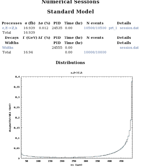
11.2 with only diagram
In this example, we will evaluate the process
and remove the
diagrams that do not correspond to . Our batch file
can be found at $CALCHEP/utile/batch_file_2
and has the following form:
Model:         Standard Model
Model changed: False
Gauge:         Feynman
Process:       e,E->m,M,h
Decay:         h-> b,B
Remove:        A,e,m

pdf1:      ISR & Beamstrahlung
pdf2:      ISR & Beamstrahlung
Bunch x+y sizes (nm)Ψ  : 560
Bunch length (mm)Ψ  : 0.4
Number of particlesΨ  : 2E+10

p1:        500
p2:        500

Parameter: Mh=125

Regularization momentum: 34
Regularization mass:     MZ
Regularization width:    wZ
Regularization power:    2

Dist parameter:    M(m,M)
Dist min:Ψ   0
Dist max:Ψ   120
Dist n bins:Ψ   100
Dist title:Ψ   e,E->m,M,h
Dist x-title:Ψ   M(m,M) (GeV)

Number of events (per run step): 10000
Filename:                        ee_mmh_mmbb

nSess_1:   5
nCalls_1:  100000
nSess_2:   5
nCalls_2:  100000
One should note three new elements
in this batch as compared to the previous one:
1. Decay: this statement generates Higgs boson decay
which is automatically connected to the production mode;
2. Remove: this statement specifies that diagrams with internal
photons, electrons or muons should be removed (that is, only the
process is kept).
3. Regularization: this statement is used to perform a more efficient integration of the
Z-boson resonance peak.
By running
./calchep_batch batch_file_2
the batch interface will calculate the cross section,
generate 10K events with a final state
written in the ee_mmh_mmbb-single.lhe file.
The total cross section of this process is 0.517 fb.
Again, the user can check the results in his/her web browser which
should agree with
Fig. 5.
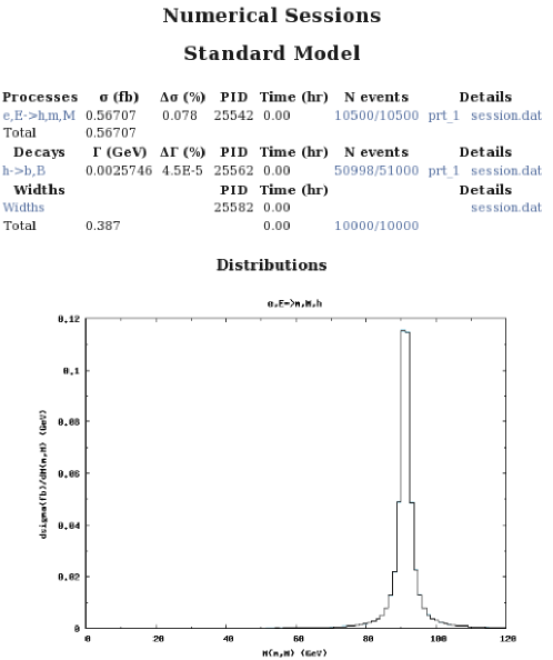
11.3
In this example, we consider the process
.
The batch file can be found at $CALCHEP/utile/batch_file_3
and has the following form:
Model:         Standard Model(CKM=1)
Model changed: False
Gauge:         Feynman

Process:   p,p->W,b,B
Decay:     W->le,n
Composite: p=u,U,d,D,s,S,c,C,b,B,G
Composite: W=W+,W-
Composite: le=e,E,m,M
Composite: n=ne,Ne,nm,Nm
Composite: jet=u,U,d,D,s,S,c,C,b,B,G

pdf1:      cteq6l (proton)
pdf2:      cteq6l (proton)
p1:        4000
p2:        4000

Run parameter: Mh
Run begin:     120
Run step size: 5
Run n steps:   3

alpha Q :            M45

Cut parameter:    M(b,B)
Cut invert:       False
Cut min:          100
Cut max:

Cut parameter:    J(jet,jet)
Cut invert:       False
Cut min:          0.5
Cut max:

Cut parameter:    T(jet)
Cut invert:       False
Cut min:          20
Cut max:

Kinematics :      12 -> 3, 45
Kinematics :      45 -> 4 , 5

Regularization momentum: 45
Regularization mass:     Mh
Regularization width:    wh
Regularization power:    2


Dist parameter:    M(b,B)
Dist min:          100
Dist max:          200
Dist n bins:       100
Dist title:        p,p->W,b,B
Dist x-title:      M(b,B) (GeV)

Dist parameter:    M(W,jet)
Dist min:Ψ   100
Dist max:Ψ   200
Dist n bins:Ψ   100
Dist title:Ψ   p,p->W,b,B
Dist x-title:Ψ   M(W,jet) (GeV)

Number of events (per run step): 10000
Filename:                        pp_Wbb_enbb

nSess_1:   5
nCalls_1:  100000
nSess_2:   5
nCalls_2:  100000
A new feature of this batch file is that it performs a scan of
as a function of the Higgs boson mass
using the Run parameter statement.
The result of this scan can be seen on a web browser as shown in Fig. 6.
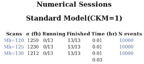
Further details on the individual numerical sessions can be checked by clicking
on a
particular value of the running parameter. For example, clicking on
Mh=120 in the web browser will lead to the html page shown in
Fig.7.
This page also presents the requested distributions.
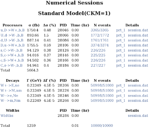
We would like to note that all
the results shown in the html browser are also recorded in the pure text files
located in the $WORK/html directory.
For example, the results for the numerical session are recorded in the file
$WORK/html/numerical.txt as well as in the files in the $WORK/html/runs
directory which contain further details.
For example, after a successful run of the file batch_file_3 given in the example above,
the user should get the file
$WORK/html/numerical.txt with the following lines:
ΨCalcHEP Numerical Details

ΨDone!

Scans               sigma (fb)     Running   Finished   Time (hr)   N events
Mh120               1.2610e+03       0/13     13/13     0.01        10000
Mh125               1.2510e+03       0/13     13/13     0.01        10000
Mh130               1.2440e+03       0/13     13/13     0.01        10000
12 Conclusions and outlook
The new version of CalcHEP, version 3.4 presented here is ready
to explore the Standard Model and BSM models by theorists, phenomenologists and experimentalists.
CalcHEP can be used:
1) via an interactive GUI interface which allows to understand the anatomy of the process under
study including details of the interference;
2) via a batch interface which highly automatizes and parallelizes the evaluation
of numerous production and decay processes as well as conencting them together at the stage of event generaton;
3) through the High Energy Physics Model Database (HEPMDB) using the resources
of a powerful HPC cluster
which allowes to perform an exaustive scan of the model parameter space
and generate numerous LHE files in one run.
We should also stress that there are many BSM models available for CalcHEPat the HEPMDB site and it is easy to implement new models by means of the LanHEP and FeynRules packages.
The next development of CalcHEP will include
1) an implementation of an automatic regularisation procedure.
2) an implemention of projections on polarization
states of the massive fermions and vector bosons
3) taking into account spin correlatons
for the processes when connecting production and decays.
4) an implementation of the jet matching procedure which will allow to properly combine
subprocess with multi-jet final states.
5) an implementation of the helicity amplitude method which allows to evaluate
processes with larger final state particles multiplicity as well as
spin correlation when connecting production and decay processes.
6) a new improved interactive numerical session which sums over the
subprocesses and connects production and decay processes in the GUI as
well as parallelizing over multiple cpus on a multicore machine.
Work in all these directions is in progress.
The CalcHEP team is open to additional sugegstions/requests from users.
Acknowledgements
AB would like to thank the NExT Institute and SEPnet for partial financial support. The work of AB and AP was strongly supported by the Royal Society grant JP090598. AP was also supported by the Russian foundation for Basic Research, grants 10-02-01443-a and 12-02-93108-CNRSL−a. The work of NC was supported in part by the US National Science Foundation under grant PHY-0354226, the LHC-TI initiative of the US National Science Foundation under grant PHY-0705682, the PITTsburgh Particle physics, Astrophysics, and Cosmology Center, and the US Department of Energy under grant DE- FG02-12ER41832.
A large part of the recent developments in CalcHEP were motivated by requests for the micrOMEGAs package which uses CalcHEP as a generator of matrix elements. We thank Genevieve Belanger and Fawzi Boudjema for helpful comments and suggestions in the development of CalcHEP.
CalcHEP is also know for its succesful usage of various SM extensions mainly due to the pioneering work of Andrey Semenov in the development of the LanHEP package which allows to realize rather complicated models in CalcHEP notation. We are grateful to Andrey Semenov for this job.
NC would like to thank Fabio Maltoni and Claude Duhr for their support in writing a CalcHEP output for the FeynRules package.
In 2009 AB and AP worked together at the Galileo Galilei Institute for Theoretical Physics where part of the CalcHEP development was performed. We are grateful to GGI for this opportunity.
We are especially thankful to Maksym Bondarenko, the main author of the HEPMDB project which has turned out to be very important for various web applications of CalcHEP.
We are grateful for many people who have tested CalcHEP, especially to Lorenzo Basso, Alexandra Carvalho, Joydeep Chakrabortty, Qing-Hong Cao, Mikhail Chizhov, Asesh Datta, Mads Frandsen, Renato Guedes, K.C. Kong, Tomas Lastovicka, Orlando Panella, Rui Santos, Chloe Papineau, Marco Pruna, Patrik Svantesson, Florian Staub, Daniel Stolarski, Riccardo Torre, Izmail Turan and Alfonso Zerwekh.
References
- [1] A. Pukhov, et al., CompHEP: A package for evaluation of Feynman diagrams and integration over multi-particle phase space. User’s manual for version 33 (1999). arXiv:hep-ph/9908288.
- [2] H. Tanaka, T. Kaneko, Y. Shimizu, Numerical calculation of Feynman amplitudes for electroweak theories and an application to e+ e- W+ W- gamma, Comput. Phys. Commun. 64 (1991) 149–166. doi:10.1016/0010-4655(91)90058-S.
- [3] F. Yuasa, et al., Automatic computation of cross sections in HEP: Status of GRACE system, Prog. Theor. Phys. Suppl. 138 (2000) 18–23. arXiv:hep-ph/0007053.
- [4] G. Belanger, et al., Automatic calculations in high energy physics and Grace at one-loop, Phys. Rept. 430 (2006) 117–209. arXiv:hep-ph/0308080, doi:10.1016/j.physrep.2006.02.001.
- [5] H. Murayama, I. Watanabe, K. Hagiwara, HELAS: HELicity amplitude subroutines for Feynman diagram evaluationsKEK-91-11.
- [6] E. Boos, et al., CompHEP 4.4: Automatic computations from Lagrangians to events, Nucl. Instrum. Meth. A534 (2004) 250–259. arXiv:hep-ph/0403113, doi:10.1016/j.nima.2004.07.096.
- [7] J. Kublbeck, M. Bohm, A. Denner, FEYN ARTS: COMPUTER ALGEBRAIC GENERATION OF FEYNMAN GRAPHS AND AMPLITUDES, Comput. Phys. Commun. 60 (1990) 165–180. doi:10.1016/0010-4655(90)90001-H.
- [8] T. Hahn, Generating Feynman diagrams and amplitudes with FeynArts 3, Comput. Phys. Commun. 140 (2001) 418–431. arXiv:hep-ph/0012260, doi:10.1016/S0010-4655(01)00290-9.
- [9] T. Hahn, Automatic loop calculations with FeynArts, FormCalc, and LoopTools, Nucl. Phys. Proc. Suppl. 89 (2000) 231–236. arXiv:hep-ph/0005029, doi:10.1016/S0920-5632(00)00848-3.
- [10] F. Maltoni, T. Stelzer, MadEvent: Automatic event generation with MadGraph, JHEP 02 (2003) 027. arXiv:hep-ph/0208156.
- [11] J. Alwall, M. Herquet, F. Maltoni, O. Mattelaer, T. Stelzer, MadGraph 5 : Going Beyond, JHEP 06 (2011) 128. arXiv:1106.0522, doi:10.1007/JHEP06(2011)128.
- [12] A. Kanaki, C. G. Papadopoulos, HELAC: A package to compute electroweak helicity amplitudes, Comput. Phys. Commun. 132 (2000) 306–315. arXiv:hep-ph/0002082, doi:10.1016/S0010-4655(00)00151-X.
- [13] C. G. Papadopoulos, PHEGAS: A phase space generator for automatic cross- section computation, Comput. Phys. Commun. 137 (2001) 247–254. arXiv:hep-ph/0007335, doi:10.1016/S0010-4655(01)00163-1.
- [14] A. Cafarella, C. G. Papadopoulos, M. Worek, Helac-Phegas: a generator for all parton level processes, Comput. Phys. Commun. 180 (2009) 1941–1955. arXiv:0710.2427, doi:10.1016/j.cpc.2009.04.023.
- [15] M. Moretti, T. Ohl, J. Reuter, O’Mega: An optimizing matrix element generatorarXiv:hep-ph/0102195.
- [16] W. Kilian, T. Ohl, J. Reuter, WHIZARD: Simulating Multi-Particle Processes at LHC and ILC (2007). arXiv:0708.4233.
- [17] T. Gleisberg, et al., SHERPA 1.alpha, a proof-of-concept version, JHEP 02 (2004) 056. arXiv:hep-ph/0311263, doi:10.1088/1126-6708/2004/02/056.
- [18] T. Gleisberg, et al., Event generation with SHERPA 1.1, JHEP 02 (2009) 007. arXiv:0811.4622, doi:10.1088/1126-6708/2009/02/007.
- [19] A. Pukhov, CalcHEP 2.3: MSSM, structure functions, event generation, batchs, and generation of matrix elements for other packages (2004). arXiv:hep-ph/0412191.
- [20] A. Belyaev, A. Gladyshev, A. Semenov, Minimal supersymmetric standard model within compHEP software packagearXiv:hep-ph/9712303.
- [21] G. Belanger, F. Boudjema, A. Pukhov, A. Semenov, micromegas: A program for calculating the relic density in the mssm, Comput. Phys. Commun. 149 (2002) 103–120. arXiv:hep-ph/0112278.
- [22] G. Belanger, F. Boudjema, C. Hugonie, A. Pukhov, A. Semenov, Relic density of dark matter in the NMSSM, JCAP 0509 (2005) 001. arXiv:hep-ph/0505142, doi:10.1088/1475-7516/2005/09/001.
- [23] G. Belanger, F. Boudjema, S. Kraml, A. Pukhov, A. Semenov, Relic density of neutralino dark matter in the MSSM with CP violation, Phys. Rev. D73 (2006) 115007. arXiv:hep-ph/0604150, doi:10.1103/PhysRevD.73.115007.
- [24] A. Belyaev, C. Leroy, R. Mehdiyev, A. Pukhov, Leptoquark single and pair production at LHC with CalcHEP/CompHEP in the complete model, JHEP 09 (2005) 005. arXiv:hep-ph/0502067.
- [25] A. Belyaev, C.-R. Chen, K. Tobe, C. Yuan, Phenomenology of littlest Higgs model with T-parity: Including effects of T-odd fermions (2006) 1113–1116.
- [26] A. Belyaev, et al., Technicolor Walks at the LHC, Phys. Rev. D79 (2009) 035006. arXiv:0809.0793, doi:10.1103/PhysRevD.79.035006.
- [27] G. Belanger, M. Kakizaki, A. Pukhov, Dark matter in UED: The Role of the second KK level, JCAP 1102 (2011) 009. arXiv:1012.2577, doi:10.1088/1475-7516/2011/02/009.
- [28] G. Brooijmans, B. Gripaios, F. Moortgat, J. Santiago, P. Skands, et al., Les Houches 2011: Physics at TeV Colliders New Physics Working Group ReportarXiv:1203.1488.
- [29] B. C. Allanach, Softsusy: A c++ program for calculating supersymmetric spectra, Comput. Phys. Commun. 143 (2002) 305–331. arXiv:hep-ph/0104145.
- [30] W. Porod, Spheno, a program for calculating supersymmetric spectra, susy particle decays and susy particle production at e+ e- colliders, Comput. Phys. Commun. 153 (2003) 275–315. arXiv:hep-ph/0301101.
- [31] U. Ellwanger, C. Hugonie, NMSPEC: A Fortran code for the sparticle and Higgs masses in the NMSSM with GUT scale boundary conditions, Comput. Phys. Commun. 177 (2007) 399–407. arXiv:hep-ph/0612134, doi:10.1016/j.cpc.2007.05.001.
- [32] J. Lee, A. Pilaftsis, M. S. Carena, S. Choi, M. Drees, et al., CPsuperH: A Computational tool for Higgs phenomenology in the minimal supersymmetric standard model with explicit CP violation, Comput.Phys.Commun. 156 (2004) 283–317. arXiv:hep-ph/0307377, doi:10.1016/S0010-4655(03)00463-6.
- [33] D. Chowdhury, R. Garani, S. K. Vempati, SUSEFLAV: Program for supersymmetric mass spectra with seesaw mechanism and rare lepton flavor violating decaysarXiv:1109.3551.
- [34] G. Belanger, N. D. Christensen, A. Pukhov, A. Semenov, SLHAplus: a library for implementing extensions of the standard model, Comput.Phys.Commun. 182 (2011) 763–774. arXiv:1008.0181, doi:10.1016/j.cpc.2010.10.025.
- [35] A. Semenov, LanHEP - a package for the automatic generation of Feynman rules in field theory. Version 3.0, Comput. Phys. Commun. 180 (2009) 431–454. arXiv:0805.0555, doi:10.1016/j.cpc.2008.10.012.
- [36] N. D. Christensen, C. Duhr, FeynRules - Feynman rules made easy, Comput. Phys. Commun. 180 (2009) 1614–1641. arXiv:0806.4194, doi:10.1016/j.cpc.2009.02.018.
- [37] F. Staub, SARAH, arXiv:0806.0538 [hep-ph]. arXiv:0806.0538.
- [38] G. Belanger, F. Boudjema, A. Pukhov, A. Semenov, micrOMEGAs2.0: A program to calculate the relic density of dark matter in a generic model, Comput. Phys. Commun. 176 (2007) 367–382. arXiv:hep-ph/0607059, doi:10.1016/j.cpc.2006.11.008.
- [39] G. Belanger, et al., Indirect search for dark matter with micrOMEGAs2.4, Comput. Phys. Commun. 182 (2011) 842–856. arXiv:1004.1092, doi:10.1016/j.cpc.2010.11.033.
- [40] K. Kong, TASI 2011: CalcHEP and PYTHIA TutorialsarXiv:1208.0035.
-
[41]
Pardicle data group.
URL http://pdg.lbl.gov - [42] T. Sjostrand, High-energy physics event generation with PYTHIA 5.7 and JETSET 7.4, Comput. Phys. Commun. 82 (1994) 74–90. doi:10.1016/0010-4655(94)90132-5.
- [43] P. Z. Skands, et al., SUSY Les Houches Accord: Interfacing SUSY Spectrum Calculators, Decay Packages, and Event Generators, JHEP 07 (2004) 036. arXiv:hep-ph/0311123, doi:10.1088/1126-6708/2004/07/036.
- [44] B. C. Allanach, et al., SUSY Les Houches Accord 2, Comp. Phys. Commun. 180 (2009) 8–25. arXiv:0801.0045, doi:10.1016/j.cpc.2008.08.004.
- [45] M. R. Whalley, D. Bourilkov, R. C. Group, The Les Houches Accord PDFs (LHAPDF) and LhagluearXiv:hep-ph/0508110.
- [46] G. P. Lepage, A New Algorithm for Adaptive Multidimensional Integration, J. Comput. Phys. 27 (1978) 192. doi:10.1016/0021-9991(78)90004-9.
- [47] W. Press, S. Teukolsky, W. Vetterling, B. Flannery, Numerical recipes in C: the art of scientific computing, Cambridge University Press, 1999.
- [48] J. Alwall, et al., A standard format for Les Houches event files, Comput. Phys. Commun. 176 (2007) 300–304. arXiv:hep-ph/0609017, doi:10.1016/j.cpc.2006.11.010.
- [49] S. Belov, L. Dudko, D. Kekelidze, A. Sherstnev, HepML, an XML-based format for describing simulated data in high energy physics, Comput. Phys. Commun. 181 (2010) 1758–1768. arXiv:1001.2576, doi:10.1016/j.cpc.2010.06.026.
- [50] A. Pukhov, Batch calculations in CalcHEP, Nucl.Instrum.Meth. A502 (2003) 573–575.
- [51] J. Alwall, P. Demin, S. de Visscher, R. Frederix, M. Herquet, et al., MadGraph/MadEvent v4: The New Web Generation, JHEP 0709 (2007) 028. arXiv:0706.2334, doi:10.1088/1126-6708/2007/09/028.
- [52] J. Bjorken, S. Drell, Relativistic quantum mechanics, International series in pure and applied physics, McGraw-Hill, 1964.
-
[53]
F. E. Paige, S. D. Protopopescu, H. Baer, X. Tata,
ISAJET 7.69: A Monte Carlo event
generator for pp, anti-p p, and e+e- reactionsarXiv:hep-ph/0312045.
URL http://www.nhn.ou.edu/~isajet/ - [54] A. Djouadi, J.-L. Kneur, G. Moultaka, Suspect: A fortran code for the supersymmetric and higgs particle spectrum in the mssm, hep-ph/0211331 (2002).
- [55] A. Djouadi, The Anatomy of electro-weak symmetry breaking. I: The Higgs boson in the standard model, Phys.Rept. 457 (2008) 1–216. arXiv:hep-ph/0503172, doi:10.1016/j.physrep.2007.10.004.
- [56] A. Djouadi, The Anatomy of electro-weak symmetry breaking. II. The Higgs bosons in the minimal supersymmetric model, Phys.Rept. 459 (2008) 1–241. arXiv:hep-ph/0503173, doi:10.1016/j.physrep.2007.10.005.
- [57] K. Chetyrkin, B. A. Kniehl, M. Steinhauser, Hadronic Higgs decay to order alpha-s**4, Phys.Rev.Lett. 79 (1997) 353–356. arXiv:hep-ph/9705240, doi:10.1103/PhysRevLett.79.353.
- [58] K. Chetyrkin, B. A. Kniehl, M. Steinhauser, W. A. Bardeen, Effective QCD interactions of CP odd Higgs bosons at three loops, Nucl.Phys. B535 (1998) 3–18. arXiv:hep-ph/9807241.
- [59] M. Spira, A. Djouadi, D. Graudenz, P. Zerwas, Higgs boson production at the LHC, Nucl.Phys. B453 (1995) 17–82. arXiv:hep-ph/9504378, doi:10.1016/0550-3213(95)00379-7.
- [60] P. Baikov, K. Chetyrkin, Higgs Decay into Hadrons to Order alpha**5(s), Phys.Rev.Lett. 97 (2006) 061803. arXiv:hep-ph/0604194, doi:10.1103/PhysRevLett.97.061803.
- [61] S. Dawson, A. Djouadi, M. Spira, Qcd corrections to susy higgs production: The role of squark loops, Phys. Rev. Lett. 77 (1996) 16–19. arXiv:hep-ph/9603423.
- [62] S. Dittmaier, S. Dittmaier, C. Mariotti, G. Passarino, R. Tanaka, et al., Handbook of LHC Higgs Cross Sections: 2. Differential DistributionsarXiv:1201.3084.
- [63] R. Barbieri, L. J. Hall, V. S. Rychkov, Improved naturalness with a heavy Higgs: An Alternative road to LHC physics, Phys.Rev. D74 (2006) 015007. arXiv:hep-ph/0603188, doi:10.1103/PhysRevD.74.015007.
- [64] L. Lopez Honorez, C. E. Yaguna, The inert doublet model of dark matter revisited, JHEP 09 (2010) 046. arXiv:1003.3125, doi:10.1007/JHEP09(2010)046.
- [65] J. Kublbeck, H. Eck, R. Mertig, Computeralgebraic generation and calculation of Feynman graphs using FeynArts and FeynCalc, Nucl. Phys. Proc. Suppl. 29A (1992) 204–208.
- [66] P. de Aquino, W. Link, F. Maltoni, O. Mattelaer, T. Stelzer, ALOHA: Automatic Libraries Of Helicity Amplitudes for Feynman Diagram Computations, Comput.Phys.Commun. 183 (2012) 2254–2263. arXiv:1108.2041, doi:10.1016/j.cpc.2012.05.004.
- [67] C. Degrande, C. Duhr, B. Fuks, D. Grellscheid, O. Mattelaer, et al., UFO - The Universal FeynRules Output, Comput.Phys.Commun. 183 (2012) 1201–1214. arXiv:1108.2040, doi:10.1016/j.cpc.2012.01.022.