Determinantal point processes for machine learning
Abstract
Determinantal point processes (DPPs) are elegant probabilistic models of repulsion that arise in quantum physics and random matrix theory. In contrast to traditional structured models like Markov random fields, which become intractable and hard to approximate in the presence of negative correlations, DPPs offer efficient and exact algorithms for sampling, marginalization, conditioning, and other inference tasks. We provide a gentle introduction to DPPs, focusing on the intuitions, algorithms, and extensions that are most relevant to the machine learning community, and show how DPPs can be applied to real-world applications like finding diverse sets of high-quality search results, building informative summaries by selecting diverse sentences from documents, modeling non-overlapping human poses in images or video, and automatically building timelines of important news stories.
1 Introduction
Probabilistic modeling and learning techniques have become indispensable tools for analyzing data, discovering patterns, and making predictions in a variety of real-world settings. In recent years, the widespread availability of both data and processing capacity has led to new applications and methods involving more complex, structured output spaces, where the goal is to simultaneously make a large number of interrelated decisions. Unfortunately, the introduction of structure typically involves a combinatorial explosion of output possibilities, making inference computationally impractical without further assumptions.
A popular compromise is to employ graphical models, which are tractable when the graph encoding local interactions between variables is a tree. For loopy graphs, inference can often be approximated in the special case when the interactions between variables are positive and neighboring nodes tend to have the same labels. However, dealing with global, negative interactions in graphical models remains intractable, and heuristic methods often fail in practice.
Determinantal point processes (DPPs) offer a promising and complementary approach. Arising in quantum physics and random matrix theory, DPPs are elegant probabilistic models of global, negative correlations, and offer efficient algorithms for sampling, marginalization, conditioning, and other inference tasks. While they have been studied extensively by mathematicians, giving rise to a deep and beautiful theory, DPPs are relatively new in machine learning. We aim to provide a comprehensible introduction to DPPs, focusing on the intuitions, algorithms, and extensions that are most relevant to our community.
1.1 Diversity
A DPP is a distribution over subsets of a fixed ground set, for instance, sets of search results selected from a large database. Equivalently, a DPP over a ground set of items can be seen as modeling a binary characteristic vector of length . The essential characteristic of a DPP is that these binary variables are negatively correlated; that is, the inclusion of one item makes the inclusion of other items less likely. The strengths of these negative correlations are derived from a kernel matrix that defines a global measure of similarity between pairs of items, so that more similar items are less likely to co-occur. As a result, DPPs assign higher probability to sets of items that are diverse; for example, a DPP will prefer search results that cover multiple distinct aspects of a user’s query, rather than focusing on the most popular or salient one.
This focus on diversity places DPPs alongside a number of recently developed techniques for working with diverse sets, particularly in the information retrieval community (Carbonell and Goldstein, 1998; Zhai et al., 2003; Chen and Karger, 2006; Yue and Joachims, 2008; Radlinski et al., 2008; Swaminathan et al., 2009; Raman et al., 2012). However, unlike these methods, DPPs are fully probabilistic, opening the door to a wider variety of potential applications, without compromising algorithmic tractability.
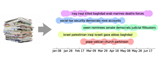
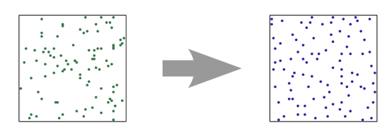
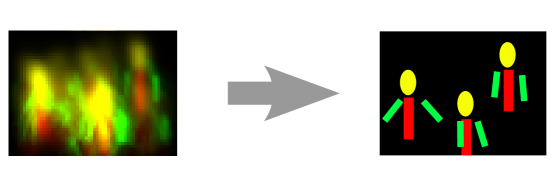
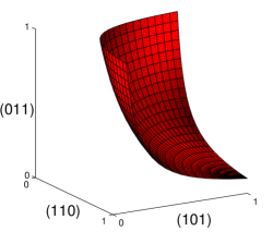
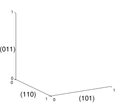
The general concept of diversity can take on a number of forms depending on context and application. Including multiple kinds of search results might be seen as covering or summarizing relevant interpretations of the query or its associated topics; see Figure 1. Alternatively, items inhabiting a continuous space may exhibit diversity as a result of repulsion, as in Figure 2. In fact, certain repulsive quantum particles are known to be precisely described by a DPP; however, a DPP can also serve as a model for general repulsive phenomena, such as the locations of trees in a forest, which appear diverse due to physical and resource constraints. Finally, diversity can be used as a filtering prior when multiple selections must be based on a single detector or scoring metric. For instance, in Figure 3 a weak pose detector favors large clusters of poses that are nearly identical, but filtering through a DPP ensures that the final predictions are well-separated.
Throughout this survey we demonstrate applications for DPPs in a variety of settings, including:
-
•
The DUC 2003/2004 text summarization task, where we form extractive summaries of news articles by choosing diverse subsets of sentences (Section 4.2.1);
-
•
An image search task, where we model human judgments of diversity for image sets returned by Google Image Search (Section 5.3);
-
•
A multiple pose estimation task, where we improve the detection of human poses in images from television shows by incorporating a bias toward non-overlapping predictions (Section 6.4);
-
•
A news threading task, where we automatically extract timelines of important news stories from a large corpus by balancing intra-timeline coherence with inter-timeline diversity (Section 6.6.4).
1.2 Outline
In this paper we present general mathematical background on DPPs along with a range of modeling extensions, efficient algorithms, and theoretical results that aim to enable practical modeling and learning. The material is organized as follows.
Section 2: Determinantal point processes.
We begin with an introduction to determinantal point processes tailored to the interests of the machine learning community. We focus on discrete DPPs, emphasizing intuitions and including new, simplified proofs for some theoretical results. We provide descriptions of known efficient inference algorithms, and characterize their computational properties.
Section 3: Representation and algorithms.
We describe a decomposition of the DPP that makes explicit its fundamental tradeoff between quality and diversity. We compare the expressive power of DPPs and MRFs, characterizing the tradeoffs in terms of modeling power and computational efficiency. We also introduce a dual representation for DPPs, showing how it can be used to perform efficient inference over large ground sets. When the data are high-dimensional and dual inference is still too slow, we show that random projections can be used to maintain a provably close approximation to the original model while greatly reducing computational requirements.
Section 4: Learning.
We derive an efficient algorithm for learning the parameters of a quality model when the diversity model is held fixed. We employ this learning algorithm to perform extractive summarization of news text.
Section 5: -DPPs.
We present an extension of DPPs that allows for explicit control over the number of items selected by the model. We show not only that this extension solves an important practical problem, but also that it increases expressive power: a -DPP can capture distributions that a standard DPP cannot. The extension to -DPPs necessitates new algorithms for efficient inference based on recursions for the elementary symmetric polynomials. We validate the new model experimentally on an image search task.
Section 6: Structured DPPs.
We extend DPPs to model diverse sets of structured items, such as sequences or trees, where there are combinatorially many possible configurations. In this setting the number of possible subsets is doubly-exponential, presenting a daunting computational challenge. However, we show that a factorization of the quality and diversity models together with the dual representation for DPPs makes efficient inference possible using second-order message passing. We demonstrate structured DPPs on a toy geographical paths problem, a still-image multiple pose estimation task, and two high-dimensional text threading tasks.
2 Determinantal point processes
Determinantal point processes (DPPs) were first identified as a class by Macchi (1975), who called them “fermion processes” because they give the distributions of fermion systems at thermal equilibrium. The Pauli exclusion principle states that no two fermions can occupy the same quantum state; as a consequence fermions exhibit what is known as the “anti-bunching” effect. This repulsion is described precisely by a DPP.
In fact, years before Macchi gave them a general treatment, specific DPPs appeared in major results in random matrix theory (Mehta and Gaudin, 1960; Dyson, 1962a, b, c; Ginibre, 1965), where they continue to play an important role (Diaconis, 2003; Johansson, 2005b). Recently, DPPs have attracted a flurry of attention in the mathematics community (Borodin and Olshanski, 2000; Borodin and Soshnikov, 2003; Borodin and Rains, 2005; Borodin et al., 2010; Burton and Pemantle, 1993; Johansson, 2002, 2004, 2005a; Okounkov, 2001; Okounkov and Reshetikhin, 2003; Shirai and Takahashi, 2000), and much progress has been made in understanding their formal combinatorial and probabilistic properties. The term “determinantal” was first used by Borodin and Olshanski (2000), and has since become accepted as standard. Many good mathematical surveys are now available (Borodin, 2009; Hough et al., 2006; Shirai and Takahashi, 2003a, b; Lyons, 2003; Soshnikov, 2000; Tao, 2009).
We begin with an overview of the aspects of DPPs most relevant to the machine learning community, emphasizing intuitions, algorithms, and computational properties.
2.1 Definition
A point process on a ground set is a probability measure over “point patterns” or “point configurations” of , which are finite subsets of . For instance, could be a continuous time interval during which a scientist records the output of a brain electrode, with characterizing the likelihood of seeing neural spikes at times , , and . Depending on the experiment, the spikes might tend to cluster together, or they might occur independently, or they might tend to spread out in time. captures these correlations.
For the remainder of this paper, we will focus on discrete, finite point processes, where we assume without loss of generality that ; in this setting we sometimes refer to elements of as items. Much of our discussion extends to the continuous case, but the discrete setting is computationally simpler and often more appropriate for real-world data—e.g., in practice, the electrode voltage will only be sampled at discrete intervals. The distinction will become even more apparent when we apply our methods to with no natural continuous interpretation, such as the set of documents in a corpus.
In the discrete case, a point process is simply a probability measure on , the set of all subsets of . A sample from might be the empty set, the entirety of , or anything in between. is called a determinantal point process if, when is a random subset drawn according to , we have, for every ,
| (1) |
for some real, symmetric matrix indexed by the elements of .111In general, need not be symmetric. However, in the interest of simplicity, we proceed with this assumption; it is not a significant limitation for our purposes. Here, denotes the restriction of to the entries indexed by elements of , and we adopt . Note that normalization is unnecessary here, since we are defining marginal probabilities that need not sum to 1.
Since is a probability measure, all principal minors of must be nonnegative, and thus itself must be positive semidefinite. It is possible to show in the same way that the eigenvalues of are bounded above by one using Equation (35), which we introduce later. These requirements turn out to be sufficient: any , , defines a DPP. This will be a consequence of Theorem 2.3.
We refer to as the marginal kernel since it contains all the information needed to compute the probability of any subset being included in . A few simple observations follow from Equation (1). If is a singleton, then we have
| (2) |
That is, the diagonal of gives the marginal probabilities of inclusion for individual elements of . Diagonal entries close to 1 correspond to elements of that are almost always selected by the DPP. Furthermore, if is a two-element set, then
| (5) | ||||
| (6) | ||||
| (7) |
Thus, the off-diagonal elements determine the negative correlations between pairs of elements: large values of imply that and tend not to co-occur.
Equation (7) demonstrates why DPPs are “diversifying”. If we think of the entries of the marginal kernel as measurements of similarity between pairs of elements in , then highly similar elements are unlikely to appear together. If , then and are “perfectly similar” and do not appear together almost surely. Conversely, when is diagonal there are no correlations and the elements appear independently. Note that DPPs cannot represent distributions where elements are more likely to co-occur than if they were independent: correlations are always nonpositive.
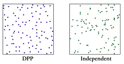
Figure 4 shows the difference between sampling a set of points in the plane using a DPP (with inversely related to the distance between points and ), which leads to a relatively uniformly spread set with good coverage, and sampling points independently, which results in random clumping.
2.1.1 Examples
In this paper, our focus is on using DPPs to model real-world data. However, many theoretical point processes turn out to be exactly determinantal, which is one of the main reasons they have received so much recent attention. In this section we briefly describe a few examples; some of them are quite remarkable on their own, and as a whole they offer some intuition about the types of distributions that are realizable by DPPs. Technical details for each example can be found in the accompanying reference.
Descents in random sequences (Borodin et al., 2010)
Given a sequence of random numbers drawn uniformly and independently from a finite set (say, the digits 0–9), the locations in the sequence where the current number is less than the previous number form a subset of . This subset is distributed as a determinantal point process. Intuitively, if the current number is less than the previous number, it is probably not too large, thus it becomes less likely that the next number will be smaller yet. In this sense, the positions of decreases repel one another.
Non-intersecting random walks (Johansson, 2004)
Consider a set of independent, simple, symmetric random walks of length on the integers. That is, each walk is a sequence where is either -1 or +1 with equal probability. If we let the walks begin at positions and condition on the fact that they end at positions and do not intersect, then the positions at any time are a subset of and distributed according to a DPP. Intuitively, if the random walks do not intersect, then at any time step they are likely to be far apart.
Edges in random spanning trees (Burton and Pemantle, 1993)
Let be an arbitrary finite graph with edges, and let be a random spanning tree chosen uniformly from the set of all the spanning trees of . The edges in form a subset of the edges of that is distributed as a DPP. The marginal kernel in this case is the transfer-impedance matrix, whose entry is the expected signed number of traversals of edge when a random walk begins at one endpoint of and ends at the other (the graph edges are first oriented arbitrarily). Thus, edges that are in some sense “nearby” in are similar according to , and as a result less likely to participate in a single uniformly chosen spanning tree. As this example demonstrates, some DPPs assign zero probability to sets whose cardinality is not equal to a particular ; in this case, is the number of nodes in the graph minus one—the number of edges in any spanning tree. We will return to this issue in Section 5.
Eigenvalues of random matrices (Ginibre, 1965; Mehta and Gaudin, 1960)
Let be a random matrix obtained by drawing every entry independently from the complex normal distribution. This is the complex Ginibre ensemble. The eigenvalues of , which form a finite subset of the complex plane, are distributed according to a DPP. If a Hermitian matrix is generated in the corresponding way, drawing each diagonal entry from the normal distribution and each pair of off-diagonal entries from the complex normal distribution, then we obtain the Gaussian unitary ensemble, and the eigenvalues are now a DPP-distributed subset of the real line.
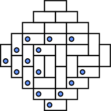
Aztec diamond tilings (Johansson, 2005a)
The Aztec diamond is a diamond-shaped union of lattice squares, as depicted in Figure 5a. (Half of the squares have been colored gray in a checkerboard pattern.) A domino tiling is a perfect cover of the Aztec diamond using rectangles, as in Figure 5b. Suppose that we draw a tiling uniformly at random from among all possible tilings. (The number of tilings is known to be exponential in the width of the diamond.) We can identify this tiling with the subset of the squares that are (a) painted gray in the checkerboard pattern and (b) covered by the left half of a horizontal tile or the bottom half of a vertical tile (see Figure 5c). This subset is distributed as a DPP.


2.2 L-ensembles
For the purposes of modeling real data, it is useful to slightly restrict the class of DPPs by focusing on L-ensembles. First introduced by Borodin and Rains (2005), an L-ensemble defines a DPP not through the marginal kernel , but through a real, symmetric matrix indexed by the elements of :
| (8) |
Whereas Equation (1) gave the marginal probabilities of inclusion for subsets , Equation (8) directly specifies the atomic probabilities for every possible instantiation of . As for , it is easy to see that must be positive semidefinite. However, since Equation (8) is only a statement of proportionality, the eigenvalues of need not be less than one; any positive semidefinite defines an L-ensemble. The required normalization constant can be given in closed form due to the fact that , where is the identity matrix. This is a special case of the following theorem.
Theorem 2.1.
For any ,
| (9) |
where is the diagonal matrix with ones in the diagonal positions corresponding to elements of , and zeros everywhere else.
Proof.
Suppose that ; then Equation (9) holds trivially. Now suppose inductively that the theorem holds whenever has cardinality less than . Given such that , let be an element of where . Splitting blockwise according to the partition , we can write
| (10) |
where is the subcolumn of the th column of whose rows correspond to , and similarly for . By multilinearity of the determinant, then,
| (15) | ||||
| (16) |
We can now apply the inductive hypothesis separately to each term, giving
| (17) | ||||
| (18) |
where we observe that every either contains and is included only in the first sum, or does not contain and is included only in the second sum. ∎
Thus we have
| (19) |
As a shorthand, we will write instead of when the meaning is clear.
We can write a version of Equation (7) for L-ensembles, showing that if is a measure of similarity then diversity is preferred:
| (20) |
In this case we are reasoning about the full contents of rather than its marginals, but the intuition is essentially the same. Furthermore, we have the following result of Macchi (1975).
Theorem 2.2.
An L-ensemble is a DPP, and its marginal kernel is
| (21) |
Proof.
Using Theorem 2.1, the marginal probability of a set is
| (22) | ||||
| (23) | ||||
| (24) |
We can use the fact that to simplify and obtain
| (25) | ||||
| (26) | ||||
| (27) |
where we let . Now, we observe that left multiplication by zeros out all the rows of a matrix except those corresponding to . Therefore we can split blockwise using the partition to get
| (30) | ||||
| (31) |
∎
Note that can be computed from an eigendecomposition of by a simple rescaling of eigenvalues:
| (32) |
Conversely, we can ask when a DPP with marginal kernel is also an L-ensemble. By inverting Equation (21), we have
| (33) |
and again the computation can be performed by eigendecomposition. However, while the inverse in Equation (21) always exists due to the positive coefficient on the identity matrix, the inverse in Equation (33) may not. In particular, when any eigenvalue of achieves the upper bound of 1, the DPP is not an L-ensemble. We will see later that the existence of the inverse in Equation (33) is equivalent to giving nonzero probability to the empty set. (This is somewhat analogous to the positive probability assumption in the Hammersley-Clifford theorem for Markov random fields.) This is not a major restriction, for two reasons. First, when modeling real data we must typically allocate some nonzero probability for rare or noisy events, so when cardinality is one of the aspects we wish to model, the condition is not unreasonable. Second, we will show in Section 5 how to control the cardinality of samples drawn from the DPP, thus sidestepping the representational limits of L-ensembles.
Modulo the restriction described above, and offer alternative representations of DPPs. Under both representations, subsets that have higher diversity, as measured by the corresponding kernel, have higher likelihood. However, while gives marginal probabilities, L-ensembles directly model the atomic probabilities of observing each subset of , which offers an appealing target for optimization. Furthermore, need only be positive semidefinite, while the eigenvalues of are bounded above. For these reasons we will focus our modeling efforts on DPPs represented as L-ensembles.
2.2.1 Geometry
Determinants have an intuitive geometric interpretation. Let be a x matrix such that . (Such a can always be found for when is positive semidefinite.) Denote the columns of by for . Then:
| (34) |
where the right hand side is the squared -dimensional volume of the parallelepiped spanned by the columns of corresponding to elements in .
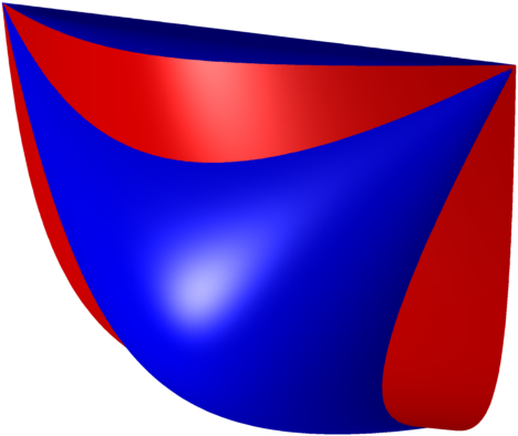
Intuitively, we can think of the columns of as feature vectors describing the elements of . Then the kernel measures similarity using dot products between feature vectors, and Equation (34) says that the probability assigned by a DPP to a set is related to the volume spanned by its associated feature vectors. This is illustrated in Figure 6.

From this intuition we can verify several important DPP properties. Diverse sets are more probable because their feature vectors are more orthogonal, and hence span larger volumes. Items with parallel feature vectors are selected together with probability zero, since their feature vectors define a degenerate parallelepiped. All else being equal, items with large-magnitude feature vectors are more likely to appear, because they multiply the spanned volumes for sets containing them.
We will revisit these intuitions in Section 3.1, where we decompose the kernel so as to separately model the direction and magnitude of the vectors .
2.3 Properties
In this section we review several useful properties of DPPs.
Restriction
If is distributed as a DPP with marginal kernel , then , where , is also distributed as a DPP, with marginal kernel .
Complement
If is distributed as a DPP with marginal kernel , then is also distributed as a DPP, with marginal kernel . In particular, we have
| (35) |
where indicates the identity matrix of appropriate size. It may seem counterintuitive that the complement of a diversifying process should also encourage diversity. However, it is easy to see that
| (36) | ||||
| (37) | ||||
| (38) | ||||
| (39) |
where the inequality follows from Equation (7).
Domination
If , that is, is positive semidefinite, then for all we have
| (40) |
In other words, the DPP defined by is larger than the one defined by in the sense that it assigns higher marginal probabilities to every set . An analogous result fails to hold for due to the normalization constant.
Scaling
If for some , then for all we have
| (41) |
It is easy to see that defines the distribution obtained by taking a random set distributed according to the DPP with marginal kernel , and then independently deleting each of its elements with probability .
Cardinality
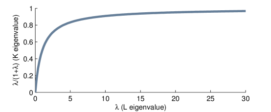
Let be the eigenvalues of . Then is distributed as the number of successes in Bernoulli trials, where trial succeeds with probability . This fact follows from Theorem 2.3, which we prove in the next section. One immediate consequence is that cannot be larger than . More generally, the expected cardinality of is
| (42) |
and the variance is
| (43) |
Note that, by Equation (21), are the eigenvalues of . Figure 7 shows a plot of the function . It is easy to see from this why the class of L-ensembles does not include DPPs where the empty set has probability zero—at least one of the Bernoulli trials would need to always succeed, and in turn one or more of the eigenvalues of would be infinite.
In some instances, the sum of Bernoullis may be an appropriate model for uncertain cardinality in real-world data, for instance when identifying objects in images where the number of objects is unknown in advance. In other situations, it may be more practical to fix the cardinality of up front, for instance when a set of exactly ten search results is desired, or to replace the sum of Bernoullis with an alternative cardinality model. We show how these goals can be can be achieved in Section 5.
2.4 Inference
One of the primary advantages of DPPs is that, although the number of possible realizations of is exponential in , many types of inference can be performed in polynomial time. In this section we review the inference questions that can (and cannot) be answered efficiently. We also discuss the empirical practicality of the associated computations and algorithms, estimating the largest values of that can be handled at interactive speeds (within 2–3 seconds) as well as under more generous time and memory constraints. The reference machine used for estimating real-world performance has eight Intel Xeon E5450 3Ghz cores and 32GB of memory.
2.4.1 Normalization
As we have already seen, the partition function, despite being a sum over terms, can be written in closed form as . Determinants of matrices can be computed through matrix decomposition in time, or reduced to matrix multiplication for better asymptotic performance. The Coppersmith-Winograd algorithm, for example, can be used to compute determinants in about time. Going forward, we will use to denote the exponent of whatever matrix multiplication algorithm is used.
Practically speaking, modern computers can calculate determinants up to at interactive speeds, or up to in about five minutes. When grows much larger, the memory required simply to store the matrix becomes limiting. (Sparse storage of larger matrices is possible, but computing determinants remains prohibitively expensive unless the level of sparsity is extreme.)
2.4.2 Marginalization
The marginal probability of any set of items can be computed using the marginal kernel as in Equation (1). From Equation (35) we can also compute the marginal probability that none of the elements in appear. (We will see below how marginal probabilities of arbitrary configurations can be computed using conditional DPPs.)
If the DPP is specified as an L-ensemble, then the computational bottleneck for marginalization is the computation of . The dominant operation is the matrix inversion, which requires at least time by reduction to multiplication, or using Gauss-Jordan elimination or various matrix decompositions, such as the eigendecomposition method proposed in Section 2.2. Since an eigendecomposition of the kernel will be central to sampling, the latter approach is often the most practical when working with DPPs.
Matrices up to can be inverted at interactive speeds, and problems up to can be completed in about ten minutes.
2.4.3 Conditioning
The distribution obtained by conditioning a DPP on the event that none of the elements in a set appear is easy to compute. For not intersecting with we have
| (44) | ||||
| (45) | ||||
| (46) |
where is the restriction of to the rows and columns indexed by elements in . In other words, the conditional distribution (over subsets of ) is itself a DPP, and its kernel is obtained by simply dropping the rows and columns of that correspond to elements in .
We can also condition a DPP on the event that all of the elements in a set are observed. For not intersecting with we have
| (47) | ||||
| (48) | ||||
| (49) |
where is the matrix with ones in the diagonal entries indexed by elements of and zeros everywhere else. Though it is not immediately obvious, Borodin and Rains (2005) showed that this conditional distribution (over subsets of ) is again a DPP, with a kernel given by
| (50) |
(Following the inversion, the matrix is restricted to rows and columns indexed by elements in , then inverted again.) It is easy to show that the inverses exist if and only if the probability of appearing is nonzero.
Combining Equation (46) and Equation (49), we can write the conditional DPP given an arbitrary combination of appearing and non-appearing elements:
| (51) |
The corresponding kernel is
| (52) |
Thus, the class of DPPs is closed under most natural conditioning operations.
General marginals
These formulas also allow us to compute arbitrary marginals. For example, applying Equation (21) to Equation (50) yields the marginal kernel for the conditional DPP given the appearance of :
| (53) |
Thus we have
| (54) |
(Note that is indexed by elements of , so this is only defined when and are disjoint.) Using Equation (35) for the complement of a DPP, we can now compute the marginal probability of any partial assignment, i.e.,
| (55) | ||||
| (56) |
Computing conditional DPP kernels in general is asymptotically as expensive as the dominant matrix inversion, although in some cases (conditioning only on non-appearance), the inversion is not necessary. In any case, conditioning is at most a small constant factor more expensive than marginalization.
2.4.4 Sampling
Algorithm 1, due to Hough et al. (2006), gives an efficient algorithm for sampling a configuration from a DPP. The input to the algorithm is an eigendecomposition of the DPP kernel . Note that is the th standard basis -vector, which is all zeros except for a one in the th position. We will prove the following theorem.
Theorem 2.3.
Let be an orthonormal eigendecomposition of a positive semidefinite matrix . Then Algorithm 1 samples .
Algorithm 1 has two main loops, corresponding to two phases of sampling. In the first phase, a subset of the eigenvectors is selected at random, where the probability of selecting each eigenvector depends on its associated eigenvalue. In the second phase, a sample is produced based on the selected vectors. Note that on each iteration of the second loop, the cardinality of increases by one and the dimension of is reduced by one. Since the initial dimension of is simply the number of selected eigenvectors (), Theorem 2.3 has the previously stated corollary that the cardinality of a random sample is distributed as a sum of Bernoulli variables.
To prove Theorem 2.3 we will first show that a DPP can be expressed as a mixture of simpler, elementary DPPs. We will then show that the first phase chooses an elementary DPP according to its mixing coefficient, while the second phase samples from the elementary DPP chosen in phase one.
Definition 2.4.
A DPP is called elementary if every eigenvalue of its marginal kernel is in . We write , where is a set of orthonormal vectors, to denote an elementary DPP with marginal kernel .
We introduce the term “elementary” here; Hough et al. (2006) refer to elementary DPPs as determinantal projection processes, since is an orthonormal projection matrix to the subspace spanned by . Note that, due to Equation (33), elementary DPPs are not generally L-ensembles. We start with a technical lemma.
Lemma 2.5.
Let for be an arbitrary sequence of rank-one matrices, and let denote the column of . Let . Then
| (57) |
Proof.
Expanding on the first column of using the multilinearity of the determinant,
| (58) |
and, applying the same operation inductively to all columns,
| (59) |
Since has rank one, the determinant of any matrix containing two or more columns of is zero; thus the terms in the sum vanish unless are distinct. ∎
Lemma 2.6.
A DPP with kernel is a mixture of elementary DPPs:
| (60) |
where denotes the set .
Proof.
Consider an arbitrary set , with . Let for ; note that all of the have rank one. From the definition of , the mixture distribution on the right hand side of Equation (60) gives the following expression for the marginal probability of :
| (61) |
Applying Lemma 57, this is equal to
| (62) | |||
| (63) | |||
| (64) | |||
| (65) |
using the fact that . Applying Lemma 57 in reverse and then the definition of in terms of the eigendecomposition of , we have that the marginal probability of given by the mixture is
| (66) |
Since the two distributions agree on all marginals, they are equal. ∎
Next, we show that elementary DPPs have fixed cardinality.
Lemma 2.7.
If is drawn according to an elementary DPP , then with probability one.
Proof.
Since has rank , whenever , so . But we also have
| (67) | ||||
| (68) | ||||
| (69) |
Thus almost surely. ∎
We can now prove the theorem.
Proof of Theorem 2.3.
Lemma 2.6 says that the mixture weight of is given by the product of the eigenvalues corresponding to the eigenvectors , normalized by . This shows that the first loop of Algorithm 1 selects an elementary DPP with probability equal to its mixture component. All that remains is to show that the second loop samples .
Let represent the matrix whose rows are the eigenvectors in , so that . Using the geometric interpretation of determinants introduced in Section 2.2.1, is equal to the squared volume of the parallelepiped spanned by . Note that since is an orthonormal set, is just the projection of onto the subspace spanned by .
Let . By Lemma 2.7 and symmetry, we can consider without loss of generality a single . Using the fact that any vector both in the span of and perpendicular to is also perpendicular to the projection of onto the span of , by the base height formula for the volume of a parallelepiped we have
| (70) |
where is the projection operator onto the subspace orthogonal to . Proceeding inductively,
| (71) |
Assume that, as iteration of the second loop in Algorithm 1 begins, we have already selected . Then in the algorithm has been updated to an orthonormal basis for the subspace of the original perpendicular to , and the probability of choosing is exactly
| (72) |
Therefore, the probability of selecting the sequence is
| (73) |
Since volume is symmetric, the argument holds identically for all of the orderings of . Thus the total probability that Algorithm 1 selects is . ∎
Corollary 2.8.
Algorithm 1 generates in uniformly random order.
Discussion
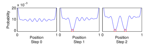
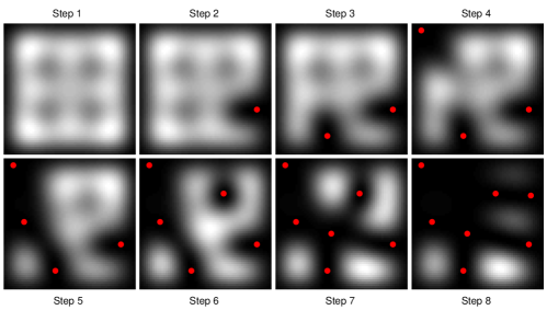
To get a feel for the sampling algorithm, it is useful to visualize the distributions used to select at each iteration, and to see how they are influenced by previously chosen items. Figure 8a shows this progression for a simple DPP where is a finely sampled grid of points in , and the kernel is such that points are more similar the closer together they are. Initially, the eigenvectors give rise to a fairly uniform distribution over points in , but as each successive point is selected and is updated, the distribution shifts to avoid points near those already chosen. Figure 8b shows a similar progression for a DPP over points in the unit square.
The sampling algorithm also offers an interesting analogy to clustering. If we think of the eigenvectors of as representing soft clusters, and the eigenvalues as representing their strengths—the way we do for the eigenvectors and eigenvalues of the Laplacian matrix in spectral clustering—then a DPP can be seen as performing a clustering of the elements in , selecting a random subset of clusters based on their strength, and then choosing one element per selected cluster. Of course, the elements are not chosen independently and cannot be identified with specific clusters; instead, the second loop of Algorithm 1 coordinates the choices in a particular way, accounting for overlap between the eigenvectors.
Algorithm 1 runs in time , where is the number of eigenvectors selected in phase one. The most expensive operation is the Gram-Schmidt orthonormalization required to compute . If is large, this can be reasonably expensive, but for most applications we do not want high-cardinality DPPs. (And if we want very high-cardinality DPPs, we can potentially save time by using Equation (35) to sample the complement instead.) In practice, the initial eigendecomposition of is often the computational bottleneck, requiring time. Modern multi-core machines can compute eigendecompositions up to at interactive speeds of a few seconds, or larger problems up to in around ten minutes. In some instances, it may be cheaper to compute only the top eigenvectors; since phase one tends to choose eigenvectors with large eigenvalues anyway, this can be a reasonable approximation when the kernel is expected to be low rank. Note that when multiple samples are desired, the eigendecomposition needs to be performed only once.
Deshpande and Rademacher (2010) recently proposed a -approximate algorithm for sampling that runs in time when is already decomposed as a Gram matrix, . When is known but an eigendecomposition is not (and is sufficiently large), this may be significantly faster than the exact algorithm.
2.4.5 Finding the mode
Finding the mode of a DPP—that is, finding the set that maximizes —is NP-hard. In conditional models, this problem is sometimes referred to as maximum a posteriori (or MAP) inference, and it is also NP-hard for most general structured models such as Markov random fields. Hardness was first shown for DPPs by Ko et al. (1995), who studied the closely-related maximum entropy sampling problem: the entropy of a set of jointly Gaussian random variables is given (up to constants) by the log-determinant of their covariance matrix; thus finding the maximum entropy subset of those variables requires finding the principal covariance submatrix with maximum determinant. Here, we adapt the argument of Çivril and Magdon-Ismail (2009), who studied the problem of finding maximum-volume submatrices.
Theorem 2.9.
Let dpp-mode be the optimization problem of finding, for a positive semidefinite input matrix indexed by elements of , the maximum value of over all . dpp-mode is NP-hard, and furthermore it is NP-hard even to approximate dpp-mode to a factor of .
Proof.
We reduce from exact 3-cover (X3C). An instance of X3C is a set and a collection of three-element subsets of ; the problem is to decide whether there is a sub-collection such that every element of appears exactly once in (that is, is an exact 3-cover). X3C is known to be NP-complete.
The reduction is as follows. Let , and let be an matrix where if contains and zero otherwise. Define , where . Note that the diagonal of is constant and equal to , and an off-diagonal entry is zero if and only if and do not intersect. is positive semidefinite by construction, and the reduction requires only polynomial time. Let . We will show that the maximum value of is greater than if and only if contains an exact 3-cover of .
If is an exact 3-cover of , then it must contain exactly 3-sets. Letting be the set of indices in , we have , and thus its determinant is .
Suppose there is no 3-cover of in . Let be an arbitrary subset of . If , then
| (74) |
Now suppose , and assume without loss of generality that . We have , and
| (75) |
By the base height formula,
| (76) |
Note that, since the columns of are normalized, each term in the product is at most one. Furthermore, at least of the terms must be strictly less than one, because otherwise there would be orthogonal columns, which would correspond to a 3-cover. By the construction of , if two columns and are not orthogonal then and overlap in at least one of three elements, so we have
| (77) | ||||
| (78) | ||||
| (79) |
Therefore,
| (80) | ||||
| (81) |
since .
We have shown that the existence of a 3-cover implies that the optimal value of dpp-mode is at least , while the optimal value cannot be more than if there is no 3-cover. Thus any algorithm that can approximate dpp-mode to better than a factor of can be used to solve X3C in polynomial time. We can choose to show that an approximation ratio of is NP-hard. ∎
Since there are only possible cardinalities for , Theorem 2.9 shows that dpp-mode is NP-hard even under cardinality constraints.
(Ko et al., 1995) propose an exact, exponential branch-and-bound algorithm for finding the mode using greedy heuristics to build candidate sets; they tested their algorithm on problems up to , successfully finding optimal solutions in up to about an hour. Modern computers are likely a few orders of magnitude faster; however, this algorithm is still probably impractical for applications with large . Çivril and Magdon-Ismail (2009) propose an efficient greedy algorithm for finding a set of size , and prove that it achieves an approximation ratio of . While this guarantee is relatively poor for all but very small , in practice the results may be useful nonetheless.
Submodularity
is log-submodular; that is,
| (82) |
whenever . Intuitively, adding elements to yields diminishing returns as gets larger. (This is easy to show by a volume argument.) Submodular functions can be minimized in polynomial time (Schrijver, 2000), and many results exist for approximately maximizing monotone submodular functions, which have the special property that supersets always have higher function values than their subsets (Nemhauser et al., 1978; Fisher et al., 1978; Feige, 1998). In Section 4.2.1 we will discuss how these kinds of greedy algorithms can be adapted for DPPs. However, in general is highly non-monotone, since the addition of even a single element can decrease the probability to zero.
Recently, Feige et al. (2007) showed that even non-monotone submodular functions can be approximately maximized in polynomial time using a local search algorithm, and a growing body of research has focused on extending this result in a variety of ways (Lee et al., 2009; Gharan and Vondrák, 2011; Vondrák et al., 2011; Feldman et al., 2011a, b; Chekuri et al., 2011). In our recent work we showed how the computational structure of DPPs gives rise to a particularly efficient variant of these methods (Kulesza et al., 2012).
2.5 Related processes
Historically, a wide variety of point process models have been proposed and applied to applications involving diverse subsets, particularly in settings where the items can be seen as points in a physical space and diversity is taken to mean some sort of “spreading” behavior. However, DPPs are essentially unique among this class in having efficient and exact algorithms for probabilistic inference, which is why they are particularly appealing models for machine learning applications. In this section we briefly survey the wider world of point processes and discuss the computational properties of alternative models; we will focus on point processes that lead to what is variously described as diversity, repulsion, (over)dispersion, regularity, order, and inhibition.
2.5.1 Poisson point processes
Perhaps the most fundamental point process is the Poisson point process, which is depicted on the right side of Figure 4 (Daley and Vere-Jones, 2003). While defined for continuous , in the discrete setting the Poisson point process can be simulated by flipping a coin independently for each item, and including those items for which the coin comes up heads. Formally,
| (83) |
where is the bias of the th coin. The process is called stationary when does not depend on ; in a spatial setting this means that no region has higher density than any other region.
A random set distributed as a Poisson point process has the property that whenever and are disjoint subsets of , the random variables and are independent; that is, the points in are not correlated. It is easy to see that DPPs generalize Poisson point processes by choosing the marginal kernel with and . This implies that inference for Poisson point processes is at least as efficient as for DPPs; in fact, it is more efficient, since for instance it is easy to compute the most likely configuration. However, since Poisson point processes do not model correlations between variables, they are rather uninteresting for most real-world applications.
Addressing this weakness, various procedural modifications of the Poisson process have been proposed in order to introduce correlations between items. While such constructions can be simple and intuitive, leading to straightforward sampling algorithms, they tend to make general statistical inference difficult.
Matérn repulsive processes
Matérn (1960, 1986) proposed a set of techniques for thinning Poisson point processes in order to induce a type of repulsion when the items are embedded in a Euclidean space. The Type I process is obtained from a Poisson set by removing all items in that lie within some radius of another item in . That is, if two items are close to each other, they are both removed; as a result all items in the final process are spaced at least a fixed distance apart. The Type II Matérn repulsive process, designed to achieve the same minimum distance property while keeping more items, begins by independently assigning each item in a uniformly random “time” in . Then, any item within a given radius of a point having a smaller time value is removed. Under this construction, when two items are close to each other only the later one is removed. Still, an item may be removed due to its proximity with an earlier item that was itself removed. This leads to the Type III process, which proceeds dynamically, eliminating items in time order whenever an earlier point which has not been removed lies within the radius.
Inference for the Matérn processes is computationally daunting. First and second order moments can be computed for Types I and II, but in those cases computing the likelihood of a set is seemingly intractable (Møller et al., 2010). Recent work by Huber and Wolpert (2009) shows that it is possible to compute likelihood for certain restricted Type III processes, but computing moments cannot be done in closed form. In the general case, likelihood for Type III processes must be estimated using an expensive Markov chain Monte Carlo algorithm.
The Matérn processes are called “hard-core” because they strictly enforce a minimum radius between selected items. While this property leads to one kind of diversity, it is somewhat limited, and due to the procedural definition it is difficult to characterize the side effects of the thinning process in a general way. Stoyan and Stoyan (1985) considered an extension where the radius is itself chosen randomly, which may be more natural for certain settings, but it does not alleviate the computational issues.
Random sequential adsorption
The Matérn repulsive processes are related in spirit to the random sequential adsorption (RSA) model, which has been used in physics and chemistry to model particles that bind to two-dimensional surfaces, e.g., proteins on a cell membrane (Tanemura, 1979; Finegold and Donnell, 1979; Feder, 1980; Swendsen, 1981; Hinrichsen et al., 1986; Ramsden, 1993). RSA is described generatively as follows. Initially, the surface is empty; iteratively, particles arrive and bind uniformly at random to a location from among all locations that are not within a given radius of any previously bound particle. When no such locations remain (the “jamming limit”), the process is complete.
Like the Matérn processes, RSA is a hard-core model, designed primarily to capture packing distributions, with much of the theoretical analysis focused on the achievable density. If the set of locations is further restricted at each step to those found in an initially selected Poisson set , then it is equivalent to a Matérn Type III process (Huber and Wolpert, 2009); it therefore shares the same computational burdens.
2.5.2 Gibbs and Markov point processes
While manipulating the Poisson process procedurally has some intuitive appeal, it seems plausible that a more holistically-defined process might be easier to work with, both analytically and algorithmically. The Gibbs point process provides such an approach, offering a general framework for incorporating correlations among selected items (Preston, 1976; Ripley and Kelly, 1977; Ripley, 1991; Van Lieshout, 2000; Møller and Waagepetersen, 2004, 2007; Daley and Vere-Jones, 2008). The Gibbs probability of a set is given by
| (84) |
where is an energy function. Of course, this definition is fully general without further constraints on . A typical assumption is that decomposes over subsets of items in ; for instance
| (85) |
for some small constant order and potential functions . In practice, the most common case is , which is sometimes called a pairwise interaction point process (Diggle et al., 1987):
| (86) |
In spatial settings, a Gibbs point process whose potential functions are identically 1 whenever their input arguments do not lie within a ball of fixed radius—that is, whose energy function can be decomposed into only local terms—is called a Markov point process. A number of specific Markov point processes have become well-known.
Pairwise Markov processes
Strauss (1975) introduced a simple pairwise Markov point process for spatial data in which the potential function is piecewise constant, taking the value 1 whenever and are at least a fixed radius apart, and the constant value otherwise. When , the resulting process prefers clustered items. (Note that is only possible in the discrete case; in the continuous setting the distribution becomes non-integrable.) We are more interested in the case , where configurations in which selected items are near one another are discounted. When , the resulting process becomes hard-core, but in general the Strauss process is “soft-core”, preferring but not requiring diversity.
The Strauss process is typical of pairwise Markov processes in that its potential function depends only on the distance between its arguments. A variety of alternative definitions for have been proposed (Ripley and Kelly, 1977; Ogata and Tanemura, 1984). For instance,
| (87) | ||||
| (88) | ||||
| (89) |
where controls the degree of repulsion in each case. Each definition leads to a point process with a slightly different concept of diversity.
Area-interaction point processes
Baddeley and Van Lieshout (1995) proposed a non-pairwise spatial Markov point process called the area-interaction model, where is given by times the total area contained in the union of discs of fixed radius centered at all of the items in . When , we have and the process prefers sets whose discs cover as little area as possible, i.e., whose items are clustered. When , becomes negative, so the process prefers “diverse” sets covering as much area as possible.
If none of the selected items fall within twice the disc radius of each other, then can be decomposed into potential functions over single items, since the total area is simply the sum of the individual discs. Similarly, if each disc intersects with at most one other disc, the area-interaction process can be written as a pairwise interaction model. However, in general, an unbounded number of items might appear in a given disc; as a result the area-interaction process is an infinite-order Gibbs process. Since items only interact when they are near one another, however, local potential functions are sufficient and the process is Markov.
Computational issues
Markov point processes have many intuitive properties. In fact, it is not difficult to see that, for discrete ground sets , the Markov point process is equivalent to a Markov random field (MRF) on binary variables corresponding to the elements of . In Section 3.2.2 we will return to this equivalence in order to discuss the relative expressive possibilities of DPPs and MRFs. For now, however, we simply observe that, as for MRFs with negative correlations, repulsive Markov point processes are computationally intractable. Even computing the normalizing constant for Equation (84) is NP-hard in the cases outlined above (Daley and Vere-Jones, 2003; Møller and Waagepetersen, 2004).
On the other hand, quite a bit of attention has been paid to approximate inference algorithms for Markov point processes, employing pseudolikelihood (Besag, 1977; Besag et al., 1982; Jensen and Moller, 1991; Ripley, 1991), Markov chain Monte Carlo methods (Ripley and Kelly, 1977; Besag and Green, 1993; Häggström et al., 1999; Berthelsen and Møller, 2006), and other approximations (Ogata and Tanemura, 1985; Diggle et al., 1994). Nonetheless, in general these methods are slow and/or inexact, and closed-form expressions for moments and densities rarely exist (Møller and Waagepetersen, 2007). In this sense the DPP is unique.
2.5.3 Generalizations of determinants
The determinant of a matrix can be written as a polynomial of degree in the entries of ; in particular,
| (90) |
where the sum is over all permutations on , and is the permutation sign function. In a DPP, of course, when is (a submatrix of) the marginal kernel Equation (90) gives the appearance probability of the items indexing . A natural question is whether generalizations of this formula give rise to alternative point processes of interest.
Immanantal point processes
In fact, Equation (90) is a special case of the more general matrix immanant, where the function is replaced by , the irreducible representation-theoretic character of the symmetric group on items corresponding to a particular partition of . When the partition has parts, that is, each element is in its own part, and we recover the determinant. When the partition has a single part, and the result is the permanent of . The associated permanental process was first described alongside DPPs by Macchi (1975), who referred to it as the “boson process.” Bosons do not obey the Pauli exclusion principle, and the permanental process is in some ways the opposite of a DPP, preferring sets of points that are more tightly clustered, or less diverse, than if they were independent. Several recent papers have considered its properties in some detail (Hough et al., 2006; McCullagh and Møller, 2006). Furthermore, Diaconis and Evans (2000) considered the point processes induced by general immanants, showing that they are well defined and in some sense “interpolate” between determinantal and permanental processes.
Computationally, obtaining the permanent of a matrix is #P-complete (Valiant, 1979), making the permanental process difficult to work with in practice. Complexity results for immanants are less definitive, with certain classes of immanants apparently hard to compute (Bürgisser, 2000; Brylinski and Brylinski, 2003), while some upper bounds on complexity are known (Hartmann, 1985; Barvinok, 1990), and at least one non-trivial case is efficiently computable (Grone and Merris, 1984). It is not clear whether the latter result provides enough leverage to perform inference beyond computing marginals.
-determinantal point processes
An alternative generalization of Equation (90) is given by the so-called -determinant, where is replaced by , with counting the number of cycles in (Vere-Jones, 1997; Hough et al., 2006). When the determinant is recovered, and when we have again the permanent. Relatively little is known for other values of , although Shirai and Takahashi (2003a) conjecture that the associated process exists when but not when . Whether -determinantal processes have useful properties for modeling or computational advantages remains an open question.
Hyperdeterminantal point processes
A third possible generalization of Equation (90) is the hyperdeterminant originally proposed by Cayley (1843) and discussed in the context of point processes by Evans and Gottlieb (2009). Whereas the standard determinant operates on a two-dimensional matrix with entries indexed by pairs of items, the hyperdeterminant operates on higher-dimensional kernel matrices indexed by sets of items. The hyperdeterminant potentially offers additional modeling power, and Evans and Gottlieb (2009) show that some useful properties of DPPs are preserved in this setting. However, so far relatively little is known about these processes.
2.5.4 Quasirandom processes
Monte Carlo methods rely on draws of random points in order to approximate quantities of interest; randomness guarantees that, regardless of the function being studied, the estimates will be accurate in expectation and converge in the limit. However, in practice we get to observe only a finite set of values drawn from the random source. If, by chance, this set is “bad”, the resulting estimate may be poor. This concern has led to the development of so-called quasirandom sets, which are in fact deterministically generated, but can be substituted for random sets in some instances to obtain improved convergence guarantees (Niederreiter, 1992; Sobol, 1998).
In contrast with pseudorandom generators, which attempt to mimic randomness by satisfying statistical tests that ensure unpredictability, quasirandom sets are not designed to appear random, and their elements are not (even approximately) independent. Instead, they are designed to have low discrepancy; roughly speaking, low-discrepancy sets are “diverse” in that they cover the sample space evenly. Consider a finite subset of , with elements for . Let denote the box defined by the origin and the point . The discrepancy of is defined as follows.
| (91) |
That is, the discrepancy measures how the empirical density differs from the uniform density over the boxes . Quasirandom sets with low discrepancy cover the unit cube with more uniform density than do pseudorandom sets, analogously to Figure 4.
This deterministic uniformity property makes quasirandom sets useful for Monte Carlo estimation via (among other results) the Koksma-Hlawka inequality (Hlawka, 1961; Niederreiter, 1992). For a function with bounded variation on the unit cube, the inequality states that
| (92) |
Thus, low-discrepancy sets lead to accurate quasi-Monte Carlo estimates. In contrast to typical Monte Carlo guarantees, the Koksma-Hlawka inequality is deterministic. Moreover, since the rate of convergence for standard stochastic Monte Carlo methods is , this result is an (asymptotic) improvement when the discrepancy diminishes faster than .
In fact, it is possible to construct quasirandom sequences where the discrepancy of the first elements is ; the first such sequence was proposed by Halton (1960). The Sobol sequence (Sobol, 1967), introduced later, offers improved uniformity properties and can be generated efficiently (Bratley and Fox, 1988).
It seems plausible that, due to their uniformity characteristics, low-discrepancy sets could be used as computationally efficient but non-probabilistic tools for working with data exhibiting diversity. An algorithm generating quasirandom sets could be seen as an efficient prediction procedure if made to depend somehow on input data and a set of learned parameters. However, to our knowledge no work has yet addressed this possibility.
3 Representation and algorithms
Determinantal point processes come with a deep and beautiful theory, and, as we have seen, exactly characterize many theoretical processes. However, they are also promising models for real-world data that exhibit diversity, and we are interested in making such applications as intuitive, practical, and computationally efficient as possible. In this section, we present a variety of fundamental techniques and algorithms that serve these goals and form the basis of the extensions we discuss later.
We begin by describing a decomposition of the DPP kernel that offers an intuitive tradeoff between a unary model of quality over the items in the ground set and a global model of diversity. The geometric intuitions from Section 2 extend naturally to this decomposition. Splitting the model into quality and diversity components then allows us to make a comparative study of expressiveness—that is, the range of distributions that the model can describe. We compare the expressive powers of DPPs and negative-interaction Markov random fields, showing that the two models are incomparable in general but exhibit qualitatively similar characteristics, despite the computational advantages offered by DPPs.
Next, we turn to the challenges imposed by large data sets, which are common in practice. We first address the case where , the number of items in the ground set, is very large. In this setting, the super-linear number of operations required for most DPP inference algorithms can be prohibitively expensive. However, by introducing a dual representation of a DPP we show that efficient DPP inference remains possible when the kernel is low-rank. When the kernel is not low-rank, we prove that a simple approximation based on random projections dramatically speeds inference while guaranteeing that the deviation from the original distribution is bounded. These techniques will be especially useful in Section 6, when we consider exponentially large .
Finally, we discuss some alternative formulas for the likelihood of a set in terms of the marginal kernel . Compared to the L-ensemble formula in Equation (19), these may be analytically more convenient, since they do not involve ratios or arbitrary principal minors.
3.1 Quality vs. diversity
An important practical concern for modeling is interpretability; that is, practitioners should be able to understand the parameters of the model in an intuitive way. While the entries of the DPP kernel are not totally opaque in that they can be seen as measures of similarity—reflecting our primary qualitative characterization of DPPs as diversifying processes—in most practical situations we want diversity to be balanced against some underlying preferences for different items in . In this section, we propose a decomposition of the DPP that more directly illustrates the tension between diversity and a per-item measure of quality.
In Section 2 we observed that the DPP kernel can be written as a Gram matrix, , where the columns of are vectors representing items in the set . We now take this one step further, writing each column as the product of a quality term and a vector of normalized diversity features , . (While is sufficient to decompose any DPP, we keep arbitrary since in practice we may wish to use high-dimensional feature vectors.) The entries of the kernel can now be written as
| (93) |
We can think of as measuring the intrinsic “goodness” of an item , and as a signed measure of similarity between items and . We use the following shorthand for similarity:
| (94) |
This decomposition of has two main advantages. First, it implicitly enforces the constraint that must be positive semidefinite, which can potentially simplify learning (see Section 4). Second, it allows us to independently model quality and diversity, and then combine them into a unified model. In particular, we have:
| (95) |
where the first term increases with the quality of the selected items, and the second term increases with the diversity of the selected items. We will refer to as the quality model and or as the diversity model. Without the diversity model, we would choose high-quality items, but we would tend to choose similar high-quality items over and over. Without the quality model, we would get a very diverse set, but we might fail to include the most important items in , focusing instead on low-quality outliers. By combining the two models we can achieve a more balanced result.
Returning to the geometric intuitions from Section 2.2.1, the determinant of is equal to the squared volume of the parallelepiped spanned by the vectors for . The magnitude of the vector representing item is , and its direction is . Figure 9 (reproduced from the previous section) now makes clear how DPPs decomposed in this way naturally balance the two objectives of high quality and high diversity. Going forward, we will nearly always assume that our models are decomposed into quality and diversity components. This provides us not only with a natural and intuitive setup for real-world applications, but also a useful perspective for comparing DPPs with existing models, which we turn to next.

3.2 Expressive power
Many probabilistic models are known and widely used within the machine learning community. A natural question, therefore, is what advantages DPPs offer that standard models do not. We have seen already how a large variety of inference tasks, like sampling and conditioning, can be performed efficiently for DPPs; however efficiency is essentially a prerequisite for any practical model. What makes DPPs particularly unique is the marriage of these computational advantages with the ability to express global, negative interactions between modeling variables; this repulsive domain is notoriously intractable using traditional approaches like graphical models (Murphy et al., 1999; Boros and Hammer, 2002; Ishikawa, 2003; Taskar et al., 2004; Yanover and Weiss, 2002; Yanover et al., 2006; Kulesza and Pereira, 2008). In this section we elaborate on the expressive powers of DPPs and compare them with those of Markov random fields, which we take as representative graphical models.
3.2.1 Markov random fields
A Markov random field (MRF) is an undirected graphical model defined by a graph whose nodes represent random variables. For our purposes, we will consider binary MRFs, where each output variable takes a value from . We use to denote a value of the th output variable, bold to denote an assignment to a set of variables , and for an assignment to all of the output variables. The graph edges encode direct dependence relationships between variables; for example, there might be edges between similar elements and to represent the fact that they tend not to co-occur. MRFs are often referred to as conditional random fields when they are parameterized to depend on input data, and especially when is a chain (Lafferty et al., 2001).
An MRF defines a joint probability distribution over the output variables that factorizes across the cliques of :
| (96) |
Here each is a potential function that assigns a nonnegative value to every possible assignment of the clique , and is the normalization constant . Note that, for a binary MRF, we can think of as the characteristic vector for a subset of . Then the MRF is equivalently the distribution of a random subset , where is equivalent to .
The Hammersley-Clifford theorem states that defined in Equation (96) is always Markov with respect to ; that is, each variable is conditionally independent of all other variables given its neighbors in . The converse also holds: any distribution that is Markov with respect to , as long as it is strictly positive, can be decomposed over the cliques of as in Equation (96) (Grimmett, 1973). MRFs therefore offer an intuitive way to model problem structure. Given domain knowledge about the nature of the ways in which outputs interact, a practitioner can construct a graph that encodes a precise set of conditional independence relations. (Because the number of unique assignments to a clique is exponential in , computational constraints generally limit us to small cliques.)
For comparison with DPPs, we will focus on pairwise MRFs, where the largest cliques with interesting potential functions are the edges; that is, for all cliques where . The pairwise distribution is
| (97) |
We refer to as node potentials, and as edge potentials.
MRFs are very general models—in fact, if the cliques are unbounded in size, they are fully general—but inference is only tractable in certain special cases. Cooper (1990) showed that general probabilistic inference (conditioning and marginalization) in MRFs is NP-hard, and this was later extended by Dagum and Luby (1993), who showed that inference is NP-hard even to approximate. Shimony (1994) proved that the MAP inference problem (finding the mode of an MRF) is also NP-hard, and Abdelbar and Hedetniemi (1998) showed that the MAP problem is likewise hard to approximate. In contrast, we showed in Section 2 that DPPs offer efficient exact probabilistic inference; furthermore, although the MAP problem for DPPs is NP-hard, it can be approximated to a constant factor under cardinality constraints in polynomial time.
The first tractable subclass of MRFs was identified by Pearl (1982), who showed that belief propagation can be used to perform inference in polynomial time when is a tree. More recently, certain types of inference in binary MRFs with associative (or submodular) potentials have been shown to be tractable (Boros and Hammer, 2002; Taskar et al., 2004; Kolmogorov and Zabih, 2004). Inference in non-binary associative MRFs is NP-hard, but can be efficiently approximated to a constant factor depending on the size of the largest clique (Taskar et al., 2004). Intuitively, an edge potential is called associative if it encourages the endpoint nodes take the same value (e.g., to be both in or both out of the set ). More formally, associative potentials are at least one whenever the variables they depend on are all equal, and exactly one otherwise.
We can rewrite the pairwise, binary MRF of Equation (97) in a canonical log-linear form:
| (98) |
Here we have eliminated redundancies by forcing , , and setting , . This parameterization is sometimes called the fully visible Boltzmann machine. Under this representation, the MRF is associative whenever for all .
We have seen that inference in MRFs is tractable when we restrict the graph to a tree or require the potentials to encourage agreement. However, the repulsive potentials necessary to build MRFs exhibiting diversity are the opposite of associative potentials (since they imply ), and lead to intractable inference for general graphs. Indeed, such negative potentials can create “frustrated cycles”, which have been used both as illustrations of common MRF inference algorithm failures (Kulesza and Pereira, 2008) and as targets for improving those algorithms (Sontag and Jaakkola, 2007). A wide array of (informally) approximate inference algorithms have been proposed to mitigate tractability problems, but none to our knowledge effectively and reliably handles the case where potentials exhibit strong repulsion.
3.2.2 Comparing DPPs and MRFs
Despite the computational issues outlined in the previous section, MRFs are popular models and, importantly, intuitive for practitioners, both because they are familiar and because their potential functions directly model simple, local relationships. We argue that DPPs have a similarly intuitive interpretation using the decomposition in Section 3.1. Here, we compare the distributions realizable by DPPs and MRFs to see whether the tractability of DPPs comes at a large expressive cost.
Consider a DPP over with kernel matrix decomposed as in Section 3.1; we have
| (99) |
The most closely related MRF is a pairwise, complete graph on binary nodes with negative interaction terms. We let be indicator variables for the set , and write the MRF in the log-linear form of Equation (98):
| (100) |
where .
Both of these models can capture negative correlations between indicator variables . Both models also have parameters: the DPP has quality scores and similarity measures , and the MRF has node log-potentials and edge log-potentials . The key representational difference is that, while are individually constrained to be nonpositive, the positive semidefinite constraint on the DPP kernel is global. One consequence is that, as a side effect, the MRF can actually capture certain limited positive correlations; for example, a 3-node MRF with and induces a positive correlation between nodes two and three by virtue of their mutual disagreement with node one. As we have seen in Section 2, the semidefinite constraint prevents the DPP from forming any positive correlations.
More generally, semidefiniteness means that the DPP diversity feature vectors must satisfy the triangle inequality, leading to
| (101) |
for all since . The similarity measure therefore obeys a type of transitivity, with large and implying large .
Equation (101) is not, by itself, sufficient to guarantee that is positive semidefinite, since must also be realizable using unit length feature vectors. However, rather than trying to develop further intuition algebraically, we turn to visualization. While it is difficult to depict the feasible distributions of DPPs and MRFs in high dimensions, we can get a feel for their differences even with a small number of elements .
When , it is easy to show that the two models are equivalent, in the sense that they can both represent any distribution with negative correlations:
| (102) |
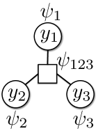
When , differences start to become apparent. In this setting both models have six parameters: for the DPP they are , and for the MRF they are . To place the two models on equal footing, we represent each as the product of unnormalized per-item potentials and a single unnormalized ternary potential . This representation corresponds to a factor graph with three nodes and a single, ternary factor (see Figure 10). The probability of a set is then given by
| (103) |
For the DPP, the node potentials are , and for the MRF they are . The ternary factors are
| (104) | ||||
| (105) |
| {} | 000 | 1 | 1 |
|---|---|---|---|
| {1} | 100 | 1 | 1 |
| {2} | 010 | 1 | 1 |
| {3} | 001 | 1 | 1 |
| {1,2} | 110 | ||
| {1,3} | 101 | ||
| {2,3} | 011 | ||
| {1,2,3} | 111 |
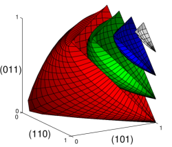
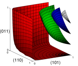
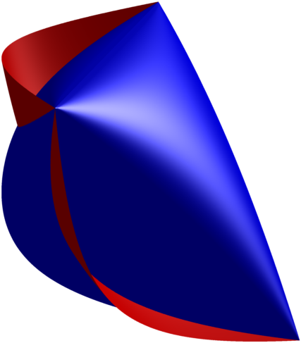
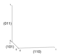
Since both models allow setting the node potentials arbitrarily, we focus now on the ternary factor. Table 1 shows the values of and for all subsets . The last four entries are determined, respectively, by the three edge parameters of the MRF and three similarity parameters of the DPP, so the sets of realizable ternary factors form 3-D manifolds in 4-D space. We attempt to visualize these manifolds by showing 2-D slices in 3-D space for various values of (the last row of Table 1).
Figure 11a depicts four such slices of the realizable DPP distributions, and Figure 11b shows the same slices of the realizable MRF distributions. Points closer to the origin (on the lower left) correspond to “more repulsive” distributions, where the three elements of are less likely to appear together. When is large (gray surfaces), negative correlations are weak and the two models give rise to qualitatively similar distributions. As the value of the shrinks to zero (red surfaces), the two models become quite different. MRFs, for example, can describe distributions where the first item is strongly anti-correlated with both of the others, but the second and third are not anti-correlated with each other. The transitive nature of the DPP makes this impossible.
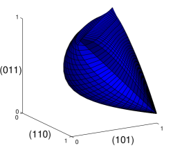
To improve visibility, we have constrained in Figure 11a. Figure 11c shows a single slice without this constraint; allowing negative similarity makes it possible to achieve strong three-way repulsion with less pairwise repulsion, closing the surface away from the origin. The corresponding MRF slice is shown in Figure 11d, and the two are overlaid in Figure 11e and Figure 11f. Even though there are relatively strong interactions in these plots (), the models remain roughly comparable in terms of the distributions they can express.
As gets larger, we conjecture that the story is essentially the same. DPPs are primarily constrained by a notion of transitivity on the similarity measure; thus it would be difficult to use a DPP to model, for example, data where items repel “distant” items rather than similar items—if is far from and is far from we cannot necessarily conclude that is far from . One way of looking at this is that repulsion of distant items induces positive correlations between the selected items, which a DPP cannot represent.
MRFs, on the other hand, are constrained by their local nature and do not effectively model data that are “globally” diverse. For instance, a pairwise MRF we cannot exclude a set of three or more items without excluding some pair of those items. More generally, an MRF assumes that repulsion does not depend on (too much) context, so it cannot express that, say, there can be only a certain number of selected items overall. The DPP can naturally implement this kind of restriction though the rank of the kernel.
3.3 Dual representation
The standard inference algorithms for DPPs rely on manipulating the kernel through inversion, eigendecomposition, and so on. However, in situations where is large we may not be able to work efficiently with —in some cases we may not even have the memory to write it down. In this section, instead, we develop a dual representation of a DPP that shares many important properties with the kernel but is often much smaller. Afterwards, we will show how this dual representation can be applied to perform efficient inference.
Let be the matrix whose columns are given by , so that . Consider now the matrix
| (106) |
By construction, is symmetric and positive semidefinite. In contrast to , which is too expensive to work with when is large, is only , where is the dimension of the diversity feature function . In many practical situations, is fixed by the model designer, while may grow without bound as new items become available; for instance, a search engine may continually add to its database of links. Furthermore, we have the following result.
Proposition 3.1.
The nonzero eigenvalues of and are identical, and the corresponding eigenvectors are related by the matrix . That is,
| (107) |
is an eigendecomposition of if and only if
| (108) |
is an eigendecomposition of .
Proof.
In the forward direction, we assume that is an eigendecomposition of . We have
| (109) | ||||
| (110) |
since are orthonormal by assumption. Furthermore, for any we have
| (111) | ||||
| (112) | ||||
| (113) | ||||
| (114) |
using the fact that since is an eigenvector of . Finally, for any distinct , we have
| (115) | ||||
| (116) | ||||
| (117) |
Thus is an eigendecomposition of . In the other direction, an analogous argument applies once we observe that, since , has rank at most and therefore at most nonzero eigenvalues. ∎
Proposition 3.1 shows that contains quite a bit of information about . In fact, is sufficient to perform nearly all forms of DPP inference efficiently, including normalization and marginalization in constant time with respect to , and sampling in time linear in .
3.3.1 Normalization
Recall that the normalization constant for a DPP is given by . If are the eigenvalues of , then the normalization constant is equal to , since the determinant is the product of the eigenvalues of its argument. By Proposition 3.1, the nonzero eigenvalues of are also the eigenvalues of the dual representation . Thus, we have
| (118) |
Computing the determinant of requires time.
3.3.2 Marginalization
Standard DPP marginalization makes use of the marginal kernel , which is of course as large as . However, the dual representation can be used to compute the entries of . We first eigendecompose the dual representation as , which requires time. Then, we can use the definition of in terms of the eigendecomposition of as well as Proposition 3.1 to compute
| (119) | ||||
| (120) |
That is, the diagonal entries of are computable from the dot products between the diversity features and the eigenvectors of ; we can therefore compute the marginal probability of a single item from an eigendecomposition of in time. Similarly, given two items and we have
| (121) | ||||
| (122) |
so we can compute arbitrary entries of in time. This allows us to compute, for example, pairwise marginals . More generally, for a set , , we need to compute entries of to obtain , and taking the determinant then yields . The process requires only time; for small sets this is just quadratic in the dimension of .
3.3.3 Sampling
Recall the DPP sampling algorithm, which is reproduced for convenience in Algorithm 2. We will show that this algorithm can be implemented in a tractable manner by using the dual representation . The main idea is to represent , the orthonormal set of vectors in , as a set of vectors in , with the mapping
| (123) |
Note that, when contains eigenvectors of , this is (up to scale) the relationship established by Proposition 3.1 between eigenvectors of and eigenvectors of .
The mapping in Equation (123) has several useful properties. If and , then , and likewise for any arbitrary linear combination. In other words, we can perform implicit scaling and addition of the vectors in using only their preimages in . Additionally, we have
| (124) | ||||
| (125) |
so we can compute dot products of vectors in in time. This means that, for instance, we can implicitly normalize by updating .
We now show how these operations allow us to efficiently implement key parts of the sampling algorithm. Because the nonzero eigenvalues of and are equal, the first loop of the algorithm, where we choose in index set , remains unchanged. Rather than using to construct orthonormal directly, however, we instead build the set by adding for every .
In the last phase of the loop, we need to find an orthonormal basis for the subspace of orthogonal to a given . This requires two steps. In the first, we subtract a multiple of one of the vectors in from all of the other vectors so that they are zero in the th component, leaving us with a set of vectors spanning the subspace of orthogonal to . In order to do this we must be able to compute the th component of a vector ; since , this is easily done by computing the th column of , and then taking the dot product with . This takes only time. In the second step, we use the Gram-Schmidt process to convert the resulting vectors into an orthonormal set. This requires a series of dot products, sums, and scalings of vectors in ; however, as previously argued all of these operations can be performed implicitly. Therefore the mapping in Equation (123) allows us to implement the final line of the second loop using only tractable computations on vectors in .
All that remains, then, is to efficiently choose an item according to the distribution
| (126) | ||||
| (127) |
in the first line of the while loop. Simplifying, we have
| (128) |
Thus the required distribution can be computed in time , where . The complete dual sampling algorithm is given in Algorithm 3; the overall runtime is .
3.4 Random projections
As we have seen, dual DPPs allow us to deal with settings where is too large to work efficiently with by shifting the computational focus to the dual kernel , which is only . This is an effective approach when . Of course, in some cases might also be unmanageably large, for instance when the diversity features are given by word counts in natural language settings, or high-resolution image features in vision.
To address this problem, we describe a method for reducing the dimension of the diversity features while maintaining a close approximation to the original DPP model. Our approach is based on applying random projections, an extremely simple technique that nonetheless provides an array of theoretical guarantees, particularly with respect to preserving distances between points (Vempala, 2004). A classic result of Johnson and Lindenstrauss (1984), for instance, shows that high-dimensional points can be randomly projected onto a logarithmic number of dimensions while approximately preserving the distances between them. More recently, Magen and Zouzias (2008) extended this idea to the preservation of volumes spanned by sets of points. Here, we apply the connection between DPPs and spanned volumes to show that random projections allow us to reduce the dimensionality of , dramatically speeding up inference, while maintaining a provably close approximation to the original, high-dimensional model. We begin by stating a variant of Magen and Zouzias’ result.
Lemma 3.2.
(Adapted from Magen and Zouzias (2008)) Let be a matrix. Fix and , and set the projection dimension
| (129) |
Let be a random projection matrix whose entries are independently sampled from , and let , where , denote the matrix formed by taking the columns of corresponding to indices in . Then with probability at least we have, for all with cardinality at most :
| (130) |
where is the -dimensional volume of the parallelepiped spanned by the columns of .
Lemma 3.2 says that, with high probability, randomly projecting to
| (131) |
dimensions is sufficient to approximately preserve all volumes spanned by columns of . We can use this result to bound the effectiveness of random projections for DPPs.
In order to obtain a result that is independent of , we will restrict ourselves to the portion of the distribution pertaining to subsets with cardinality at most a constant . This restriction is intuitively reasonable for any application where we use DPPs to model sets of relatively small size compared to , which is common in practice. However, formally it may seem a bit strange, since it implies conditioning the DPP on cardinality. In Section 5 we will show that this kind of conditioning is actually very practical and efficient, and Theorem 3.3, which we prove shortly, will apply directly to the -DPPs of Section 5 without any additional work.
For now, we will seek to approximate the distribution , which is simply the original DPP conditioned on the cardinality of the modeled subset:
| (132) |
where denotes the matrix formed from columns for . Our main result follows.
Theorem 3.3.
Let be the cardinality-conditioned DPP distribution defined by quality model and -dimensional diversity feature function , and let
| (133) |
be the cardinality-conditioned DPP distribution obtained by projecting with . Then for projection dimension as in Equation (129), we have
| (134) |
with probability at least . Note that when is small.
The theorem says that for logarithmic in and linear in , the variational distance between the original DPP and the randomly projected version is bounded. In order to use Lemma 3.2, which bounds volumes of parallelepipeds, to prove this bound on determinants, we will make use of the following relationship:
| (135) |
In order to handle the conditional DPP normalization constant
| (136) |
we also must adapt Lemma 3.2 to sums of determinants. Finally, for technical reasons we will change the symmetry of the upper and lower bounds from the sign of to the sign of the exponent. The following lemma gives the details.
Lemma 3.4.
Under the definitions and assumptions of Lemma 3.2, we have, with probability at least ,
| (137) |
Proof.
| (138) | ||||
| (139) | ||||
| (140) | ||||
| (141) |
where the first inequality holds with probability at least by Lemma 3.2, and the third follows from the fact that (since ), thus . The upper bound follows directly:
| (142) | ||||
| (143) |
∎
We can now prove Theorem 3.3.
Proof of Theorem 3.3.
By combining the dual representation with random projections, we can deal simultaneously with very large and very large . In fact, in Section 6 we will show that can even be exponentially large if certain structural assumptions are met. These techniques vastly expand the range of problems to which DPPs can be practically applied.
3.5 Alternative likelihood formulas
Recall that, in an L-ensemble DPP, the likelihood of a particular set is given by
| (148) |
This expression has some nice intuitive properties in terms of volumes, and, ignoring the normalization in the denominator, takes a simple and concise form. However, as a ratio of determinants on matrices of differing dimension, it may not always be analytically convenient. Minors can be difficult to reason about directly, and ratios complicate calculations like derivatives. Moreover, we might want the likelihood in terms of the marginal kernel , but simply plugging in these identities yields a expression that is somewhat unwieldy.
As alternatives, we will derive some additional formulas that, depending on context, may have useful advantages. Our starting point will be the observation, used previously in the proof of Theorem 21, that minors can be written in terms of full matrices and diagonal indicator matrices; specifically, for positive semidefinite ,
| (149) | ||||
| (150) | ||||
| (151) |
where is the diagonal matrix with ones in the diagonal positions corresponding to elements of and zeros everywhere else, and . These identities can be easily shown by examining the matrices blockwise under the partition , as in the proof of Theorem 21.
Applying Equation (149) to Equation (148), we get
| (152) | ||||
| (153) | ||||
| (154) |
Already, this expression, which is a single determinant of an matrix, is in some ways easier to work with. We can also more easily write the likelihood in terms of :
| (155) |
Recall from Equation (35) that is the marginal kernel of the complement DPP; thus, in an informal sense we can read Equation (155) as combining the marginal probability that is selected with the marginal probability that is not selected.
4 Learning
We have seen that determinantal point process offer appealing modeling intuitions and practical algorithms, capturing geometric notions of diversity and permitting computationally efficient inference in a variety of settings. However, to accurately model real-world data we must first somehow determine appropriate values of the model parameters. While an expert could conceivably design an appropriate DPP kernel from prior knowledge, in general, especially when dealing with large data sets, we would like to have an automated method for learning a DPP.
We first discuss how to parameterize DPPs conditioned on input data. We then define what we mean by learning, and, using the quality vs. diversity decomposition introduced in Section 3.1, we show how a parameterized quality model can be learned efficiently from a training set.
4.1 Conditional DPPs
Suppose we want to use a DPP to model the seats in an auditorium chosen by students attending a class. (Perhaps we think students tend to spread out.) In this context each meeting of the class is a new sample from the empirical distribution over subsets of the (fixed) seats, so we merely need to collect enough samples and we should be able to fit our model, as desired.
For many problems, however, the notion of a single fixed base set is inadequate. For instance, consider extractive document summarization, where the goal is to choose a subset of the sentences in a news article that together form a good summary of the entire article. In this setting is the set of sentences in the news article being summarized, thus is not fixed in advance but instead depends on context. One way to deal with this problem is to model the summary for each article as its own DPP with a separate kernel matrix. This approach certainly affords great flexibility, but if we have only a single sample summary for each article, there is little hope of getting good parameter estimates. Even more importantly, we have learned nothing that can be applied to generate summaries of unseen articles at test time, which was presumably our goal in the first place.
Alternatively, we could let be the set of all sentences appearing in any news article; this allows us to learn a single model for all of our data, but comes with obvious computational issues and does not address the other concerns, since sentences are rarely repeated.
To solve this problem, we need a DPP that depends parametrically on the input data; this will enable us to share information across training examples in a justifiable and effective way. We first introduce some notation. Let be the input space; for example, might be the space of news articles. Let denote the ground set of items implied by an input , e.g., the set of all sentences in news article . We have the following definition.
Definition 4.1.
A conditional DPP is a conditional probabilistic model which assigns a probability to every possible subset . The model takes the form of an L-ensemble:
| (162) |
where is a positive semidefinite kernel matrix that depends on the input.
As discussed in Section 2, the normalization constant for a conditional DPP can be computed efficiently and is given by . Using the quality/diversity decomposition introduced in Section 3.1, we have
| (163) |
for suitable and , , which now depend on .
In the following sections we will discuss application-specific parameterizations of the quality and diversity models and in terms of the input. First, however, we review our learning setup.
4.1.1 Supervised learning
The basic supervised learning problem is as follows. We receive a training data sample drawn independently and identically from a distribution over pairs , where is an input space and is the associated ground set for input . We assume that the conditional DPP kernel is parameterized in terms of a generic , and let
| (164) |
denote the conditional probability of an output given input under parameter . The goal of learning is to choose appropriate based on the training sample so that we can make accurate predictions on unseen inputs.
While there are a variety of objective functions commonly used for learning, here we will focus on maximum likelihood learning (or maximum likelihood estimation, often abbreviated MLE), where the goal is to choose to maximize the conditional log-likelihood of the observed data:
| (165) | ||||
| (166) | ||||
| (167) |
Optimizing is consistent under mild assumptions; that is, if the training data are actually drawn from a conditional DPP with parameter , then the learned as . Of course real data are unlikely to exactly follow any particular model, but in any case the maximum likelihood approach has the advantage of calibrating the DPP to produce reasonable probability estimates, since maximizing can be seen as minimizing the log-loss on the training data.
To optimize the log-likelihood, we will use standard algorithms such as gradient ascent or L-BFGS (Nocedal, 1980). These algorithms depend on the gradient , which must exist and be computable, and they converge to the optimum whenever is concave in . Thus, our ability to optimize likelihood efficiently will depend fundamentally on these two properties.
4.2 Learning quality
We begin by showing how to learn a parameterized quality model when the diversity feature function is held fixed (Kulesza and Taskar, 2011b). This setup is somewhat analogous to support vector machines (Vapnik, 2000), where a kernel is fixed by the practitioner and then the per-example weights are automatically learned. Here, can consist of any desired measurements (and could even be infinite-dimensional, as long as the resulting similarity matrix is a proper kernel). We propose computing the quality scores using a log-linear model:
| (168) |
where is a feature vector for item and the parameter is now concretely an element of . Note that feature vectors are in general distinct from ; the former are used for modeling quality, and will be “interpreted” by the parameters , while the latter define the diversity model , which is fixed in advance. We have
| (169) |
For ease of notation, going forward we will assume that the training set contains only a single instance , and drop the instance index . All of the following results extend easily to multiple training examples. First, we show that under this parameterization the log-likelihood function is concave in ; then we will show that its gradient can be computed efficiently. With these results in hand we will be able to apply standard optimization techniques.
Proposition 4.2.
is concave in .
Proof.
We have
| (170) | ||||
| (171) |
With respect to , the first term is linear, the second is constant, and the third is the composition of a concave function (negative log-sum-exp) and an affine function, so the overall expression is concave. ∎
We now derive the gradient , using Equation (171) as a starting point.
| (172) | ||||
| (173) | ||||
| (174) |
Thus, as in standard maximum entropy modeling, the gradient of the log-likelihood can be seen as the difference between the empirical feature counts and the expected feature counts under the model distribution. The difference here, of course, is that is a DPP, which assigns higher probability to diverse sets. Compared with a standard independent model obtained by removing the diversity term from , Equation (174) actually emphasizes those training examples that are not diverse, since these are the examples on which the quality model must focus its attention in order to overcome the bias imposed by the determinant. In the experiments that follow we will see that this distinction is important in practice.
The sum over in Equation (174) is exponential in ; hence we cannot compute it directly. Instead, we can rewrite it by switching the order of summation:
| (175) |
Note that is the marginal probability of item appearing in a set sampled from the conditional DPP. That is, the expected feature counts are computable directly from the marginal probabilities. Recall that we can efficiently marginalize DPPs; in particular, per-item marginal probabilities are given by the diagonal of , the marginal kernel (which now depends on the input and the parameters). We can compute from the kernel using matrix inversion or eigendecomposition. Algorithm 4 shows how we can use these ideas to compute the gradient of efficiently.
In fact, note that we do not need all of , but only its diagonal. In Algorithm 4 we exploit this in the main loop, using only multiplications rather than the we would need to construct the entire marginal kernel. (In the dual representation, this can be improved further to multiplications.) Unfortunately, these savings are asymptotically irrelevant since we still need to eigendecompose , requiring about time (or time for the corresponding eigendecomposition in the dual). It is conceivable that a faster algorithm exists for computing the diagonal of directly, along the lines of ideas recently proposed by Tang and Saad (2011) (which focus on sparse matrices); however, we are not currently aware of a useful improvement over Algorithm 4.
4.2.1 Experiments: document summarization
We demonstrate learning for the conditional DPP quality model on an extractive multi-document summarization task using news text. The basic goal is to generate a short piece of text that summarizes the most important information from a news story. In the extractive setting, the summary is constructed by stringing together sentences found in a cluster of relevant news articles. This selection problem is a balancing act: on the one hand, each selected sentence should be relevant, sharing significant information with the cluster as a whole; on the other, the selected sentences should be diverse as a group so that the summary is not repetitive and is as informative as possible given its length (Dang, 2005; Nenkova et al., 2006). DPPs are a natural fit for this task, viewed through the decomposition of Section 3.1 (Kulesza and Taskar, 2011b).
As in Section 4.1, the input will be a cluster of documents, and a set of candidate sentences from those documents. In our experiments contains all sentences from all articles in the cluster, although in general preprocessing could also be used to try to improve the candidate set (Conroy et al., 2004). We will learn a DPP to model good summaries for a given input . Because DPPs model unordered sets while summaries are linear text, we construct a written summary from by placing the sentences it contains in the same order in which they appeared in the original documents. This policy is unlikely to give optimal results, but it is consistent with prior work (Lin and Bilmes, 2010) and seems to perform well. Furthermore, it is at least partially justified by the fact that modern automatic summary evaluation metrics like ROUGE, which we describe later, are mostly invariant to sentence order.
We experiment with data from the multi-document summarization task (Task 2) of the 2003 and 2004 Document Understanding Conference (DUC) (Dang, 2005). The article clusters used for these tasks are taken from the NIST TDT collection. Each cluster contains approximately 10 articles drawn from the AP and New York Times newswires, and covers a single topic over a short time span. The clusters have a mean length of approximately 250 sentences and 5800 words. The 2003 task, which we use for training, contains 30 clusters, and the 2004 task, which is our test set, contains 50 clusters. Each cluster comes with four reference human summaries (which are not necessarily formed by sentences from the original articles) for evaluation purposes. Summaries are required to be at most 665 characters in length, including spaces. Figure 12 depicts a sample cluster from the test set.

To measure performance on this task we follow the original evaluation and use ROUGE, an automatic evaluation metric for summarization (Lin, 2004). ROUGE measures -gram overlap statistics between the human references and the summary being scored, and combines them to produce various sub-metrics. ROUGE-1, for example, is a simple unigram recall measure that has been shown to correlate quite well with human judgments (Lin, 2004). Here, we use ROUGE’s unigram F-measure (which combines ROUGE-1 with a measure of precision) as our primary metric for development. We refer to this measure as ROUGE-1F. We also report ROUGE-1P and ROUGE-1R (precision and recall, respectively) as well as ROUGE-2F and ROUGE-SU4F, which include bigram match statistics and have also been shown to correlate well with human judgments. Our implementation uses ROUGE version 1.5.5 with stemming turned on, but without stopword removal. These settings correspond to those used for the actual DUC competitions (Dang, 2005); however, we use a more recent version of ROUGE.
Training data
Recall that our learning setup requires a training sample of pairs , where . Unfortunately, while the human reference summaries provided with the DUC data are of high quality, they are not extractive, thus they do not serve as examples of summaries that we can actually model. To obtain high-quality extractive “oracle” summaries from the human summaries, we employ a simple greedy algorithm (Algorithm 5). On each round the sentence that achieves maximal unigram F-measure to the human references, normalized by length, is selected and added to the extractive summary. Since high F-measure requires high precision as well as recall, we then update the references by removing the words “covered” by the newly selected sentence, and proceed to the next round.
We can measure the success of this approach by calculating ROUGE scores of our oracle summaries with respect to the human summaries. Table 2 shows the results for the DUC 2003 training set. For reference, the table also includes the ROUGE scores of the best automatic system from the DUC competition in 2003 (“machine”), as well as the human references themselves (“human”). Note that, in the latter case, the human summary being evaluated is also one of the four references used to compute ROUGE; hence the scores are probably significantly higher than a human could achieve in practice. Furthermore, it has been shown that extractive summaries, even when generated optimally, are by nature limited in quality compared with unconstrained summaries (Genest et al., 2010). Thus we believe that the oracle summaries make strong targets for training.
| System | ROUGE-1F | ROUGE-2F | ROUGE-SU4F |
|---|---|---|---|
| Machine | 35.17 | 9.15 | 12.47 |
| Oracle | 46.59 | 16.18 | 19.52 |
| Human | 56.22 | 33.37 | 36.50 |
Features
We next describe the feature functions that we use for this task. For diversity features , we generate standard normalized tf-idf vectors. We tokenize the input test, remove stop words and punctuation, and apply a Porter stemmer.222Code for this preprocessing pipeline was provided by Hui Lin and Jeff Bilmes. Then, for each word , the term frequency of in sentence is defined as the number of times the word appears in the sentence, and the inverse document frequency is the negative logarithm of the fraction of articles in the training set where appears. A large value of implies that is relatively rare. Finally, the vector has one element per word, and the value of the entry associated with word is proportional to . The scale of is set such that .
Under this definition of , the similarity between sentences and is known as their cosine similarity:
| (176) |
Two sentences are cosine similar if they contain many of the same words, particularly words that are uncommon (and thus more likely to be salient).
We augment with an additional constant feature taking the value , which is a hyperparameter. This has the effect of making all sentences more similar to one another, increasing repulsion. We set to optimize ROUGE-1F score on the training set; in our experiments, the best choice was .
We use the very standard cosine distance as our similarity metric because we need to be confident that it is sensible; it will remain fixed throughout the experiments. On the other hand, weights for the quality features are learned, so we can use a variety of intuitive measures and rely on training to find an appropriate combination. The quality features we use are listed below. For some of the features, we make use of cosine distances; these are computed using the same tf-idf vectors as the diversity features. When a feature is intrinsically real-valued, we produce a series of binary features by binning. The bin boundaries are determined either globally or locally. Global bins are evenly spaced quantiles of the feature values across all sentences in the training set, while local bins are quantiles of the feature values in the current cluster only.
-
•
Constant: A constant feature allows the model to bias towards summaries with a greater or smaller number of sentences.
-
•
Length: We bin the length of the sentence (in characters) into five global bins.
-
•
Document position: We compute the position of the sentence in its original document and generate binary features indicating positions 1–5, plus a sixth binary feature indicating all other positions. We expect that, for newswire text, sentences that appear earlier in an article are more likely to be useful for summarization.
-
•
Mean cluster similarity: For each sentence we compute the average cosine distance to all other sentences in the cluster. This feature attempts to measure how well the sentence reflects the salient words occurring most frequently in the cluster. We use the raw score, five global bins, and ten local bins.
-
•
LexRank: We compute continuous LexRank scores by finding the principal eigenvector of the row-normalized cosine similarity matrix. (See Erkan and Radev (2004) for details.) This provides an alternative measure of centrality. We use the raw score, five global bins, and five local bins.
-
•
Personal pronouns: We count the number of personal pronouns (“he”, “her”, “themselves”, etc.) appearing in each sentence. Sentences with many pronouns may be poor for summarization since they omit important entity names.
In total we have 40 quality features; including our model has 41 parameters.
Inference
At test time, we need to take the learned parameters and use them to predict a summary for a previously unseen document cluster . One option is to sample from the conditional distribution, which can be done exactly and efficiently, as described in Section 2.4.4. However, sampling occasionally produces low-probability predictions. We obtain better performance on this task by applying two alternative inference techniques.
Greedy MAP approximation. One common approach to prediction in probabilistic models is maximum a posteriori (MAP) decoding, which selects the highest probability configuration. For practical reasons, and because the primary metrics for evaluation were recall-based, the DUC evaluations imposed a length limit of 665 characters, including spaces, on all summaries. In order to compare with prior work we also apply this limit in our tests. Thus, our goal is to find the most likely summary, subject to a budget constraint:
| (177) |
where is the number of characters in sentence , and is the limit on the total length. As discussed in Section 2.4.5, computing exactly is NP-hard, but, recalling that the optimization in Equation (177) is submodular, we can approximate it through a simple greedy algorithm (Algorithm 6).
Algorithm 6 is closely related to those given by Krause and Guestrin (2005) and especially Lin and Bilmes (2010). As discussed in Section 2.4.5, algorithms of this type have formal approximation guarantees for monotone submodular problems. Our MAP problem is not generally monotone; nonetheless, Algorithm 6 seems to work well in practice, and is very fast (see Table 3).
Minimum Bayes risk decoding. The second inference technique we consider is minimum Bayes risk (MBR) decoding. First proposed by Goel and Byrne (2000) for automatic speech recognition, MBR decoding has also been used successfully for word alignment and machine translation (Kumar and Byrne, 2002, 2004). The idea is to choose a prediction that minimizes a particular application-specific loss function under uncertainty about the evaluation target. In our setting we use ROUGE-1F as a (negative) loss function, so we have
| (178) |
where the expectation is over realizations of , the true summary against which we are evaluated. Of course, the distribution of is unknown, but we can assume that our trained model gives a reasonable approximation. Since there are exponentially many possible summaries, we cannot expect to perform an exact search for ; however, we can approximate it through sampling, which is efficient.
Combining these approximations, we have the following inference rule:
| (179) |
where are samples drawn from . In order to satisfy the length constraint imposed by the evaluation, we consider only samples with length between 660 and 680 characters (rejecting those that fall outside this range), and crop to the limit of 665 bytes if necessary. The choice of is a tradeoff between fast running time and quality of inference. In the following section, we report results for and ; Table 3 shows the average time required to produce a summary under each setting. Note that MBR decoding is easily parallelizable, but the results in Table 3 are for a single processor. Since MBR decoding is randomized, we report all results averaged over 100 trials.
| System | Time (s) | |
|---|---|---|
| dpp-greedy | 0. | 15 |
| dpp-mbr100 | 1. | 30 |
| dpp-mbr1000 | 16. | 91 |
| dpp-mbr5000 | 196. | 86 |
Results
We train our model with a standard L-BFGS optimization algorithm. We place a zero-mean Gaussian prior on the parameters , with variance set to optimize ROUGE-1F on a development subset of the 2003 data. We learn parameters on the DUC 2003 corpus, and test them using DUC 2004 data. We generate predictions from the trained DPP using the two inference algorithms described in the previous section, and compare their performance to a variety of baseline systems.
Our first and simplest baseline merely returns the first 665 bytes of the cluster text. Since the clusters consist of news articles, this is not an entirely unreasonable summary in many cases. We refer to this baseline as begin.
We also compare against an alternative DPP-based model with identical similarity measure and quality features, but where the quality model has been trained using standard logistic regression. To learn this baseline, each sentence is treated as a unique instance to be classified as included or not included, with labels derived from our training oracle. Thus, it has the advantages of a DPP at test time, but does not take into account the diversity model while training; comparing to this baseline allows us to isolate the contribution of learning the model parameters in context. Note that MBR inference is impractical for this model because its training does not properly calibrate for overall summary length, so nearly all samples are either too long or too short. Thus, we report only the results obtained from greedy inference. We refer to this model as lr+dpp.
Next, we employ as baselines a range of previously proposed methods for multi-document summarization. Perhaps the simplest and most popular is Maximum Marginal Relevance (MMR), which uses a greedy selection process (Carbonell and Goldstein, 1998). MMR relies on a similarity measure between sentences, for which we use the cosine distance measure , and a measure of relevance for each sentence, for which we use the same logistic regression-trained quality model as above. Sentences are chosen iteratively according to
| (180) |
where is the set of sentences already selected (initially empty), is the learned quality score, and is the cosine similarity between sentences and . The tradeoff is optimized on a development set, and sentences are added until the budget is full. We refer to this baseline as lr+mmr.
We also compare against the three highest-scoring systems that actually competed in the DUC 2004 competition—peers 65, 104, and 35—as well as the submodular graph-based approach recently described by Lin and Bilmes (2010), which we refer to as submod1, and the improved submodular learning approach proposed by Lin and Bilmes (2012), which we denote submod2. We produced our own implementation of submod1, but rely on previously reported numbers for submod2, which include only ROUGE-1 scores.
Table 4 shows the results for all methods on the DUC 2004 test corpus. Scores for the actual DUC competitors differ slightly from the originally reported results because we use an updated version of the ROUGE package. Bold entries highlight the best performance in each column; in the case of MBR inference, which is stochastic, the improvements are significant at 99% confidence. The DPP models outperform the baselines in most cases; furthermore, there is a significant boost in performance due to the use of DPP maximum likelihood training in place of logistic regression. MBR inference performs best, assuming we take sufficiently many samples; on the other hand, greedy inference runs more quickly than dpp-mbr100 and produces superior results. Relative to most other methods, the DPP model with MBR inference seems to more strongly emphasize recall. Note that MBR inference was performed with respect to ROUGE-1F, but could also be run to optimize other metrics if desired.
| System | ROUGE-1F | ROUGE-1P | ROUGE-1R | ROUGE-2F | ROUGE-SU4F |
|---|---|---|---|---|---|
| begin | 32.08 | 31.53 | 32.69 | 6.52 | 10.37 |
| lr+mmr | 37.58 | 37.15 | 38.05 | 9.05 | 13.06 |
| lr+dpp | 37.96 | 37.67 | 38.31 | 8.88 | 13.13 |
| peer 35 | 37.54 | 37.69 | 37.45 | 8.37 | 12.90 |
| peer 104 | 37.12 | 36.79 | 37.48 | 8.49 | 12.81 |
| peer 65 | 37.87 | 37.58 | 38.20 | 9.13 | 13.19 |
| submod1 | 38.73 | 38.40 | 39.11 | 8.86 | 13.11 |
| submod2 | 39.78 | 39.16 | 40.43 | - | - |
| dpp-greedy | 38.96 | 38.82 | 39.15 | 9.86 | 13.83 |
| dpp-mbr100 | 38.83 | 38.06 | 39.67 | 8.85 | 13.38 |
| dpp-mbr1000 | 39.79 | 38.96 | 40.69 | 9.29 | 13.87 |
| dpp-mbr5000 | 40.33 | 39.43 | 41.31 | 9.54 | 14.13 |
Feature contributions. In Table 5 we report the performance of dpp-greedy when different groups of features from Section 4.2.1 are removed, in order to estimate their relative contributions. Length and position appear to be quite important; however, although individually similarity and LexRank scores have only a modest impact on performance, when both are omitted the drop is significant. This suggests, intuitively, that these two groups convey similar information—both are essentially measures of centrality—but that this information is important to achieving strong performance.
| Features | ROUGE-1F | ROUGE-1P | ROUGE-1R |
|---|---|---|---|
| All | 38.96 | 38.82 | 39.15 |
| All but length | 37.38 | 37.08 | 37.72 |
| All but position | 36.34 | 35.99 | 36.72 |
| All but similarity | 38.14 | 37.97 | 38.35 |
| All but LexRank | 38.10 | 37.92 | 38.34 |
| All but pronouns | 38.80 | 38.67 | 38.98 |
| All but similarity, LexRank | 36.06 | 35.84 | 36.32 |
5 -DPPs
A determinantal point process assigns a probability to every subset of the ground set . This means that, with some probability, a sample from the process will be empty; with some probability, it will be all of . In many cases this is not desirable. For instance, we might want to use a DPP to model the positions of basketball players on a court, under the assumption that a team tends to spread out for better coverage. In this setting, we know that with very high probability each team will have exactly five players on the court. Thus, if our model gives some probability of seeing zero or fifty players, it is not likely to be a good fit.
We showed in Section 2.4.4 that there exist elementary DPPs having fixed cardinality ; however, this is achieved only by focusing exclusively (and equally) on specific “aspects” of the data, as represented by eigenvectors of the kernel. Thus, for DPPs, the notions of size and content are fundamentally intertwined. We cannot change one without affecting the other. This is a serious limitation on the types of distributions than can be expressed; for instance, a DPP cannot even capture the uniform distribution over sets of cardinality .
More generally, even for applications where the number of items is unknown, the size model imposed by a DPP may not be a good fit. We have seen that the cardinality of a DPP sample has a simple distribution: it is the number of successes in a series of Bernoulli trials. But while this distribution characterizes certain types of data, other cases might look very different. For example, picnickers may tend to stake out diverse positions in a park, but on warm weekend days there might be hundreds of people, and on a rainy Tuesday night there are likely to be none. This bimodal distribution is quite unlike the sum of Bernoulli variables imposed by DPPs.
Perhaps most importantly, in some cases we do not even want to model cardinality at all, but instead offer it as a parameter. For example, a search engine might need to deliver ten diverse results to its desktop users, but only five to its mobile users. This ability to control the size of a DPP “on the fly” can be crucial in real-world applications.
In this section we introduce -DPPs, which address the issues described above by conditioning a DPP on the cardinality of the random set . This simple change effectively divorces the DPP content model, with its intuitive diversifying properties, from the DPP size model, which is not always appropriate. We can then use the DPP content model with a size model of our choosing, or simply set the desired size based on context. The result is a significantly more expressive modeling approach (which can even have limited positive correlations) and increased control.
We begin by defining -DPPs. The conditionalization they require, though simple in theory, necessitates new algorithms for inference problems like normalization and sampling. Naively, these tasks require exponential time, but we show that through recursions for computing elementary symmetric polynomials we can solve them exactly in polynomial time. Finally, we demonstrate the use of -DPPs on an image search problem, where the goal is to show users diverse sets of images that correspond to their query.
5.1 Definition
A -DPP on a discrete set is a distribution over all subsets with cardinality (Kulesza and Taskar, 2011a). In contrast to the standard DPP, which models both the size and content of a random subset , a -DPP is concerned only with the content of a random -set. Thus, a -DPP is obtained by conditioning a standard DPP on the event that the set has cardinality . Formally, the -DPP gives probabilities
| (181) |
where and is a positive semidefinite kernel. Compared to the standard DPP, the only changes are the restriction on and the normalization constant. While in a DPP every -set competes with all other subsets of , in a -DPP it competes only with sets of the same cardinality. This subtle change has significant implications.
For instance, consider the seemingly simple distribution that is uniform over all sets with cardinality . If we attempt to build a DPP capturing this distribution we quickly run into difficulties. In particular, the marginal probability of any single item is , so the marginal kernel , if it exists, must have on the diagonal. Likewise, the marginal probability of any pair of items is , and so by symmetry the off diagonal entries of must be equal to a constant. As a result, any valid marginal kernel has to be the sum of a constant matrix and a multiple of the identity matrix. Since a constant matrix has at most one nonzero eigenvalue and the identity matrix is full rank, it is easy to show that, except in the special cases , the resulting kernel has full rank. But we know that a full rank kernel implies that the probability of seeing all items together is nonzero. Thus the desired process cannot be a DPP unless or . On the other hand, a -DPP with the identity matrix as its kernel gives the distribution we are looking for. This improved expressive power can be quite valuable in practice.
5.1.1 Alternative models of size
Since a -DPP is conditioned on cardinality, must come from somewhere outside of the model. In many cases, may be fixed according to application needs, or perhaps changed on the fly by users or depending on context. This flexibility and control is one of the major practical advantages of -DPPs. Alternatively, in situations where we wish to model size as well as content, a -DPP can be combined with a size model that assigns a probability to every possible :
| (182) |
Since the -DPP is a proper conditional model, the distribution is well-defined. By choosing appropriate to the task at hand, we can effectively take advantage of the diversifying properties of DPPs in situations where the DPP size model is a poor fit.
As a side effect, this approach actually enables us to use -DPPs to build models with both negative and positive correlations. For instance, if indicates that there are likely to be either hundreds of picnickers in the park (on a nice day) or, otherwise, just a few, then knowing that there are fifty picnickers today implies that there are likely to be even more. Thus, -DPPs can yield more expressive models than DPPs in this sense as well.
5.2 Inference
Of course, increasing the expressive power of the DPP causes us to wonder whether, in doing so, we might have lost some of the convenient computational properties that made DPPs useful in the first place. Naively, this seems to be the case; for instance, while the normalizing constant for a DPP can be written in closed form, the sum in Equation (181) is exponential and seems hard to simplify. In this section, we will show how -DPP inference can in fact be performed efficiently, using recursions for computing the elementary symmetric polynomials.
5.2.1 Normalization
Recall that the th elementary symmetric polynomial on is given by
| (183) |
For instance,
| (184) | ||||
| (185) | ||||
| (186) |
Proposition 5.1.
The normalization constant for a -DPP is
| (187) |
where are the eigenvalues of .
Proof.
One way to see this is to examine the characteristic polynomial of , (Gel’fand, 1989). We can also show it directly using properties of DPPs. Recalling that
| (188) |
we have
| (189) |
where is the DPP with kernel . Applying Lemma 2.6, which expresses any DPP as a mixture of elementary DPPs, we have
| (190) | ||||
| (191) | ||||
| (192) |
where we use Lemma 2.7 in the last two steps to conclude that unless . (Recall that is the set of eigenvectors of associated with for .) ∎
To compute the th elementary symmetric polynomial, we can use the recursive algorithm given in Algorithm 7, which is based on the observation that every set of eigenvalues either omits , in which case we must choose of the remaining eigenvalues, or includes , in which case we get a factor of and choose only of the remaining eigenvalues. Formally, letting be a shorthand for , we have
| (193) |
Note that a variety of recursions for computing elementary symmetric polynomials exist, including Newton’s identities, the Difference Algorithm, and the Summation Algorithm (Baker and Harwell, 1996). Algorithm 7 is essentially the Summation Algorithm, which is both asymptotically faster and numerically more stable than the other two, since it uses only sums and does not rely on precise cancellation of large numbers.
Algorithm 7 runs in time . Strictly speaking, the inner loop need only iterate up to in order to obtain at the end; however, by going up to we compute all of the preceding elementary symmetric polynomials along the way. Thus, by running Algorithm 7 with we can compute the normalizers for -DPPs of every size in time . This can be useful when is not known in advance.
5.2.2 Sampling
Since a -DPP is just a DPP conditioned on size, we could sample a -DPP by repeatedly sampling the corresponding DPP and rejecting the samples until we obtain one of size . To make this more efficient, recall from Section 2.4.4 that the standard DPP sampling algorithm proceeds in two phases. First, a subset of the eigenvectors of is selected at random, and then a set of cardinality is sampled based on those eigenvectors. Since the size of a sample is fixed in the first phase, we could reject the samples before the second phase even begins, waiting until we have . However, rejection sampling is likely to be slow. It would be better to directly sample a set conditioned on the fact that its cardinality is . In this section we show how sampling eigenvectors can be done efficiently, yielding a sampling algorithm for -DPPs that is asymptotically as fast as sampling standard DPPs.
We can formalize the intuition above by rewriting the -DPP distribution in terms of the corresponding DPP:
| (194) |
whenever , where we replace the DPP normalization constant with the -DPP normalization constant using Proposition 5.1. Applying Lemma 2.6 and Lemma 2.7 to decompose the DPP into elementary parts yields
| (195) |
Therefore, a -DPP is also a mixture of elementary DPPs, but it only gives nonzero weight to those of dimension . Since the second phase of DPP sampling provides a means for sampling from any given elementary DPP, we can sample from a -DPP if we can sample index sets according to the corresponding mixture components. Like normalization, this is naively an exponential task, but we can do it efficiently using the recursive properties of elementary symmetric polynomials.
Theorem 5.2.
Let be the desired random variable, so that when , and zero otherwise. Then Algorithm 8 yields a sample for .
Proof.
If , then Algorithm 8 returns immediately at the first iteration of the loop with , which is the only possible value of .
If and , then must contain the single index . We have and , thus , and Algorithm 8 returns with probability 1.
We proceed by induction and compute the probability that Algorithm 8 returns for and . By inductive hypothesis, if an iteration of the loop in Algorithm 8 begins with and , then the remainder of the algorithm adds to a set of elements with probability
| (196) |
if , and zero otherwise.
Now suppose that contains , . Then must be added to in the first iteration of the loop, which occurs with probability . The second iteration then begins with and . If is zero, we have the immediate base case; otherwise we have . By the inductive hypothesis, the remainder of the algorithm selects with probability
| (197) |
if , and zero otherwise. Thus Algorithm 8 returns with probability
| (198) |
if , and zero otherwise.
On the other hand, if does not contain , then the first iteration must add nothing to ; this happens with probability
| (199) |
where we use the fact that . The second iteration then begins with and . We observe that if , then Equation (199) is equal to zero, since whenever . Thus almost surely the second iteration begins with , and we can apply the inductive hypothesis. This guarantees that the remainder of the algorithm chooses with probability
| (200) |
whenever . The overall probability that Algorithm 8 returns is therefore
| (201) |
if , and zero otherwise. ∎
Algorithm 8 precomputes the values of , which requires time using Algorithm 7. The loop then iterates at most times and requires only a constant number of operations, so Algorithm 8 runs in time overall. By Equation (195), selecting with Algorithm 8 and then sampling from the elementary DPP generates a sample from the -DPP. As shown in Section 2.4.4, sampling an elementary DPP can be done in time (see the second loop of Algorithm 1), so sampling -DPPs is overall, assuming we have an eigendecomposition of the kernel in advance. This is no more expensive than sampling a standard DPP.
5.2.3 Marginalization
Since -DPPs are not DPPs, they do not in general have marginal kernels. However, we can still use their connection to DPPs to compute the marginal probability of a set , :
| (202) | ||||
| (203) | ||||
| (204) | ||||
| (205) |
where is the kernel, given in Equation (50), of the DPP conditioned on the inclusion of , and
| (206) | ||||
| (207) |
is the normalization constant for the -DPP with kernel . That is, the marginal probabilities for a -DPP are just the marginal probabilities for a DPP with the same kernel, but with an appropriate change of normalizing constants. We can simplify Equation (205) by observing that
| (208) |
since the left hand side is the probability (under the DPP with kernel ) that occurs by itself, and the right hand side is the marginal probability of multiplied by the probability of observing nothing else conditioned on observing : . Thus we have
| (209) |
That is, the marginal probability of is the probability of observing exactly times the normalization constant when conditioning on . Note that a version of this formula also holds for standard DPPs, but there it can be rewritten in terms of the marginal kernel.
Singleton marginals
Equations (205) and (209) are general but require computing large determinants and elementary symmetric polynomials, regardless of the size of . Moreover, those quantities (for example, ) must be recomputed for each unique whose marginal probability is desired. Thus, finding the marginal probabilities of many small sets is expensive compared to a standard DPP, where we need only small minors of . However, we can derive a more efficient approach in the special but useful case where we want to know all of the singleton marginals for a -DPP—for instance, in order to implement quality learning as described in Section 4.2.
We start by using Equation (195) to write the marginal probability of an item in terms of a combination of elementary DPPs:
| (210) |
Because the marginal kernel of the elementary DPP is given by , we have
| (211) | ||||
| (212) | ||||
| (213) |
where denotes the -order elementary symmetric polynomial for all eigenvalues of except . Note that is exactly the marginal probability that when is chosen using Algorithm 8; in other words, the marginal probability of item is the sum of the contributions made by each eigenvector scaled by the respective probabilities that the eigenvectors are selected. The contributions are easily computed from the eigendecomposition of , thus we need only and for each value of in order to calculate the marginals for all items in time, or time if the rank of is .
Algorithm 7 computes in the process of obtaining , so naively we could run Algorithm 7 times, repeatedly reordering the eigenvectors so that each takes a turn at the last position. To compute all of the required polynomials in this fashion would require time. However, we can improve this (for small ) to ; to do so we will make use of a binary tree on leaves. Each node of the tree corresponds to a set of eigenvalues of ; the leaves represent single eigenvalues, and an interior node of the tree represents the set of eigenvalues corresponding to its descendant leaves. (See Figure 13.) We will associate with each node the set of elementary symmetric polynomials , where is the set of eigenvalues represented by the node.
These polynomials can be computed directly for leaf nodes in constant time, and the polynomials of an interior node can be computed given those of its children using a simple recursion:
| (214) |
Thus, we can compute the polynomials for the entire tree in time; this is sufficient to obtain at the root node.
However, if we now remove a leaf node corresponding to eigenvalue , we invalidate the polynomials along the path from the leaf to the root; see Figure 13. This leaves disjoint subtrees which together represent all of the eigenvalues of , leaving out . We can now apply Equation (214) times to the roots of these trees in order to obtain in time. If we do this for each value of , the total additional time required is .
The algorithm described above thus takes time to produce the necessary elementary symmetric polynomials, which in turn allow us to compute all of the singleton marginals. This is a dramatic improvement over applying Equation (205) to each item separately.
5.2.4 Conditioning
Suppose we want to condition a -DPP on the inclusion of a particular set . For we have
| (215) | ||||
| (216) | ||||
| (217) | ||||
| (218) |
Thus the conditional -DPP is a -DPP whose kernel is the same as that of the associated conditional DPP. The normalization constant is . We can condition on excluding in the same manner.
5.2.5 Finding the mode
Unfortunately, although -DPPs offer the efficient versions of DPP inference algorithms presented above, finding the most likely set remains intractable. It is easy to see that the reduction from Section 2.4.5 still applies, since the cardinality of the corresponding to an exact 3-cover, if it exists, is known. In practice we can utilize greedy approximations, like we did for standard DPPs in Section 4.2.1.
5.3 Experiments: image search
We demonstrate the use of -DPPs on an image search task (Kulesza and Taskar, 2011a). The motivation is as follows. Suppose that we run an image search engine, where our primary goal is to deliver the most relevant possible images to our users. Unfortunately, the query strings those users provide are often ambiguous. For instance, a user searching for “philadelphia” might be looking for pictures of the city skyline, street-level shots of buildings, or perhaps iconic sights like the Liberty Bell or the Love sculpture. Furthermore, even if we know the user is looking for a skyline photograph, he or she might specifically want a daytime or nighttime shot, a particular angle, and so on. In general, we cannot expect users to provide enough information in a textual query to identify the best image with any certainty.
For this reason search engines typically provide a small array of results, and we argue that, to maximize the probability of the user being happy with at least one image, the results should be relevant to the query but also diverse with respect to one another. That is, if we want to maximize the proportion of users searching “philadelphia” who are satisfied by our response, each image we return should satisfy a large but distinct subset of those users, thus maximizing our overall coverage. Since we want diverse results but also require control over the number of results we provide, a -DPP is a natural fit.
5.3.1 Learning setup
Of course, we do not actually run a search engine and do not have real users. Thus, in order to be able to evaluate our model using real human feedback, we define the task in a manner that allows us to obtain inexpensive human supervision via Amazon Mechanical Turk. We do this by establishing a simple binary decision problem, where the goal is to choose, given two possible sets of image search results, the set that is more diverse. Formally, our labeled training data comprises comparative pairs of image sets , where set is preferred over set , . We can measure performance on this classification task using the zero-one loss, which is zero whenever we choose the correct set from a given pair, and one otherwise.
For this task we employ a simple method for learning a combination of -DPPs that is convex and seems to work well in practice. Given a set of “expert” kernel matrices, which are fixed in advance, define the combination model
| (219) |
where . Note that this is a combination of distributions, rather than a combination of kernels. We will learn to optimize a logistic loss measure on the binary task:
| (220) |
where is a hyperparameter that controls how aggressively we penalize mistakes. Intuitively, the idea is to find a combination of -DPPs where the positive sets receive higher probability than the corresponding negative sets . By using the logistic loss (Figure 14), which acts like a smooth hinge loss, we focus on making fewer mistakes.
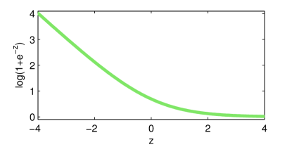
Because Equation (220) is convex in (it is the composition of the convex logistic loss function with a linear function of ), we can optimize it efficiently using projected gradient descent, where we alternate taking gradient steps and projecting on the constraint . The gradient is given by
| (221) |
where is a vector with entries
| (222) |
Projection onto the simplex is achieved using standard algorithms (Bertsekas, 1999).
5.3.2 Data
We create datasets for three broad image search categories, using 8–12 hand-selected queries for each category. (See Table 6.) For each query, we retrieve the top 64 results from Google Image Search, restricting the search to JPEG files that pass the strictest level of Safe Search filtering. Of those 64 results, we eliminate any that are no longer available for download. On average this leaves us with 63.0 images per query, with a range of 59–64.
| cars | cities | dogs |
|---|---|---|
| chrysler | baltimore | beagle |
| ford | barcelona | bernese |
| honda | london | blue heeler |
| mercedes | los angeles | cocker spaniel |
| mitsubishi | miami | collie |
| nissan | new york city | great dane |
| porsche | paris | labrador |
| toyota | philadelphia | pomeranian |
| san francisco | poodle | |
| shanghai | pug | |
| tokyo | schnauzer | |
| toronto | shih tzu |
We then use the downloaded images to generate 960 training instances for each category, spread evenly across the different queries. In order to compare -DPPs directly against baseline heuristic methods that do not model probabilities of full sets, we generate only instances where and differ by a single element. That is, the classification problem is effectively to choose which of two candidate images is a less redundant addition to a given partial result set :
| (223) |
In our experiments contains five images, so . We sample partial result sets using a -DPP with a SIFT-based kernel (details below) to encourage diversity. The candidates are then selected uniformly at random from the remaining images, except for 10% of instances that are reserved for measuring the performance of our human judges. For those instances, one of the candidates is a duplicate image chosen uniformly at random from the partial result set, making it the obviously more redundant choice. The other candidate is chosen as usual.
In order to decide which candidate actually results in the more diverse set, we collect human diversity judgments using Amazon’s Mechanical Turk. Annotators are drawn from the general pool of Turk workers, and are able to label as many instances as they wish. Annotators are paid $0.01 USD for each instance that they label. For practical reasons, we present the images to the annotators at reduced scale; the larger dimension of an image is always 250 pixels. The annotators are instructed to choose the candidate that they feel is “less similar” to the images in the partial result set. We do not offer any specific guidance on how to judge similarity, since dealing with uncertainty in human users is central to the task. The candidate images are presented in random order. Figure 15 shows a sample instance from each category.

Overall, we find that workers choose the correct image for 80.8% of the calibration instances (that is, they choose the one not belonging to the partial result set). This suggests only moderate levels of noise due to misunderstanding, inattention or robot workers. However, for non-calibration instances the task is inherently difficult and subjective. To keep noise in check, we have each instance labeled by five independent judges, and keep only those instances where four or more judges agree. In the end this leaves us with 408–482 labeled instances per category, or about half of the original instances.
5.3.3 Kernels
We define a set of 55 “expert” similarity kernels for the collected images, which form the building blocks of our combination model and baseline methods. Each kernel is the Gram matrix of some feature function ; that is, for images and . We therefore specify the kernels through the feature functions used to generate them. All of our feature functions are normalized so that for all ; this ensures that no image is a priori more likely than any other. Implicitly, thinking in terms of the decomposition in Section 3.1, we are assuming that all of the images in our set are equally relevant in order to isolate the modeling of diversity. This assumption is at least partly justified by the fact that our images come from actual Google searches, and are thus presumably relevant to the query.
We use the following feature functions, which derive from standard image processing and feature extraction methods:
-
•
Color (2 variants): Each pixel is assigned a coordinate in three-dimensional Lab color space. The colors are then sorted into axis-aligned bins, producing a histogram of either 8 or 64 dimensions.
-
•
SIFT (2 variants): The images are processed with the vlfeat toolbox to obtain sets of 128-dimensional SIFT descriptors (Lowe, 1999; Vedaldi and Fulkerson, 2008). The descriptors for a given category are combined, subsampled to a set of 25,000, and then clustered using -means into either 256 or 512 clusters. The feature vector for an image is the normalized histogram of the nearest clusters to the descriptors in the image.
-
•
GIST: The images are processed using code from Oliva and Torralba (2006) to yield 960-dimensional GIST feature vectors characterizing properties like “openness,” “roughness,” “naturalness,” and so on.
In addition to the five feature functions described above, we include another five that are identical but focus only on the center of the image, defined as the centered rectangle with dimensions half those of the original image. This gives our first ten kernels. We then create 45 pairwise combination kernels by concatenating every possible pair of the 10 basic feature vectors. This technique produces kernels that synthesize more than one source of information, offering greater flexibility.
Finally, we augment our kernels by adding a constant hyperparameter to each entry. acts a knob for controlling the overall preference for diversity; as increases, all images appear more similar, thus increasing repulsion. In our experiments, is chosen independently for each method and each category to optimize performance on the training set.
5.3.4 Methods
We test four different methods. Two use -DPPs, and two are derived from Maximum Marginal Relevance (MMR) (Carbonell and Goldstein, 1998). For each approach, we test both the single best expert kernel on the training data and a learned combination of kernels. All methods were tuned separately for each of the three query categories. On each run a random 25% of the labeled examples are reserved for testing, and the remaining 75% form the training set used for setting hyperparameters and training. Recall that is the five-image partial result set for instance , and let denote the set of two candidates images, where is the candidate preferred by the human judges.
Best -DPP
Given a single kernel , the -DPP prediction is
| (224) |
We select the kernel with the best zero-one accuracy on the training set, and apply it to the test set.
Mixture of -DPPs
We apply our learning method to the full set of 55 kernels, optimizing Equation (220) on the training set to obtain a 55-dimensional mixture vector . We set to minimize the zero-one training loss. We then take the learned and apply it to making predictions on the test set:
| (225) |
Best MMR
Recall that MMR is a standard, heuristic technique for generating diverse sets of search results. The idea is to build a set iteratively by adding on each round a result that maximizes a weighted combination of relevance (with respect to the query) and diversity, measured as the maximum similarity to any of the previously selected results. (See Section 4.2.1 for more details about MMR.) For our experiments, we assume relevance is uniform; hence we merely need to decide which of the two candidates has the smaller maximum similarity to the partial result set. Thus, for a given kernel , the MMR prediction is
| (226) |
As for the -DPP, we select the single best kernel on the training set, and apply it to the test set.
Mixture MMR
We can also attempt to learn a mixture of similarity kernels for MMR. We use the same training approach as for -DPPs, but replace the probability score with the negative cost
| (227) |
which is just the negative similarity of item to the set under the combined kernel metric. Significantly, this substitution makes the optimization non-smooth and non-convex, unlike the -DPP optimization. In practice this means that the global optimum is not easily found. However, even a local optimum may provide advantages over the single best kernel. In our experiments we use the local optimum found by projected gradient descent starting from the uniform kernel combination.
5.3.5 Results
Table 7 shows the mean zero-one accuracy of each method for each query category, averaged over 100 random train/test splits. Statistical significance is computed by bootstrapping. Regardless of whether we learn a mixture, -DPPs outperform MMR on two of the three categories, significant at 99% confidence. In all cases, the learned mixture of -DPPs achieves the best performance. Note that, because the decision being made for each instance is binary, 50% is equivalent to random performance. Thus the numbers in Table 7 suggest that this is a rather difficult task, a conclusion supported by the rates of noise exhibited by the human judges. However, the changes in performance due to learning and the use of -DPPs are more obviously significant when measured as improvements above this baseline level. For example, in the cars category our mixture of -DPPs performs 14.58 percentage points better than random, versus 9.59 points for MMR with a mixture of kernels. Figure 16 shows some actual samples drawn using the -DPP sampling algorithm.
| Best | Best | Mixture | Mixture | |
|---|---|---|---|---|
| Category | MMR | -DPP | MMR | -DPP |
| cars | 55.95 | 57.98 | 59.59 | 64.58 |
| cities | 56.48 | 56.31 | 60.99 | 61.29 |
| dogs | 56.23 | 57.70 | 57.39 | 59.84 |

Table 8 shows, for the -DPP mixture model, the kernels receiving the highest weights for each search category (on average over 100 train/test splits). Combined-feature kernels appear to be useful, and the three categories exhibit significant differences in what annotators deem diverse, as we might expect.
| color-8-center & sift-256 | (0.13) | |
| cars | color-8-center & sift-512 | (0.11) |
| color-8-center | (0.07) | |
| sift-512-center | (0.85) | |
| cities | gist | (0.08) |
| color-8-center & gist | (0.03) | |
| color-8-center | (0.39) | |
| dogs | color-8-center & sift-512 | (0.21) |
| color-8-center & sift-256 | (0.20) |
We can also return to our original motivation and try to measure how well each method “covers” the space of likely user intentions. Since we do not have access to real users who are searching for the queries in our dataset, we instead simulate them by imagining that each is looking for a particular target image drawn randomly from the images in our collection. For instance, given the query “philadelphia” we might draw a target image of the Love sculpture, and then evaluate each method on whether it selects an image of the Love sculpture, i.e., whether it satisfies that virtual user. More generally, we will simply record the maximum similarity of any image in the result set to the target image. We expect better methods to show higher similarity when averaged over a large number of such users.
| Single kernel | Uniform | MMR | |
|---|---|---|---|
| Category | (average) | mixture | mixture |
| cars | 57.58 | 68.31 | 58.15 |
| cities | 59.00 | 64.76 | 62.32 |
| dogs | 57.78 | 62.12 | 57.86 |
We consider only the mixture models here, since they perform best. For each virtual user, we sample a ten-image result set using the mixture -DPP, and select a second ten-image result set using the mixture MMR. For MMR, the first image is selected uniformly at random, since they are assumed to be uniformly relevant. Subsequent selections are deterministic. Given a target image drawn uniformly at random, we then compute similarities
| (228) |
for a particular similarity kernel . We report the fraction of the time that ; that is, the fraction of the time that our virtual user would be better served by the -DPP model. Because we have no gold standard kernel for measuring similarity, we try several possibilities, including all 55 expert kernels, a uniform combination of the expert kernels, and the combination learned by MMR. (Note that the mixture -DPP does not learn a kernel combination, hence there is no corresponding mixture to try here.) Table 9 shows the results, averaged across all of the virtual users (i.e., all the images in our collection). Even when using the mixture learned to optimize MMR itself, the -DPP does a better job of covering the space of possible user intentions. All results in Table 9 are significantly higher than 50% at 99% confidence.
6 Structured DPPs
We have seen in the preceding sections that DPPs offer polynomial-time inference and learning with respect to , the number of items in the ground set . This is important since DPPs model an exponential number of subsets , so naive algorithms would be intractable. And yet, we can imagine DPP applications for which even linear time is too slow. For example, suppose that after modeling the positions of basketball players, as proposed in the previous section, we wanted to take our analysis one step further. An obvious extension is to realize that a player does not simply occupy a single position, but instead moves around the court over time. Thus, we might want to model not just diverse sets of positions on the court, but diverse sets of paths around the court during a game. While we could reasonably discretize the possible court positions to a manageable number , the number of paths over, say, 100 time steps would be , making it almost certainly impossible to enumerate them all, let alone build an kernel matrix.
However, in this combinatorial setting we can take advantage of the fact that, even though there are exponentially many paths, they are structured; that is, every path is built from a small number of the same basic components. This kind of structure has frequently been exploited in machine learning, for example, to find the best translation of a sentence, or to compute the marginals of a Markov random field. In such cases structure allows us to factor computations over exponentially many possibilities in an efficient way. And yet, the situation for structured DPPs is even worse: when the number of items in is exponential, we are actually modeling a distribution over the doubly exponential number of subsets of an exponential . If there are possible paths, there are subsets of paths, and a DPP assigns a probability to every one. This poses an extreme computational challenge.
In order to develop efficient structured DPPs (SDPPs), we will therefore need to combine the dynamic programming techniques used for standard structured prediction with the algorithms that make DPP inference efficient. We will show how this can be done by applying the dual DPP representation from Section 3.3, which shares spectral properties with the kernel but is manageable in size, and the use of second-order message passing, where the usual sum-product or min-sum semiring is replaced with a special structure that computes quadratic quantities over a factor graph (Li and Eisner, 2009). In the end, we will demonstrate that it is possible to normalize and sample from an SDPP in polynomial time.
Structured DPPs open up a large variety of new possibilities for applications; they allow us to model diverse sets of essentially any structured objects. For instance, we could find not only the best translation but a diverse set of high-quality translations for a sentence, perhaps to aid a human translator. Or, we could study the distinct proteins coded by a gene under alternative RNA splicings, using the diversifying properties of DPPs to cover the large space of possibilities with a small representative set. Later, we will apply SDPPs to three real-world tasks: identifying multiple human poses in images, where there are combinatorially many possible poses, and we assume that the poses are diverse in that they tend not to overlap; identifying salient lines of research in a corpus of computer science publications, where the structures are citation chains of important papers, and we want to find a small number of chains that covers the major topic in the corpus; and building threads from news text, where the goal is to extract from a large corpus of articles the most significant news stories, and for each story present a sequence of articles covering the major developments of that story through time.
We begin by defining SDPPs and stating the structural assumptions that are necessary to make inference efficient; we then show how these assumptions give rise to polynomial-time algorithms using second order message passing. We discuss how sometimes even these polynomial algorithms can be too slow in practice, but demonstrate that by applying the technique of random projections (Section 3.4) we can dramatically speed up computation and reduce memory use while maintaining a close approximation to the original model (Kulesza and Taskar, 2010). Finally, we show how SDPPs can be applied to the experimental settings described above, yielding improved results compared with a variety of standard and heuristic baseline approaches.
6.1 Factorization
In Section 2.4 we saw that DPPs remain tractable on modern computers for up to around 10,000. This is no small feat, given that the number of subsets of 10,000 items is roughly the number of particles in the observable universe to the 40th power. Of course, this is not magic but simply a consequence of a certain type of structure; that is, we can perform inference with DPPs because the probabilities of these subsets are expressed as combinations of only a relatively small set of parameters. In order to make the jump now to ground sets that are exponentially large, we will need to make an similar assumption about the structure of itself. Thus, a structured DPP (SDPP) is a DPP in which the ground set is given implicitly by combinations of a set of parts. For instance, the parts could be positions on the court, and an element of a sequence of those positions. Or the parts could be rules of a context-free grammar, and then an element of might be a complete parse of a sentence. This assumption of structure will give us the algorithmic leverage we need to efficiently work with a distribution over a doubly exponential number of possibilities.
Because elements of are now structures, we will no longer think of ; instead, each element is a structure given by a sequence of parts , each of which takes a value from a finite set of possibilities. For example, if is the path of a basketball player, then is the number of time steps at which the player’s position is recorded, and is the player’s discretized position at time . We will use to denote the th structure in under an arbitrary ordering; thus , where . The parts of are denoted .
An immediate challenge is that the kernel , which has entries, can no longer be written down explicitly. We therefore define its entries using the quality/diversity decomposition presented in Section 3.1. Recall that this decomposition gives the entries of as follows:
| (229) |
where is a nonnegative measure of the quality of structure , and is a -dimensional vector of diversity features so that is a measure of the similarity between structures and . We cannot afford to specify and for every possible structure, but we can use the assumption that structures are built from parts to define a factorization, analogous to the factorization over cliques that gives rise to Markov random fields.
Specifically, we assume that the model decomposes over a set of factors , where a factor is a small subset of the parts of a structure. (Keeping the factors small will ensure that the model is tractable.) We denote by the collection of parts of that are included in factor ; then the factorization assumption is that the quality score decomposes multiplicatively over parts, and the diversity features decompose additively:
| (230) | ||||
| (231) |
We argue that these are quite natural factorizations. For instance, in our player tracking example we might have a positional factor for each time , allowing the quality model to prefer paths that go through certain high-traffic areas, and a transitional factor for each pair of times , allowing the quality model to enforce the smoothness of a path over time. More generally, if the parts correspond to cliques in a graph, then the quality scores can be given by a standard log-linear Markov random field (MRF), which defines a multiplicative distribution over structures that give labelings of the graph. Thus, while in Section 3.2 we compared DPPs and MRFs as alternative models for the same binary labeling problems, SDPPs can also be seen as an extension to MRFs, allowing us to take a model of individual structures and use it as a quality measure for modeling diverse sets of structures.
Diversity features, on the other hand, decompose additively, so we can think of them as global feature functions defined by summing local features, again as done in standard structured prediction. For example, could track the coarse-level position of a player at time , so that paths passing through similar positions at similar times are less likely to co-occur. Note that, in contrast to the unstructured case, we do not generally have , since there is no way to enforce such a constraint under the factorization in Equation (231). Instead, we simply set the factor features to have unit norm for all and all possible values of . This slightly biases the model towards structures that have the same (or similar) features at every factor, since such structures maximize . However, the effect of this bias seems to be minor in practice.
As for unstructured DPPs, the quality and diversity models combine to produce balanced, high-quality, diverse results. However, in the structured case the contribution of the diversity model can be especially significant due to the combinatorial nature of the items in . For instance, imagine taking a particular high-quality path and perturbing it slightly, say by shifting the position at each time step by a small random amount. This process results in a new and distinct path, but is unlikely to have a significant effect on the overall quality: the path remains smooth and goes through roughly the same positions. Of course, this is not unique to the structured case; we can have similar high-quality items in any DPP. What makes the problem especially serious here is that there is a combinatorial number of such slightly perturbed paths; the introduction of structure dramatically increases not only the number of items in , but also the number of subtle variations that we might want to suppress. Furthermore, factored distributions over structures are often very peaked due to the geometric combination of quality scores across many factors, so variations of the most likely structure can be much more probable than any real alternative. For these reasons independent samples from an MRF can often look nearly identical; a sample from an SDPP, on the other hand, is much more likely to contain a truly diverse set of structures.
6.1.1 Synthetic example: particle tracking
Before describing the technical details needed to make SDPPs computationally efficient, we first develop some intuition by studying the results of the model as applied to a synthetic motion tracking task, where the goal is to follow a collection of particles as they travel in a one-dimensional space over time. This is essentially a simplified version of our player tracking example, but with the motion restricted to a line. We will assume that a path has 50 parts, where each part is the particle’s position at time step discretized into one of 50 locations. The total number of possible trajectories in this setting is , and we will be modeling possible sets of trajectories. We define positional and transitional factors
| (232) |
While a real tracking problem would involve quality scores that depend on some observations—for example, measurements over time from a set of physical sensors, or perhaps a video feed from a basketball game—for simplicity we determine the quality of a trajectory here using only its starting position and a measure of smoothness over time. Specifically, we have
| (233) |
where the initial quality score is given by a smooth trimodal function with a primary mode at position 25 and secondary modes at positions 10 and 40, depicted by the blue curves on the left side of Figure 17, and the quality scores for all other positional factors are fixed to one and have no effect. The transition quality is the same at all time steps, and given by , where is the density function of the normal distribution; that is, the quality of a transition is maximized when the particle does not change location, and decreases as the particle moves further and further from its previous location. In essence, high quality paths start near the central position and move smoothly through time.
We want trajectories to be considered similar if they travel through similar positions, so we define a 50-dimensional diversity feature vector as follows:
| (234) | ||||
| (235) |
Intuitively, feature is activated when the trajectory passes near position , so trajectories passing through nearby positions will activate the same features and thus appear similar in the diversity model. Note that for simplicity, the time at which a particle reaches a given position has no effect on the diversity features. The diversity features for the transitional factors are zero and have no effect.
We use the quality and diversity models specified above to define our SDPP. In order to obtain good results for visualization, we scale the kernel so that the expected number of trajectories in a sample from the SDPP is five. We then apply the algorithms developed later to draw samples from the model. The first row of Figure 17 shows the results, and for comparison each corresponding panel on the second row shows an equal number of trajectories sampled independently, with probabilities proportional to their quality scores. As evident from the figure, trajectories sampled independently tend to cluster in the middle region due to the strong preference for this starting position. The SDPP samples, however, are more diverse, tending to cover more of the space while still respecting the quality scores—they are still smooth, and still tend to start near the center.
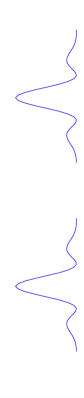
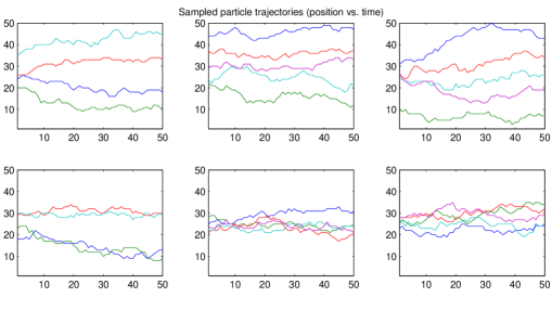
6.2 Second-order message passing
The central computational challenge for SDPPs is the fact that is exponentially large, making the usual inference algorithms intractable. However, we showed in Section 3.3 that DPP inference can be recast in terms of a smaller dual representation ; recall that, if is the matrix whose columns are given by , then and
| (236) | ||||
| (237) |
Of course, for the dual representation to be of any use we must be able to efficiently compute . If we think of as the factor potentials of a graphical model , then computing is equivalent to computing second moments of the diversity features under (up to normalization). Since the diversity features factor additively, is quadratic in the local diversity features . Thus, we could naively calculate by computing the pairwise marginals for all realizations of the factors and, by linearity of expectations, adding up their contributions:
| (238) |
where the proportionality is due to the normalizing constant of . However, this sum is quadratic in the number of factors and their possible realizations, and can therefore be expensive when structures are large.
Instead, we can substitute the factorization from Equation (231) into Equation (237) to obtain
| (239) |
It turns out that this expression is computable in linear time using a second-order message passing algorithm.
Second-order message passing was first introduced by Li and Eisner (2009). The main idea is to compute second-order statistics over a graphical model by using the standard belief propagation message passing algorithm, but with a special semiring in place of the usual sum-product or max-product. This substitution makes it possible to compute quantities of the form
| (240) |
where are nonnegative and and are arbitrary functions. Note that we can think of as defining a multiplicatively decomposed function
| (241) |
and and as defining corresponding additively decomposed functions and .
We begin by defining the notion of a factor graph, which provides the structure for all message passing algorithms. We then describe standard belief propagation on factor graphs, and show how it can be defined in a general way using semirings. Finally we demonstrate that belief propagation using the semiring proposed by Li and Eisner (2009) computes quantities of the form in Equation (240).
6.2.1 Factor graphs
Message passing operates on factor graphs. A factor graph is an undirected bipartite graph with two types of vertices: variable nodes and factor nodes. Variable nodes correspond to the parts of the structure being modeled; for the SDPP setup described above, a factor graph contains variable nodes, each associated with a distinct part . Similarly, each factor node corresponds to a distinct factor . Every edge in the graph connects a variable node to a factor node, and an edge exists between variable node and factor node if and only if . Thus, the factor graph encodes the relationships between parts and factors. Figure 18 shows an example factor graph for the tracking problem from Section 6.1.1.
It is obvious that the computation of Equation (240) cannot be efficient when factors are allowed to be arbitrary, since in the limit a factor could contain all parts and we could assign arbitrary values to every configuration . Thus we will assume that the degree of the factor nodes is bounded by a constant . (In Figure 18, as well as all of the experiments we run, we have .) Furthermore, message passing algorithms are efficient whenever the factor graph has low treewidth, or, roughly, when only small sets of nodes need to be merged to obtain a tree. Going forward we will assume that the factor graph is a tree, since any low-treewidth factor graph can be converted into an equivalent factor tree with bounded factors using the junction tree algorithm (Lauritzen and Spiegelhalter, 1988).
6.2.2 Belief propagation
We now describe the basic belief propagation algorithm, first introduced by Pearl (1982). Suppose each factor has an associated real-valued weight function , giving rise to the multiplicatively decomposed global weight function
| (242) |
Then the goal of belief propagation is to efficiently compute sums of over combinatorially large sets of structures .
We will refer to a structure as an assignment to the variable nodes of the factor graph, since it defines a value for every part. Likewise we can think of as an assignment to the variable nodes adjacent to , and as an assignment to a single variable node . We use the notation to indicate that is consistent with , in the sense that it assigns the same value to variable node . Finally, denote by the set of factors in which variable participates.
The belief propagation algorithm defines recursive message functions to be passed along edges of the factor graph; the formula for the message depends on whether it is traveling from a variable node to a factor node, or vice versa:
-
•
From a variable to a factor :
(243) -
•
From a factor to a variable :
(244)
Intuitively, an outgoing message summarizes all of the messages arriving at the source node, excluding the one coming from the target node. Messages from factor nodes additionally incorporate information about the local weight function.
Belief propagation passes these messages in two phases based on an arbitrary orientation of the factor tree. In the first phase, called the forward pass, messages are passed upwards from the leaves to the root. In the second phase, or backward pass, the messages are passed downward, from the root to the leaves. Upon completion of the second phase one message has been passed in each direction along every edge in the factor graph, and it is possible to prove using an inductive argument that, for every ,
| (245) |
If we think of the as potential functions, then Equation (245) gives the (unnormalized) marginal probability of the assignment under a Markov random field.
Note that the algorithm passes two messages per edge in the factor graph, and each message requires considering at most assignments, therefore its running time is . The sum on the right-hand side of Equation (245), however, is exponential in the number of parts. Thus belief propagation offers an efficient means of computing certain combinatorial quantities that would naively require exponential time.
6.2.3 Semirings
In fact, the belief propagation algorithm can be easily generalized to operate over an arbitrary semiring, thus allowing the same basic algorithm to perform a variety of useful computations. Recall that a semiring comprises a set of elements , an addition operator , a multiplication operator , an additive identity , and a multiplicative identity satisfying the following requirements for all :
-
•
Addition is associative and commutative, with identity :
(246) (247) (248) -
•
Multiplication is associative, with identity :
(249) (250) -
•
Multiplication distributes over addition:
(251) (252) -
•
is absorbing under multiplication:
(253)
Obviously these requirements are met when and multiplication and addition are the usual arithmetic operations; this is the standard sum-product semiring. We also have, for example, the max-product semiring, where , addition is given by the maximum operator with identity element 0, and multiplication is as before.
We can rewrite the messages defined by belief propagation in terms of these more general operations. For , we have
| (254) | ||||
| (255) |
As before, we can pass messages forward and then backward through the factor tree. Because the properties of semirings are sufficient to preserve the inductive argument, we then have the following analog of Equation (245):
| (256) |
We have seen that Equation (256) computes marginal probabilities under the sum-product semiring, but other semirings give rise to useful results as well. Under the max-product semiring, for instance, Equation (256) is the so-called max-marginal—the maximum unnormalized probability of any single assignment consistent with . In the next section we take this one step further, and show how a carefully designed semiring will allow us to sum second-order quantities across exponentially many structures .
6.2.4 Second-order semiring
Li and Eisner (2009) proposed the following second-order semiring over four-tuples :
| (257) | ||||
| (258) | ||||
| (259) | ||||
| (260) |
It is easy to verify that the semiring properties hold for these operations. Now, suppose that the weight function for a factor is given by
| (261) |
where , , and are as before. Then , and we can get some intuition about the multiplication operator by observing that the fourth component of is
| (262) | ||||
| (263) |
In other words, multiplication in the second-order semiring combines the values of multiplicatively and the values of and additively, leaving the result in the fourth component. It is not hard to extend this argument inductively and show that the fourth component of is given in general by
| (264) |
Thus, by Equation (256) and the definition of , belief propagation with the second-order semiring yields messages that satisfy
| (265) |
Note that multiplication and addition remain constant-time operations in the second-order semiring, thus belief propagation can still be performed in time linear in the number of factors. In the following section we will show that the dual representation , as well as related quantities needed to perform inference in SDPPs, takes the form of Equation (265); thus second-order message passing will be an important tool for efficient SDPP inference.
6.3 Inference
The factorization proposed in Equation (231) gives a concise definition of a structured DPP for an exponentially large ; remarkably, under suitable conditions it also gives rise to tractable algorithms for normalizing the SDPP, computing marginals, and sampling. The only restrictions necessary for efficiency are the ones we inherit from belief propagation: the factors must be of bounded size so that we can enumerate all of their possible configurations, and together they must form a low-treewidth graph on the parts of the structure. These are precisely the same conditions needed for efficient graphical model inference (Koller and Friedman, 2009), which is generalized by inference in SDPPs.
6.3.1 Computing
As we saw in Section 3.3, the dual representation is sufficient to normalize and marginalize an SDPP in time constant in . Recall from Equation (239) that the dual representation of an SDPP can be written as
| (266) |
which is of the form required to apply second-order message passing. Specifically, we can compute for each pair of diversity features the value of
| (267) |
by summing Equation (265) over the possible assignments , and then simply assemble the results into the matrix . Since there are unique entries in and message passing runs in time , computing in this fashion requires time.
We can make several practical optimizations to this algorithm, though they will not affect the asymptotic performance. First, we note that the full set of messages at any variable node is sufficient to compute Equation (267). Thus, during message passing we need only perform the forward pass; at that point, the messages at the root node are complete and we can obtain the quantity we need. This speeds up the algorithm by a factor of two. Second, rather than running message passing times, we can run it only once using a vectorized second-order semiring. This has no effect on the total number of operations, but can result in significantly faster performance due to vector optimizations in modern processors. The vectorized second-order semiring is over four-tuples where , , and , and uses the following operations:
| (268) | ||||
| (269) | ||||
| (270) | ||||
| (271) |
It is easy to verify that computations in this vectorized semiring are identical to those obtained by repeated use of the scalar semiring.
Given , we can now normalize and compute marginals for an SDPP using the formulas in Section 3.3; for instance
| (272) | ||||
| (273) |
where is an eigendecomposition of .
Part marginals
The introduction of structure offers an alternative type of marginal probability, this time not of structures but of single part assignments. More precisely, we can ask how many of the structures in a sample from the SDPP can be expected to make the assignment to part :
| (274) | ||||
| (275) |
The sum is exponential, but we can compute it efficiently using second-order message passing. We apply Equation (273) to get
| (276) | ||||
| (277) | ||||
| (278) |
The result is a sum of terms, each of which takes the form of Equation (265), and therefore is efficiently computable by message passing. The desired part marginal probability simply requires separate applications of belief propagation, one per eigenvector , for a total runtime of . (It is also possible to vectorize this computation and use a single run of belief propagation.) Note that if we require the marginal for only a single part , we can run just the forward pass if we root the factor tree at part node . However, by running both passes we obtain everything we need to compute the part marginals for any and ; the asymptotic time required to compute all part marginals is the same as the time required to compute just one.
6.3.2 Sampling
While the dual representation provides useful algorithms for normalization and marginals, the dual sampling algorithm is linear in ; for SDPPs, this is too slow to be useful. In order to make SDPP sampling practical, we need to be able to efficiently choose a structure according to the distribution
| (279) |
in the first line of the while loop in Algorithm 3. We can use the definition of to obtain
| (280) | ||||
| (281) |
Thus, the desired distribution has the familiar form of Equation (265). For instance, the marginal probability of part taking the assignment is given by
| (282) |
which we can compute with runs of belief propagation (or a single vectorized run), taking only time. More generally, the message-passing computation of these marginals offers an efficient algorithm for sampling individual full structures . We will first show a naive method based on iterated computation of conditional marginals, and then use it to derive a more efficient algorithm by integrating the sampling of parts into the message-passing process.
Single structure sampling
Returning to the factor graph used for belief propagation (see Section 6.2.1), we can force a part to take a certain assignment by adding a new singleton factor containing only , and setting its weight function to for and otherwise. (In practice, we do not need to actually create a new factor; we can simply set outgoing messages from variable to for all but the desired assignment .) It is easy to see that Equation (256) becomes
| (283) |
where the sum is now doubly constrained, since any assignment that is not consistent with introduces a into the product. If gives rise to a probability measure over structures , then Equation (283) can be seen as the unnormalized conditional marginal probability of the assignment given . For example, using the second-order semiring with and , we have
| (284) |
Summing these values for all and normalizing the result yields the conditional distribution of given fixed assignment under Equation (281). Going forward we will assume for simplicity that contains a single vector ; however, the general case is easily handled by maintaining messages in parallel, or by vectorizing the computation.
The observation that we can compute conditional probabilities with certain assignments held fixed gives rise to a naive algorithm for sampling a structure according to in Equation (281), shown in Algorithm 9. While polynomial, Algorithm 9 requires running belief propagation times, which might be prohibitively expensive for large structures. We can do better by weaving the sampling steps into a single run of belief propagation. We discuss first how this can be done for linear factor graphs, where the intuition is simpler, and then extend it to general factor trees.
Linear graphs
Suppose that the factor graph is a linear chain arranged from left to right. Each node in the graph has at most two neighbors—one to the left, and one to the right. Assume the belief propagation forward pass proceeds from left to right, and the backward pass from right to left. To send a message to the right, a node needs only to receive its message from the left. Conversely, to send a message to the left, only the message from the right is needed. Thus, the forward and backward passes can be performed independently.
Consider now the execution of Algorithm 9 on this factor graph. Assume the variable nodes are numbered in decreasing order from left to right, so the variable sampled in the first iteration is the rightmost variable node. Observe that on iteration , we do not actually need to run belief propagation to completion; we need only the messages incoming to variable node , since those suffice to compute the (conditional) marginals for part . To obtain those messages, we must compute all of the forward messages sent from the left of variable , and the backward messages from the right. Call this set of messages .
Note that is just a full, unconstrained forward pass, which can be computed in time . Now compare to . Between iteration and , the only change to is that variable , to the right of variable , has been assigned. Therefore the forward messages in , which come from the left, do not need to be recomputed, as they are a subset of the forward messages in . Likewise, the backward messages sent from the right of variable are unchanged, so they do not need to be recomputed. The only new messages in are those backward messages traveling from to . These can be computed, using and the sampled assignment , in constant time. See Figure 19 for an illustration of this process.
Thus, rather than restarting belief propagation on each loop of Algorithm 9, we have shown that we need only compute a small number of additional messages. In essence we have threaded the sampling of parts into the backward pass. After completing the forward pass, we sample ; we then compute the backward messages from to , sample , and so on. When the backward pass is complete, we sample the final assignment and are finished. Since the initial forward pass takes time and each of the subsequent iterations takes at most time, we can sample from over a linear graph in time.
Trees
The algorithm described above for linear graphs can be generalized to arbitrary factor trees. For standard graphical model sampling using the sum-product semiring, the generalization is straightforward—we can simply pass messages up to the root and then sample on the backward pass from the root to the leaves. However, for arbitrary semirings this is algorithm is incorrect, since an assignment to one node can affect the messages arriving at its siblings even when the parent’s assignment is fixed.
Let be the message function sent from node to node during a run of belief propagation where the assignments in have been held fixed. Imagine that we re-root the factor tree with as the root; then define to be the subtree rooted at (see Figure 20). Several useful observations follow.
Lemma 6.1.
If and are distinct neighbors of , then and are disjoint.
Proof.
The claim is immediate, since the underlying graph is a tree. ∎
Lemma 6.2.
can be computed given only the messages for all neighbors of and either the weight function (if is a factor node) or the assignment to in (if is a variable node and such an assignment exists).
Lemma 6.3.
depends only on the assignments in that give values to variables in .
Proof.
If is a leaf (that is, its only neighbor is ), the lemma holds trivially. If is not a leaf, then assume inductively that incoming messages , , depend only on assignments to variables in . By Lemma 6.2, the message depends only on those messages and (possibly) the assignment to in . Since and are subgraphs of , the claim follows. ∎
To sample a structure, we begin by initializing and setting messages for all neighbor pairs . This can be done in time via belief propagation.
Now we walk the graph, sampling assignments and updating the current messages as we go. Step from node to proceeds in three parts as follows:
-
1.
Check whether is a variable node without an assignment in . If so, sample an assignment using the current incoming messages , and set . Otherwise set .
- 2.
-
3.
Advance to node .
This simple algorithm has the following useful invariant.
Theorem 6.4.
Following step from to , for every neighbor of we have
| (285) |
Proof.
By design, the theorem holds at the outset of the walk. Suppose inductively that the claim is true for steps . Let be the most recent step prior to at which we visited , or if step was our first visit to . Since the graph is a tree, we know that between steps and the walk remained entirely within . Hence the only assignments in are to variables in . As a result, for all neighbors of we have by the inductive hypothesis, Lemma 6.1, and Lemma 6.3.
Theorem 285 guarantees that whenever we sample an assignment for the current variable node in the first part of step , we sample from the conditional marginal distribution . Therefore, we can sample a complete structure from the distribution if we walk the entire tree. This can be done, for example, by starting at the root and proceeding in depth-first order. Such a walk takes steps, and each step requires computing only a single message. Thus, allowing now for , we can sample a structure in time , a significant improvement over Algorithm 9. The procedure is summarized in Algorithm 10.
Algorithm 10 is the final piece of machinery needed to replicate the DPP sampling algorithm using the dual representation. The full SDPP sampling process is given in Algorithm 11 and runs in time , where is the number of eigenvectors selected in the first loop. As in standard DPP sampling, the asymptotically most expensive operation is the orthonormalization; here we require time to compute each of the dot products.
6.4 Experiments: pose estimation
To demonstrate that SDPPs effectively model characteristics of real-world data, we apply them to a multiple-person pose estimation task (Kulesza and Taskar, 2010). Our input will be a still image depicting multiple people, and our goal is to simultaneously identify the poses—the positions of the torsos, heads, and left and right arms—of all the people in the image. A pose is therefore a structure with four parts, in this case literally body parts. To form a complete structure, each part is assigned a position/orientation pair . Our quality model will be based on “part detectors” trained to estimate the likelihood of a particular body part at a particular location and orientation; thus we will focus on identifying poses that correspond well to the image itself. Our similarity model, on the other hand, will focus on the location of a pose within the image. Since the part detectors often have uncertainty about the precise location of a part, there may be many variations of a single pose that outscore the poses of all the other, less detectable people. An independent model would thus be likely to choose many similar poses. By encouraging the model to choose a spatially diverse set of poses, we hope to improve the chance that the model predicts a single pose for each person.
Our dataset consists of 73 still frames taken from various TV shows, each approximately 720 by 540 pixels in size (Sapp et al., 2010)333The images and code were obtained from http://www.vision.grasp.upenn.edu/video. As much as possible, the selected frames contain three or more people at similar scale, all facing the camera and without serious occlusions. Sample images from the dataset are shown in Figure 22. Each person in each image is annotated by hand; each of the four parts (head, torso, right arm, and left arm) is labeled with the pixel location of a reference point (e.g., the shoulder) and an orientation selected from among 24 discretized angles.
6.4.1 Factorized model
There are approximately 75,000 possible values for each part, so there are about possible poses, and thus we cannot reasonably use a standard DPP for this problem. Instead, we build a factorized SDPP. Our factors are given by the standard pictorial structure model (Felzenszwalb and Huttenlocher, 2005; Fischler and Elschlager, 1973), treating each pose as a two-level tree with the torso as the root and the head and arms as leaves. Each node (body part) has a singleton factor, and each edge has a corresponding pairwise factor.
Our quality function derives from the model proposed by Sapp et al. (2010), and is given by
| (286) |
where is the set of edges in the part tree, is a scale parameter that will control the expected number of poses in an SDPP sample, and is a sharpness parameter that controls the dynamic range of the quality scores. We set the values of the hyperparameters and using a held-out training set, as discussed below. The per-part quality scores are provided by the customized part detectors trained by Sapp et al. (2010) on similar images; they assign a value to every proposed location and orientation of part . The pairwise quality scores are defined according to a Gaussian “spring” that encourages, for example, the left arm to begin near the left shoulder of the torso. Full details of the model are provided in Sapp et al. (2010).
In order to encourage the model not to choose overlapping poses, our diversity features reflect the locations of the constituent parts:
| (287) |
where each . There are no diversity features on the edge factors. The local features are based on a grid of reference points spaced evenly across the image; the th feature is
| (288) |
Here is again the standard normal density function, and is the Euclidean distance between the position of part (ignoring orientation) and the reference point . Poses that occupy the same part of the image will be near the same reference points, and thus their feature vectors will be more closely aligned. The parameter controls the width of the kernel; larger values of make poses at a given distance appear more similar We set on a held-out training set.
6.4.2 Methods
We compare samples from the SDPP defined above to those from two baseline methods. The first, which we call the independent model, draws poses independently according to the distribution obtained by normalizing the quality scores, which is essentially the graphical model used by Sapp et al. (2010). For this model the number of poses to be sampled must be supplied by the user, so to create a level playing field we choose the number of poses in an SDPP sample . Since this approach does not incorporate a notion of diversity (or any correlations between selected poses whatsoever), we expect that we will frequently see multiple poses that correspond to the same person.
The second baseline is a simple non-maximum suppression model (Canny, 1986), which incorporates a heuristic for encouraging diversity. The first pose is drawn from the normalized quality model in the same manner as for the independent method. Subsequent poses, however, are constrained so that they cannot overlap with the previously selected poses, but otherwise drawn according to the quality model. We consider poses overlapping if they cover any of the same pixels when rendered. Again, the number of poses must be provided as an argument, so we use the number of poses from a sample of the SDPP. While the non-max approach can no longer generate multiple poses in the same location, it achieves this using a hard, heuristic constraint. Thus, we might expect to perform poorly when multiple people actually do overlap in the image, for example if one stands behind the other.
The SDPP, on the other hand, generates samples that prefer, but do not require poses to be spatially diverse. That is, strong visual information in the image can override our prior assumptions about the separation of distinct poses. We split our data randomly into a training set of 13 images and a test set of 60 images. Using the training set, we select values for , , and that optimize overall score at radius 100 (see below), as well as distinct optimal values of for the baselines. ( and are irrelevant for the baselines.) We then use each model to sample 10 sets of poses for each test image, for a total of 600 samples per model.
6.4.3 Results
For each sample from each of the three tested methods, we compute measures of precision and recall as well as an score. In our tests, precision is measured as the fraction of predicted parts for which both endpoints are within a given radius of the endpoints of an expert-labeled part of the same type (head, left arm, and so on). We report results across a range of radii. Correspondingly, recall is the fraction of expert-labeled parts with endpoints within a given radius of a predicted part of the same type. Since the SDPP model encourages diversity, we expect to see improvements in recall at the expense of precision, compared to the independent model. score is the harmonic mean of precision and recall. We compute all metrics separately for each sample, and then average the results across samples and images in the test set.
The results are shown in Figure 21a. At tight tolerances, when the radius of acceptance is small, the SDPP performs comparably to the independent and non-max samples, perhaps because the quality scores are simply unreliable at this resolution, thus diversity has little effect. As the radius increases, however, the SDPP obtains better results, significantly outperforming both baselines. Figure 21b shows the curves for just the arm parts, which tend to be more difficult to locate accurately and exhibit greater variance in orientation. Figure 21c shows the precision/recall obtained by each model. As expected, the SDPP model achieves its improved score by increasing recall at the cost of precision.
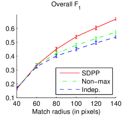
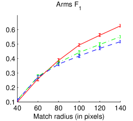
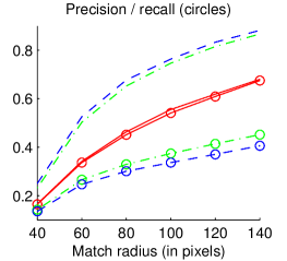
For illustration, we show the SDPP sampling process for some sample images from the test set in Figure 22. The SDPP part marginals are visualized as a “cloud”, where brighter colors correspond to higher probability. From left to right, we can see how the marginals change as poses are selected during the main loop of Algorithm 11. As we saw for simple synthetic examples in Figure 8a, the SDPP discounts but does not entirely preclude poses that are similar to those already selected.


6.5 Random projections for SDPPs
It is quite remarkable that we can perform polynomial-time inference for SDPPs given their extreme combinatorial nature. Even so, in some cases the algorithms presented in Section 6.3 may not be fast enough. Eigendecomposing the dual representation , for instance, requires time, while normalization, marginalization, and sampling, even when an eigendecomposition has been precomputed, scale quadratically in , both in terms of time and memory. In practice, this limits us to relatively low-dimensional diversity features ; for example, in our pose estimation experiments we built from a fairly coarse grid of 32 points mainly for reasons of efficiency. As we move to textual data, this will become an even bigger problem, since there is no natural low-dimensional analog for feature vectors based on, say, word occurrences. In the following section we will see data where natural vectors have dimension 30,000; without dimensionality reduction, storing even a single belief propagation message would require over 200 terabytes of memory.
To address this problem, we will make use of the random projection technique described in Section 3.4, reducing the dimension of the diversity features without sacrificing the accuracy of the model. Because Theorem 3.3 depends on a cardinality condition, we will focus on -SDPPs. As described in Section 5, a -DPP is simply a DPP conditioned on the cardinality of the modeled subset :
| (289) |
where denotes the matrix formed from columns for . When and factor over parts of a structure, as in Section 6.1, we will refer to this distribution as a -SDPP. We note in passing that the algorithms for normalization and sampling in Section 5 apply equally well to -SDPPs, since they depend mainly on the eigenvalues of , which we can obtain from .
Recall that Theorem 3.3 requires projection dimension
| (290) |
In the structured setting, , thus must be logarithmic in the number of labels and linear in the number of parts. Under this condition, we have, with probability at least ,
| (291) |
where is the projected -SDPP.
6.5.1 Toy example: geographical paths
In order to empirically study the effects of random projections, we test them on a simple toy application where is small enough that the exact model is tractable. The goal is to identify diverse, high-quality sets of travel routes between U.S. cities, where diversity is with respect to geographical location, and quality is optimized by short paths visiting the most populous or most touristy cities. Such sets of paths could be used, for example, by a politician to plan campaign routes, or by a traveler organizing a series of vacations.
We model the problem as a -SDPP over path structures having parts, where each part is a stop along the path and can take any of city values. The quality and diversity functions are factored, with a singleton factor for every individual stop and pairwise factors for consecutive pairs of stops. The quality of a singleton factor is based on the Google hit count for the assigned city, so that paths stopping in popular cities are preferred. The quality of a pair of consecutive stops is based on the distance between the assigned cities, so that short paths are preferred. In order to disallow paths that travel back and forth between the same cities, we augment the stop assignments to include arrival direction, and assign a quality score of zero to paths that return in the direction from which they came. The diversity features are only defined on the singleton factors; for a given city assignment , is just the vector of inverse distances between and all of the 200 cities. As a result, paths passing through the same or nearby cities appear similar, and the model prefers paths that travel through different regions of the country. We have .
Figure 23 shows sets of paths sampled from the -SDPP for various values of . For , the model tends to choose one path along the east coast and another along the west coast. As increases, a variety of configurations emerge; however, they continue to emphasize popular cities and the different paths remain geographically diverse.
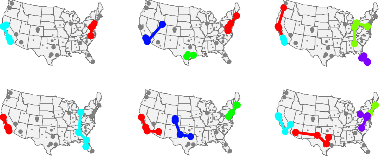
We can now investigate the effects of random projections on this model. Figure 24 shows the variational distance between the original model and the projected model (estimated by sampling), as well as the memory required to sample a set of paths for a variety of projection dimensions . As predicted by Theorem 3.3, only a relatively small number of projection dimensions are needed to obtain a close approximation to the original model. Past , the rate of improvement due to increased dimension falls off dramatically; meanwhile, the required memory and running time start to become significant. Figure 24 suggests that aggressive use of random projections, like those we employ in the following section, is not only theoretically but also empirically justified.
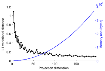
6.6 Experiments: threading graphs
In this section we put together many of the techniques introduced in this paper in order to complete a novel task that we refer to as graph threading (Gillenwater et al., 2012). The goal is to extract from a large directed graph a set of diverse, salient threads, or singly-connected chains of nodes. Depending on the construction of the graph, such threads can have various semantics. For example, given a corpus of academic literature, high-quality threads in the citation graph might correspond to chronological chains of important papers, each building on the work of the last. Thus, graph threading could be used to identify a set of significant lines of research. Or, given a collection of news articles from a certain time period, where each article is a node connected to previous, related articles, we might want to display the most significant news stories from that period, and for each story provide a thread that contains a timeline of its major events. We experiment on data from these two domains in the following sections. Other possibilities might include discovering trends on social media sites, for example, where users can post image or video responses to each other, or mining blog entries for important conversations through trackback links. Figure 25 gives an overview of the graph threading task for document collections.
Generally speaking, graph threading offers a means of gleaning insights from collections of interrelated objects—for instance, people, documents, images, events, locations, and so on—that are too large and noisy for manual examination. In contrast to tools like search, which require the user to specify a query based on prior knowledge, a set of threads provides an immediate, concise, high-level summary of the collection, not just identifying a set of important objects but also conveying the relationships between them. As the availability of such datasets continues to grow, this kind of automated analysis will be key in helping us to efficiently and effectively navigate and understand the information they contain.
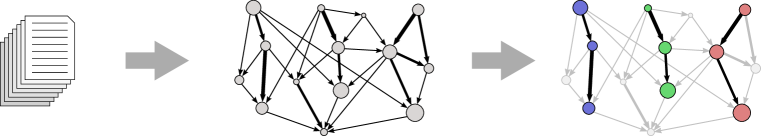
6.6.1 Related work
Research from to the Topic Detection and Tracking (TDT) program (Wayne, 2000) has led to useful methods for tasks like link detection, topic detection, and topic tracking that can be seen as subroutines for graph threading on text collections. Graph threading with -SDPPs, however, addresses these tasks jointly, using a global probabilistic model with a tractable inference algorithm.
Other work in the topic tracking literature has addressed related tasks (Mei and Zhai, 2005; Blei and Lafferty, 2006; Leskovec et al., 2009). In particular, Blei and Lafferty (2006) proposed dynamic topic models (DTMs), which, given a division of text documents into time slices, attempt to fit a generative model where topics evolve over time, and documents are drawn from the topics available at the time slice during which they were published. The evolving topics found by a DTM can be seen as threads of a sort, but in contrast to graph threading they are not composed of actual items in the dataset (in this case, documents). In Section 6.6.4 we will return to this distinction when we compare -SDPP threading to a DTM baseline.
The information retrieval community has produced other methods for extracting temporal information from document collections. Swan and Jensen (2000) proposed a system for finding temporally clustered named entities in news text and presenting them on a timeline. Allan et al. (2001) introduced the task of temporal summarization, which takes as input a stream of news articles related to a particular topic, and then seeks to extract sentences describing important events as they occur. Yan et al. (2011) evaluated methods for choosing sentences from temporally clustered documents that are relevant to a query. In contrast, graph threading seeks not to extract grouped entities or sentences, but instead to organize a subset of the objects (documents) themselves into threads, with topic identification as a side effect.
Some prior work has also focused more directly on threading. Shahaf and Guestrin (2010) and Chieu and Lee (2004) proposed methods for selecting individual threads, while Shahaf et al. (2012) recently proposed metro maps as alternative structured representations of related news stories. Metro maps are effectively sets of non-chronological threads that are encouraged to intersect and, in doing so, generate a map of events and topics. However, these approaches assume some prior knowledge about content. Shahaf and Guestrin (2010), for example, assume the thread endpoints are specified, and Chieu and Lee (2004) require a set of query words. Likewise, because they build metro maps individually, Shahaf et al. (2012) implicitly assume that the collection is filtered to a single topic, perhaps from a user query. These inputs make it possible to quickly pare down the document graph. In contrast, we will apply graph threading to very large graphs, and consider all possible threads.
6.6.2 Setup
In order to be as useful as possible, the threads we extract from a data graph need to be both high quality, reflecting the most important parts of the collection, and diverse, so that they cover distinct aspects of the data. In addition, we would like to be able to directly control both the length and the number of threads that we return, since different contexts might necessitate different settings. Finally, to be practical our method must be efficient in both time and memory use. -SDPPs with random projections allow us to simultaneously achieve all of these goals.
Given a directed graph on vertices with edge set and a real-valued weight function on nodes and edges, define the weight of a thread by
| (292) |
We can use to define a simple log-linear quality model for our -SDPP:
| (293) | ||||
| (294) |
where is a hyperparameter controlling the dynamic range of the quality scores. We fix the value of on a validation set in our experiments.
Likewise, let be a feature function from nodes in the graph to ; then the diversity feature function on threads is
| (295) |
In some cases it might also be convenient to have diversity features on edges of the graph as well as nodes. If so, they can be accommodated without much difficulty; however, for simplicity we proceed with the setup above.
We assume that , , and the projection dimension are provided; the first two depend on application context, and the third, as discussed in Section 6.5, is a tradeoff between computational efficiency and faithfulness to the original model. To generate diverse thread samples, we first project the diversity features by a random matrix whose entries are drawn independently and identically from . We then apply second-order message passing to compute the dual representation , as in Section 6.3.1. After eigendecomposing , which is only due to the projection, we can run the first phase of the -DPP sampling algorithm from Section 5.2.2 to choose a set of eigenvectors, and finally complete the SDPP sampling algorithm in Section 6.3.2 to obtain a set of threads . We now apply this model to two datasets; one is a citation graph of computer science papers, and the other is a large corpus of news text.
6.6.3 Academic citation data
The Cora dataset comprises a large collection of approximately 200,000 academic papers on computer science topics, including citation information (McCallum et al., 2000). We construct a directed graph with papers as nodes and citations as edges, and then remove papers with missing metadata or zero outgoing citations, leaving us with 28,155 papers. The average out-degree is citations per paper, and % of the total possible edges are present in the graph.
To obtain useful threads, we set edge weights to reflect the degree of textual similarity between the citing and the cited paper, and node weights to correspond with a measure of paper “importance”. Specifically, the weight of edge is given by the cosine similarity metric, which for two documents and is the dot product of their normalized tf-idf vectors, as defined in Section 4.2.1:
| (296) |
Here is a subset of the words found in the documents. We select by filtering according to document frequency; that is, we remove words that are too common, appearing in more than 10% of papers, or too rare, appearing in only one paper. After filtering, there are 50,912 unique words.
The node weights are given by the LexRank score of each paper (Erkan and Radev, 2004). The LexRank score is the stationary distribution of the thresholded, binarized, row-normalized matrix of cosine similarities, plus a damping term, which we fix to . LexRank is a measure of centrality, so papers that are closely related to many other papers will receive a higher score.
Finally, we design the diversity feature function to encourage topical diversity. Here we apply cosine similarity again, representing a document by the 1,000 documents to which it is most similar. This results in binary of dimension with exactly 1,000 non-zeros; implies that is one of the 1,000 most similar documents to . Correspondingly, the dot product between the diversity features of two documents is proportional to the fraction of top-1,000 documents they have in common. In order to make -SDPP inference efficient, we project down to dimensions.
Figure 26 illustrates the behavior of the model when we set and . Samples from the model, like the one presented in the figure, not only offer some immediate intuition about the types of papers contained in the collection, but also, upon examining individual threads, provide a succinct illustration of the content and development of each area. Furthermore, the sampled threads cover distinct topics, standing apart visually in Figure 26 and exhibiting diverse salient terms.
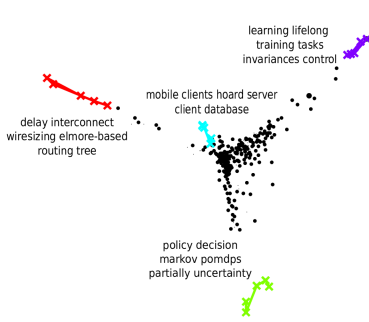
Thread: learning lifelong training tasks invariances control
1.
Locally Weighted Learning for Control
2.
Discovering Structure in Multiple Learning Tasks: The TC
Algorithm
3.
Learning One More Thing
4.
Explanation Based Learning for Mobile Robot Perception
5.
Learning Analytically and Inductively
Thread: mobile clients hoard server client database
1.
A Database Architecture for Handling Mobile Clients
2.
An Architecture for Mobile Databases
3.
Database Server Organization for Handling Mobile Clients
4.
Mobile Wireless Computing: Solutions and Challenges in
Data Management
5.
Energy Efficient Query Optimization
6.6.4 News articles
Our news dataset comprises over 200,000 articles from the New York Times, collected from 2005-2007 as part of the English Gigaword corpus (Graff and Cieri, 2009). We split the articles into six groups, with six months’ worth of articles in each group. Because the corpus contains a significant amount of noise in the form of articles that are short snippets, lists of numbers, and so on, we filter the results by discarding articles more than two standard deviations longer than the mean article, articles less than 400 words, and articles whose fraction of non-alphabetic words is more than two standard deviations above the mean. On average, for each six-month period we are left with 34,504 articles.
For each time period, we generate a graph with articles as nodes. As for the citations dataset, we use cosine similarity to define edge weights. The subset of words used to compute cosine similarity contains all words that appear in at least 20 articles and at most 15% of the articles. Across the six time periods, this results in an average of 36,356 unique words. We include in our graph only those edges with cosine similarity of at least 0.1; furthermore, we require that edges go forward in time to enforce the chronological ordering of threads. The resulting graphs have an average of % of the total possible edges, and an average degree of 107. As before, we use LexRank for node weights, and the top-1000 similar documents to define a binary feature function . We add a constant feature to , which controls the overall degree of repulsion; large values of make all documents more similar to one another. We set and the quality model hyperparameters to maximize a cosine similarity evaluation metric (see Section 6.6.4), using the data from the first half of 2005 as a development set. Finally, we randomly project the diversity features from to dimensions. For all of the following experiments, we use and . All evaluation metrics we report are averaged over random samples from the model.
Graph visualizations
In order to convey the scale and content of the graphs built from news data, we provide some high-resolution renderings. Figure 27 shows the graph neighborhood of a single article node from our development set. Each node represents an article and is annotated with the corresponding headline; the size of each node reflects its weight, as does the thickness of an edge. The horizontal position of a node corresponds to the time at which the article was published, from left to right; the vertical positions are optimized for readability. In the digital version of this paper, Figure 27 can be zoomed in order to read the headlines; in hardcopy, however, it is likely to be illegible. As an alternative, an online, zoomable version of the figure is available at http://zoom.it/GUCR.
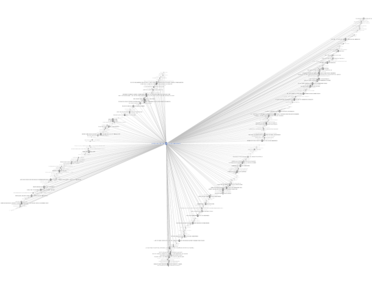
Visualizing the entire graph is quite challenging since it contains tens of thousands of nodes and millions of edges; placing such a figure in the paper would be impractical since the computational demands of rendering it and the zooming depth required to explore it would exceed the abilities of modern document viewers. Instead, we provide an online, zoomable version based upon a high-resolution (540 megapixel) rendering, available at http://zoom.it/jOKV. Even at this level of detail, only 1% of the edges are displayed; otherwise they become visually indistinct. As in Figure 27, each node represents an article and is sized according to its weight and overlaid with its headline. The horizontal position corresponds to time, ranging from January 2005 (on the left) to June 2005 (on the right). The vertical positions are determined by similarity to a set of threads sampled from the -SDPP, which are rendered in color.
Baselines
We will compare the -SDPP model to two natural baselines.
-means baseline. A simple method for this task is to split each six-month period of articles into equal-sized time slices, and then apply -means clustering to each slice, using cosine similarity at the clustering metric. We can then select the most central article from each cluster to form the basis of a set of threads. The articles chosen from time slice are matched one-to-one with those from slice by computing the pairing that maximizes the average cosine similarity of the pairs—that is, the coherence of the threads. Repeating this process for all yields a set of threads of length , where no two threads will contain the same article. However, because clustering is performed independently for each time slice, it is likely that the threads will sometimes exhibit discontinuities when the articles chosen at successive time slices do not naturally align.
DTM baseline. A natural extension, then, is the dynamic topic model (DTM) of Blei and Lafferty (2006), which explicitly attempts to find topics that are smooth through time. We use publicly available code444http://code.google.com/p/princeton-statistical-learning/ to fit DTMs with the number of topics set to and with the data split into equal time slices. We set the hyperparameters to maximize the cosine similarity metric (see Section 6.6.4) on our development set. We then choose, for each topic at each time step, the document with the highest per-word probability of being generated by that topic. Documents from the same topic form a single thread.
Figure 28 shows some of the threads sampled randomly from the -SDPP for our development set, and Figure 29 shows the same for threads produced by the DTM baseline. An obvious distinction is that topic model threads always span nearly the entire time period, selecting one article per time slice as required by the form of the model, while the DPP can select threads covering only the relevant span. Furthermore, the headlines in the figures suggest that the -SDPP produces more tightly focused, narrative threads due to its use of the data graph, while the DTM threads, though topically related, tend not to describe a single continuous news story. This distinction, which results from the fact that topic models are not designed with threading in mind, and so do not take advantage of the explicit relation information given by the graph, means that -SDPP threads often form a significantly more coherent representation of the news collection.
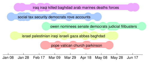
Thread: pope vatican church parkinson Feb 24: Parkinson’s Disease Increases Risks to Pope Feb 26: Pope’s Health Raises Questions About His Ability to Lead Mar 13: Pope Returns Home After 18 Days at Hospital Apr 01: Pope’s Condition Worsens as World Prepares for End of Papacy Apr 02: Pope, Though Gravely Ill, Utters Thanks for Prayers Apr 18: Europeans Fast Falling Away from Church Apr 20: In Developing World, Choice [of Pope] Met with Skepticism May 18: Pope Sends Message with Choice of Name
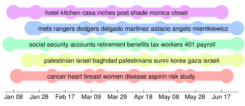
Thread: cancer heart breast women disease aspirin risk study Jan 11: Study Backs Meat, Colon Tumor Link Feb 07: Patients—and Many Doctors—Still Don’t Know How Often Women Get Heart Disease Mar 07: Aspirin Therapy Benefits Women, but Not in the Way It Aids Men Mar 16: Study Shows Radiation Therapy Doesn’t Increase Heart Disease Risk for Breast Cancer Patients Apr 11: Personal Health: Women Struggle for Parity of the Heart May 16: Black Women More Likely to Die from Breast Cancer May 24: Studies Bolster Diet, Exercise for Breast Cancer Patients Jun 21: Another Reason Fish is Good for You
Comparison to human summaries
We provide a quantitative evaluation of the threads generated by our baselines and sampled from the -SDPP by comparing them to a set of human-generated news summaries. The human summaries are not threaded; they are flat, approximately daily news summaries found in the Agence France-Presse portion of the Gigaword corpus, distinguished by their “multi” type tag. The summaries generally cover world news, which is only a subset of the contents of our dataset. Nonetheless, they allow us to provide an extrinsic evaluation for this novel task without generating gold standard timelines manually, which is a difficult task given the size of the corpus. We compute four metrics:
-
•
Cosine similarity. We concatenate the human summaries over each six-month period to obtain a target tf-idf vector, concatenate the set of threads to be evaluated to obtain a predicted tf-idf vector, and then compute the cosine similarity (in percent) between the target and predicted vectors. All hyperparameters are chosen to optimize this metric on a validation set.
- •
Table 10 shows the results of these comparisons, averaged over all six half-year intervals. Under each metric, the -SDPP produces threads that more closely resemble human summaries.
| ROUGE-1 | ROUGE-2 | ROUGE-SU4 | ||||||||
|---|---|---|---|---|---|---|---|---|---|---|
| System | Cos-sim | F | Prec / | Rec | F | Prec / | Rec | F | Prec / | Rec |
| -means | 29.9 | 16.5 | 17.3 / | 15.8 | 0.695 | 0.73 / | 0.67 | 3.76 | 3.94 / | 3.60 |
| DTM | 27.0 | 14.7 | 15.5 / | 14.0 | 0.750 | 0.81 / | 0.70 | 3.44 | 3.63 / | 3.28 |
| -SDPP | 33.2 | 17.2 | 17.7 / | 16.7 | 0.892 | 0.92 / | 0.87 | 3.98 | 4.11 / | 3.87 |
Mechanical Turk evaluation
| System | Rating | Interlopers |
|---|---|---|
| -means | 2.73 | 0.71 |
| DTM | 3.19 | 1.10 |
| -SDPP | 3.31 | 1.15 |
An important distinction between the baselines and the -SDPP is that the former are topic-oriented, choosing articles that relate to broad subject areas, while the -SDPP approach is story-oriented, chaining together articles with direct individual relationships. An example of this distinction can be seen in Figures 28 and 29.
To obtain a large-scale evaluation of this type of thread coherence, we employ Mechanical Turk, on online marketplace for inexpensively and efficiently completing tasks requiring human judgment. We asked Turkers to read the headlines and first few sentences of each article in a timeline and then rate the overall narrative coherence of the timeline on a scale of 1 (“the articles are totally unrelated”) to 5 (“the articles tell a single clear story”). Five separate Turkers rated each timeline. The average ratings are shown in the left column of Table 11; the -SDPP timelines are rated as significantly more coherent, while -means does poorly since it has no way to ensure that clusters are similar between time slices.
In addition, we asked Turkers to evaluate threads implicitly by performing a second task. (This also had the side benefit of ensuring that Turkers were engaged in the rating task and did not enter random decisions.) We displayed timelines into which two additional “interloper” articles selected at random had been inserted, and asked users to remove the two articles that they thought should be removed to improve the flow of the timeline. A screenshot of the task is provided in Figure 30. Intuitively, the true interlopers should be selected more often when the original timeline is coherent. The average number of interloper articles correctly identified is shown in the right column of Table 11.
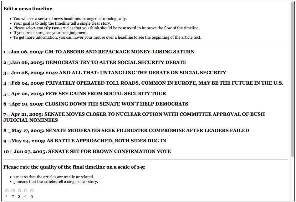
Runtime
Finally, assuming that tf-idf and feature values have been computed in advance (this process requires approximately 160 seconds), we report in Table 12 the time required to produce a set of threads on the development set. This measurement includes clustering for the -means baseline, model fitting for the DTM baseline, and random projections, computation of the covariance matrix, and sampling for the -SDPP. The tests were run on a machine with eight Intel Xeon E5450 cores and 32G of memory. Thanks to the use of random projections, the -SDPP is not only the most faithful to human news summaries, but also the fastest by a large margin.
| System | Runtime (s) | |
|---|---|---|
| -means | 625. | 63 |
| DTM | 19,433. | 80 |
| -SDPP | 252. | 38 |
7 Conclusion
We believe that DPPs offer exciting new possibilities for a wide range of practical applications. Unlike heuristic diversification techniques, DPPs provide coherent probabilistic semantics, and yet they do not suffer from the computational issues that plague existing models when negative correlations arise. Before concluding, we briefly mention two open technical questions, as well as some possible directions for future research.
7.1 Open question: concavity of entropy
The Shannon entropy of the DPP with marginal kernel is given by
| (297) |
Conjecture 7.1 (Lyons (2003)).
is concave in .
While numerical simulation strongly suggests that the conjecture is true, to our knowledge no proof currently exists.
7.2 Open question: higher-order sums
In order to calculate, for example, the Hellinger distance between a pair of DPPs, it would be useful to be able to compute quantities of the form
| (298) |
for . To our knowledge it is not currently known whether it is possible to compute these quantities efficiently.
7.3 Research directions
A variety of interesting machine learning questions remain for future research.
-
•
Would DPPs based on Hermitian or asymmetric kernels offer worthwhile modeling advantages?
-
•
Is there a simple characterization of the conditional independence relations encoded by a DPP?
-
•
Can we perform DPP inference under more complicated constraints on allowable sets? (For instance, if the items correspond to edges in a graph, we might only consider sets that comprise a valid matching.)
-
•
How can we learn the similarity kernel for a DPP (in addition to the quality model) from labeled training data?
-
•
How can we efficiently (perhaps approximately) work with SDPPs over loopy factor graphs?
-
•
Can SDPPs be used to diversify -best lists and improve reranking performance, for instance in parsing or machine translation?
References
- Abdelbar and Hedetniemi [1998] A.M. Abdelbar and S.M. Hedetniemi. Approximating maps for belief networks is np-hard and other theorems. Artificial Intelligence, 102(1):21–38, 1998.
- Allan et al. [2001] J. Allan, R. Gupta, and V. Khandelwal. Temporal Summaries of New Topics. In Proc. SIGIR, 2001.
- Baddeley and Van Lieshout [1995] AJ Baddeley and MNM Van Lieshout. Area-interaction point processes. Annals of the Institute of Statistical Mathematics, 47(4):601–619, 1995.
- Baker and Harwell [1996] F.B. Baker and M.R. Harwell. Computing elementary symmetric functions and their derivatives: A didactic. Applied Psychological Measurement, 20(2):169, 1996.
- Barvinok [1990] A.I. Barvinok. Computational complexity of immanents and representations of the full linear group. Functional Analysis and Its Applications, 24(2):144–145, 1990.
- Berthelsen and Møller [2006] K. Berthelsen and J. Møller. Bayesian analysis of markov point processes. Case studies in spatial point process modeling, pages 85–97, 2006.
- Bertsekas [1999] D. Bertsekas. Nonlinear Programming. Athena Scientific, Belmont, MA, 1999.
- Besag [1977] J. Besag. Some methods of statistical analysis for spatial data. Bulletin of the International Statistical Institute, 47(2):77–92, 1977.
- Besag and Green [1993] J. Besag and P.J. Green. Spatial statistics and bayesian computation. Journal of the Royal Statistical Society. Series B (Methodological), pages 25–37, 1993.
- Besag et al. [1982] J. Besag, R. Milne, and S. Zachary. Point process limits of lattice processes. Journal of Applied Probability, pages 210–216, 1982.
- Blei and Lafferty [2006] D.M. Blei and J.D. Lafferty. Dynamic topic models. In Proceedings of the 23rd international conference on Machine learning, pages 113–120. ACM, 2006.
- Borodin and Olshanski [2000] A. Borodin and G. Olshanski. Distributions on partitions, point processes, and the hypergeometric kernel. Communications in Mathematical Physics, 211(2):335–358, 2000.
- Borodin and Soshnikov [2003] A. Borodin and A. Soshnikov. Janossy densities. i. determinantal ensembles. Journal of statistical physics, 113(3):595–610, 2003.
- Borodin et al. [2010] A. Borodin, P. Diaconis, and J. Fulman. On adding a list of numbers (and other one-dependent determinantal processes). AMERICAN MATHEMATICAL SOCIETY, 47(4):639–670, 2010.
- Borodin [2009] Alexei Borodin. Determinantal point processes, 2009. URL http://arxiv.org/abs/0911.1153.
- Borodin and Rains [2005] Alexei Borodin and Eric Rains. Eynard–mehta theorem, schur process, and their pfaffian analogs. Journal of Statistical Physics, 121:291–317, 2005. ISSN 0022-4715. 10.1007/s10955-005-7583-z.
- Boros and Hammer [2002] E. Boros and P.L. Hammer. Pseudo-boolean optimization. Discrete Applied Mathematics, 123(1-3):155–225, 2002.
- Bratley and Fox [1988] P. Bratley and B.L. Fox. Algorithm 659: Implementing sobol’s quasirandom sequence generator. ACM Transactions on Mathematical Software (TOMS), 14(1):88–100, 1988.
- Brylinski and Brylinski [2003] J.L. Brylinski and R. Brylinski. Complexity and completeness of immanants. Arxiv preprint cs/0301024, 2003.
- Bürgisser [2000] P. Bürgisser. The computational complexity of immanants. SIAM Journal on Computing, 30:1023, 2000.
- Burton and Pemantle [1993] R. Burton and R. Pemantle. Local characteristics, entropy and limit theorems for spanning trees and domino tilings via transfer-impedances. The Annals of Probability, pages 1329–1371, 1993.
- Canny [1986] J. Canny. A computational approach to edge detection. Pattern Analysis and Machine Intelligence, IEEE Transactions on, 6:679–698, 1986.
- Carbonell and Goldstein [1998] J. Carbonell and J. Goldstein. The use of MMR, diversity-based reranking for reordering documents and producing summaries. In Proc. SIGIR, 1998.
- Cayley [1843] A. Cayley. On the theory of determinants. Transaction of the Cambridge Philosophical Society, 8(1843):1–16, 1843.
- Chekuri et al. [2011] C. Chekuri, J. Vondrák, and R. Zenklusen. Submodular function maximization via the multilinear relaxation and contention resolution schemes. Arxiv preprint arXiv:1105.4593, 2011.
- Chen and Karger [2006] H. Chen and D.R. Karger. Less is more: probabilistic models for retrieving fewer relevant documents. In Proce. SIGIR, pages 429–436, 2006.
- Chieu and Lee [2004] H. Chieu and Y. Lee. Query Based Event Extraction along a Timeline. In Proc. SIGIR, 2004.
- Çivril and Magdon-Ismail [2009] A. Çivril and M. Magdon-Ismail. On selecting a maximum volume sub-matrix of a matrix and related problems. Theoretical Computer Science, 410(47-49):4801–4811, 2009.
- Conroy et al. [2004] J.M. Conroy, J.D. Schlesinger, J. Goldstein, and D.P. O’leary. Left-brain/right-brain multi-document summarization. In Proceedings of the Document Understanding Conference (DUC 2004), 2004.
- Cooper [1990] G.F. Cooper. The computational complexity of probabilistic inference using bayesian belief networks. Artificial intelligence, 42(2-3):393–405, 1990.
- Dagum and Luby [1993] P. Dagum and M. Luby. Approximating probabilistic inference in bayesian belief networks is np-hard. Artificial intelligence, 60(1):141–153, 1993.
- Daley and Vere-Jones [2003] D.J. Daley and D. Vere-Jones. An introduction to the theory of point processes: volume I: elementary theory and methods. Springer, 2003.
- Daley and Vere-Jones [2008] D.J. Daley and D. Vere-Jones. An introduction to the theory of point processes: General theory and structure, volume 2. Springer Verlag, 2008.
- Dang [2005] H.T. Dang. Overview of DUC 2005. In Proce. DUC, 2005.
- Deshpande and Rademacher [2010] A. Deshpande and L. Rademacher. Efficient volume sampling for row/column subset selection. In 2010 IEEE 51st Annual Symposium on Foundations of Computer Science, pages 329–338. IEEE, 2010.
- Diaconis [2003] P. Diaconis. Patterns in eigenvalues: the 70th josiah willard gibbs lecture. BULLETIN-AMERICAN MATHEMATICAL SOCIETY, 40(2):155–178, 2003.
- Diaconis and Evans [2000] P. Diaconis and S.N. Evans. Immanants and finite point processes. Journal of Combinatorial Theory, Series A, 91(1-2):305–321, 2000.
- Diggle et al. [1987] P.J. Diggle, D.J. Gates, and A. Stibbard. A nonparametric estimator for pairwise-interaction point processes. Biometrika, 74(4):763–770, 1987.
- Diggle et al. [1994] P.J. Diggle, T. Fiksel, P. Grabarnik, Y. Ogata, D. Stoyan, and M. Tanemura. On parameter estimation for pairwise interaction point processes. International Statistical Review/Revue Internationale de Statistique, pages 99–117, 1994.
- Dyson [1962a] F.J. Dyson. Statistical theory of the energy levels of complex systems. i. Journal of Mathematical Physics, 3:140–156, 1962a.
- Dyson [1962b] F.J. Dyson. Statistical theory of the energy levels of complex systems. ii. Journal of Mathematical Physics, 3(157–165), 1962b.
- Dyson [1962c] F.J. Dyson. Statistical theory of the energy levels of complex systems. iii. Journal of Mathematical Physics, 3:166–175, 1962c.
- Erkan and Radev [2004] G. Erkan and D.R. Radev. LexRank: Graph-based lexical centrality as salience in text summarization. Journal of Artificial Intelligence Research, 22(1):457–479, 2004. ISSN 1076-9757.
- Evans and Gottlieb [2009] S.N. Evans and A. Gottlieb. Hyperdeterminantal point processes. Metrika, 69(2):85–99, 2009.
- Feder [1980] J. Feder. Random sequential adsorption. Journal of Theoretical Biology, 87(2):237–254, 1980.
- Feige [1998] U. Feige. A threshold of ln n for approximating set cover. Journal of the ACM (JACM), 45(4):634–652, 1998.
- Feige et al. [2007] U. Feige, V.S. Mirrokni, and J. Vondrak. Maximizing non-monotone submodular functions. In Foundations of Computer Science, 2007. FOCS’07. 48th Annual IEEE Symposium on, pages 461–471. IEEE, 2007.
- Feldman et al. [2011a] M. Feldman, J. Naor, and R. Schwartz. Nonmonotone submodular maximization via a structural continuous greedy algorithm. Automata, Languages and Programming, pages 342–353, 2011a.
- Feldman et al. [2011b] M. Feldman, J.S. Naor, and R. Schwartz. A unified continuous greedy algorithm for submodular maximization. In Foundations of Computer Science (FOCS), 2011 IEEE 52nd Annual Symposium on, pages 570–579. IEEE, 2011b.
- Felzenszwalb and Huttenlocher [2005] P.F. Felzenszwalb and D.P. Huttenlocher. Pictorial structures for object recognition. International Journal of Computer Vision, 61(1):55–79, 2005. ISSN 0920-5691.
- Finegold and Donnell [1979] L. Finegold and J.T. Donnell. Maximum density of random placing of membrane particles. Nature, 1979.
- Fischler and Elschlager [1973] MA Fischler and RA Elschlager. The representation and matching of pictorial structures. IEEE Transactions on Computers, 100(22), 1973.
- Fisher et al. [1978] M.L. Fisher, G.L. Nemhauser, and L.A. Wolsey. An analysis of approximations for maximizing submodular set functions—ii. Polyhedral combinatorics, pages 73–87, 1978.
- Gel’fand [1989] I.M. Gel’fand. Lectures on linear algebra. Dover, 1989. ISBN 0486660826.
- Genest et al. [2010] P.E. Genest, G. Lapalme, and M. Yousfi-Monod. Hextac: the creation of a manual extractive run. In Proceedings of the Second Text Analysis Conference, Gaithersburg, Maryland, USA: National Institute of Standards and Technology, 2010.
- Gharan and Vondrák [2011] S.O. Gharan and J. Vondrák. Submodular maximization by simulated annealing. In Proc. Soda, pages 1098–1116, 2011.
- Gillenwater et al. [2012] J. Gillenwater, A. Kulesza, and B. Taskar. Discovering diverse and salient threads in document collections. In Proceedings of the 2012 Conference on Empirical Methods in Machine Learning, 2012.
- Ginibre [1965] J. Ginibre. Statistical ensembles of complex, quaternion, and real matrices. Journal of Mathematical Physics, 6:440, 1965.
- Goel and Byrne [2000] V. Goel and W.J. Byrne. Minimum bayes-risk automatic speech recognition. Computer Speech & Language, 14(2):115–135, 2000.
- Graff and Cieri [2009] D. Graff and C. Cieri. English Gigaword, 2009.
- Grimmett [1973] G. R. Grimmett. A theorem about random fields. Bulletin of the London Mathematical Society, 5(13):81–84, 1973.
- Grone and Merris [1984] R. Grone and R. Merris. An algorithm for the second immanant. Math. Comp, 43:589–591, 1984.
- Häggström et al. [1999] O. Häggström, M.C.N.M. Van Lieshout, and J. Møller. Characterization results and markov chain monte carlo algorithms including exact simulation for some spatial point processes. Bernoulli, 5(4):641–658, 1999.
- Halton [1960] J.H. Halton. On the efficiency of certain quasi-random sequences of points in evaluating multi-dimensional integrals. Numerische Mathematik, 2(1):84–90, 1960.
- Hartmann [1985] W. Hartmann. On the complexity of immanants. Linear and Multilinear Algebra, 18(2):127–140, 1985.
- Hinrichsen et al. [1986] E.L. Hinrichsen, J. Feder, and T. Jøssang. Geometry of random sequential adsorption. Journal of statistical physics, 44(5):793–827, 1986.
- Hlawka [1961] E. Hlawka. Funktionen von beschränkter variatiou in der theorie der gleichverteilung. Annali di Matematica Pura ed Applicata, 54(1):325–333, 1961.
- Hough et al. [2006] J.B. Hough, M. Krishnapur, Y. Peres, and B. Virág. Determinantal processes and independence. Probability Surveys, 3:206–229, 2006.
- Huber and Wolpert [2009] M.L. Huber and R.L. Wolpert. Likelihood-based inference for matérn type-iii repulsive point processes. Advances in Applied Probability, 41(4):958–977, 2009.
- Ishikawa [2003] H. Ishikawa. Exact optimization for markov random fields with convex priors. Pattern Analysis and Machine Intelligence, IEEE Transactions on, 25(10):1333–1336, 2003.
- Jensen and Moller [1991] J.L. Jensen and J. Moller. Pseudolikelihood for exponential family models of spatial point processes. The Annals of Applied Probability, 1(3):445–461, 1991.
- Johansson [2002] K. Johansson. Non-intersecting paths, random tilings and random matrices. Probability theory and related fields, 123(2):225–280, 2002.
- Johansson [2004] K. Johansson. Determinantal processes with number variance saturation. Communications in mathematical physics, 252(1):111–148, 2004.
- Johansson [2005a] K. Johansson. The arctic circle boundary and the airy process. The annals of probability, 33(1):1–30, 2005a.
- Johansson [2005b] K. Johansson. Random matrices and determinantal processes. Arxiv preprint math-ph/0510038, 2005b.
- Johnson and Lindenstrauss [1984] W.B. Johnson and J. Lindenstrauss. Extensions of lipschitz mappings into a hilbert space. Contemporary mathematics, 26(189-206):1–1, 1984.
- Ko et al. [1995] C.W. Ko, J. Lee, and M. Queyranne. An exact algorithm for maximum entropy sampling. Operations Research, 43(4):684–691, 1995. ISSN 0030-364X.
- Koller and Friedman [2009] D. Koller and N. Friedman. Probabilistic Graphical Models: Principles and Techniques. The MIT Press, 2009.
- Kolmogorov and Zabih [2004] V. Kolmogorov and R. Zabih. What energy functions can be minimized via graph cuts? IEEE transactions on pattern analysis and machine intelligence, pages 147–159, 2004.
- Krause and Guestrin [2005] A. Krause and C. Guestrin. A note on the budgeted maximization of submodular functions. Technical Rep. No. CMU-CALD, 5:103, 2005.
- Kulesza and Pereira [2008] A. Kulesza and F. Pereira. Structured learning with approximate inference. Advances in neural information processing systems, 20:785–792, 2008.
- Kulesza and Taskar [2011a] A. Kulesza and B. Taskar. k-DPPs: fixed-size determinantal point processes. In Proceedings of the 28th International Conference on Machine Learning, 2011a.
- Kulesza and Taskar [2011b] A. Kulesza and B. Taskar. Learning determinantal point processes. In Proceedings of the 27th Conference on Uncertainty in Artificial Intelligence, 2011b.
- Kulesza and Taskar [2010] Alex Kulesza and Ben Taskar. Structured determinantal point processes. In Proc. Neural Information Processing Systems, 2010.
- Kulesza et al. [2012] Alex Kulesza, Jennifer Gillenwater, and Ben Taskar. Near-optimal map inference for determinantal point processes. In Proc. Neural Information Processing Systems, 2012.
- Kumar and Byrne [2002] S. Kumar and W. Byrne. Minimum bayes-risk word alignments of bilingual texts. In Proceedings of the ACL-02 conference on Empirical methods in natural language processing-Volume 10, pages 140–147. Association for Computational Linguistics, 2002.
- Kumar and Byrne [2004] S. Kumar and W. Byrne. Minimum bayes-risk decoding for statistical machine translation. In Proceedings of HLT-NAACL, pages 169–176, 2004.
- Lafferty et al. [2001] J.D. Lafferty, A. McCallum, and F.C.N. Pereira. Conditional random fields: Probabilistic models for segmenting and labeling sequence data. In Proceedings of the Eighteenth International Conference on Machine Learning, pages 282–289. Morgan Kaufmann Publishers Inc., 2001.
- Lauritzen and Spiegelhalter [1988] S.L. Lauritzen and D.J. Spiegelhalter. Local computations with probabilities on graphical structures and their application to expert systems. Journal of the Royal Statistical Society. Series B (Methodological), pages 157–224, 1988.
- Lee et al. [2009] J. Lee, V.S. Mirrokni, V. Nagarajan, and M. Sviridenko. Non-monotone submodular maximization under matroid and knapsack constraints. In Proceedings of the 41st annual ACM symposium on Theory of computing, pages 323–332. ACM, 2009.
- Leskovec et al. [2009] J. Leskovec, L. Backstrom, and J. Kleinberg. Meme-tracking and the Dynamics of the News Cycle. In Proc. KDD, 2009.
- Li and Eisner [2009] Z. Li and J. Eisner. First-and second-order expectation semirings with applications to minimum-risk training on translation forests. In Proc. EMNLP, 2009.
- Lin [2004] C.Y. Lin. Rouge: A package for automatic evaluation of summaries. In Proceedings of the workshop on text summarization branches out (WAS 2004), pages 25–26, 2004.
- Lin and Bilmes [2010] Hui Lin and Jeff Bilmes. Multi-document summarization via budgeted maximization of submodular functions. In Proc. NAACL/HLT, 2010.
- Lin and Bilmes [2012] Hui Lin and Jeff Bilmes. Learning mixtures of submodular shells with application to document summarization. In Uncertainty in Artificial Intelligence (UAI), Catalina Island, USA, July 2012. AUAI.
- Lowe [1999] D.G. Lowe. Object recognition from local scale-invariant features. In Proc. ICCV, 1999.
- Lyons [2003] R. Lyons. Determinantal probability measures. Publications Mathématiques de l’IHÉS, 98(1):167–212, 2003.
- Macchi [1975] O. Macchi. The coincidence approach to stochastic point processes. Advances in Applied Probability, 7(1):83–122, 1975.
- Magen and Zouzias [2008] A. Magen and A. Zouzias. Near optimal dimensionality reductions that preserve volumes. Approximation, Randomization and Combinatorial Optimization. Algorit hms and Techniques, pages 523–534, 2008.
- Matérn [1960] B. Matérn. Spatial variation. stochastic models and their application to some problems in forest surveys and other sampling investigations. Meddelanden fran statens Skogsforskningsinstitut, 49(5), 1960.
- Matérn [1986] B. Matérn. Spatial variation. Springer-Verlag, 1986.
- McCallum et al. [2000] A. McCallum, K. Nigam, J. Rennie, and K. Seymore. Automating the Construction of Internet Portals with Machine Learning. Information Retrieval Journal, 3:127–163, 2000.
- McCullagh and Møller [2006] P. McCullagh and J. Møller. The permanental process. Advances in applied probability, pages 873–888, 2006.
- Mehta and Gaudin [1960] M.L. Mehta and M. Gaudin. On the density of eigenvalues of a random matrix. Nuclear Physics, 18(0):420 – 427, 1960. ISSN 0029-5582. doi: 10.1016/0029-5582(60)90414-4. URL http://www.sciencedirect.com/science/article/pii/0029558260904144.
- Mei and Zhai [2005] W. Mei and C. Zhai. Discovering Evolutionary Theme Patterns From Text: An Exploration of T emporal Text Mining. In Proc. KDD, 2005.
- Møller and Waagepetersen [2004] J. Møller and R.P. Waagepetersen. Statistical inference and simulation for spatial point processes, volume 100. CRC Press, 2004.
- Møller and Waagepetersen [2007] J. Møller and R.P. Waagepetersen. Modern statistics for spatial point processes*. Scandinavian Journal of Statistics, 34(4):643–684, 2007.
- Møller et al. [2010] J. Møller, M.L. Huber, and R.L. Wolpert. Perfect simulation and moment properties for the matérn type iii process. Stochastic Processes and their Applications, 120(11):2142–2158, 2010.
- Murphy et al. [1999] K.P. Murphy, Y. Weiss, and M.I. Jordan. Loopy belief propagation for approximate inference: An empirical study. In Proceedings of the Fifteenth conference on Uncertainty in artificial intelligence, pages 467–475. Morgan Kaufmann Publishers Inc., 1999.
- Nemhauser et al. [1978] G.L. Nemhauser, L.A. Wolsey, and M.L. Fisher. An analysis of approximations for maximizing submodular set functions—i. Mathematical Programming, 14(1):265–294, 1978.
- Nenkova et al. [2006] Ani Nenkova, Lucy Vanderwende, and Kathleen McKeown. A compositional context sensitive multi-document summarizer: exploring the factors that influence summarization. In Proc. SIGIR, 2006.
- Niederreiter [1992] H. Niederreiter. Quasi-Monte Carlo Methods. Wiley Online Library, 1992.
- Nocedal [1980] J. Nocedal. Updating quasi-Newton matrices with limited storage. Mathematics of computation, 35(151):773–782, 1980.
- Ogata and Tanemura [1984] Y. Ogata and M. Tanemura. Likelihood analysis of spatial point patterns. Journal of the Royal Statistical Society. Series B (Methodological), pages 496–518, 1984.
- Ogata and Tanemura [1985] Y. Ogata and M. Tanemura. Estimation of interaction potentials of marked spatial point patterns through the maximum likelihood method. Biometrics, pages 421–433, 1985.
- Okounkov [2001] A. Okounkov. Infinite wedge and random partitions. Selecta Mathematica, New Series, 7(1):57–81, 2001.
- Okounkov and Reshetikhin [2003] A. Okounkov and N. Reshetikhin. Correlation function of schur process with application to local geometry of a random 3-dimensional young diagram. JOURNAL-AMERICAN MATHEMATICAL SOCIETY, 16(3):581–604, 2003.
- Oliva and Torralba [2006] A. Oliva and A. Torralba. Building the gist of a scene: The role of global image features in recognition. Progress in brain research, 155:23–36, 2006. ISSN 0079-6123.
- Pearl [1982] J. Pearl. Reverend bayes on inference engines: A distributed hierarchical approach. In Proceedings of the AAAI National Conference on AI, pages 133–136, 1982.
- Preston [1976] C.J. Preston. Random fields. Springer-Verlag New York, 1976.
- Radlinski et al. [2008] F. Radlinski, R. Kleinberg, and T. Joachims. Learning diverse rankings with multi-armed bandits. In Proc. ICML, 2008.
- Raman et al. [2012] K. Raman, P. Shivaswamy, and T. Joachims. Learning to diversify from implicit feedback. In WSDM Workshop on Diversity in Document Retrieval, 2012.
- Ramsden [1993] JJ Ramsden. Review of new experimental techniques for investigating random sequential adsorption. Journal of statistical physics, 73(5):853–877, 1993.
- Ripley [1991] B.D. Ripley. Statistical inference for spatial processes. Cambridge Univ Pr, 1991.
- Ripley and Kelly [1977] BD Ripley and FP Kelly. Markov point processes. Journal of the London Mathematical Society, 2(1):188, 1977.
- Sapp et al. [2010] Ben Sapp, Chris Jordan, and Ben Taskar. Adaptive pose priors for pictorial structures. In IEEE Computer Society Conference on Computer Vision and Pattern Recognition (CVPR’10), 2010.
- Schrijver [2000] A. Schrijver. A combinatorial algorithm minimizing submodular functions in strongly polynomial time. Journal of Combinatorial Theory, Series B, 80(2):346–355, 2000.
- Shahaf and Guestrin [2010] D. Shahaf and C. Guestrin. Connecting the Dots Between News Articles. In KDD, 2010.
- Shahaf et al. [2012] D. Shahaf, C. Guestrin, and E. Horvitz. Trains of Thought: Generating Information Maps. In Proc. WWW, 2012.
- Shimony [1994] S.E. Shimony. Finding maps for belief networks is np-hard. Artificial Intelligence, 68(2):399–410, 1994.
- Shirai and Takahashi [2000] T. Shirai and Y. Takahashi. Fermion process and fredholm determinant. In Proceedings of the second ISAAC Congress, volume 1, pages 15–23. Kluwer Academic Pub, 2000.
- Shirai and Takahashi [2003a] T. Shirai and Y. Takahashi. Random point fields associated with certain fredholm determinants i: fermion, poisson and boson point processes. Journal of Functional Analysis, 205(2):414–463, 2003a.
- Shirai and Takahashi [2003b] T. Shirai and Y. Takahashi. Random point fields associated with certain fredholm determinants ii: Fermion shifts and their ergodic and gibbs properties. The Annals of Probability, 31(3):1533–1564, 2003b.
- Sobol [1967] I.M. Sobol. On the distribution of points in a cube and the approximate evaluation of integrals. Zhurnal Vychislitel’noi Matematiki i Matematicheskoi Fiziki, 7(4):784–802, 1967.
- Sobol [1998] I.M. Sobol. On quasi-monte carlo integrations. Mathematics and Computers in Simulation, 47(2):103–112, 1998.
- Sontag and Jaakkola [2007] D. Sontag and T. Jaakkola. New outer bounds on the marginal polytope. Advances in Neural Information Processing Systems, 20:1393–1400, 2007.
- Soshnikov [2000] A. Soshnikov. Determinantal random point fields. Russian Mathematical Surveys, 55:923, 2000.
- Stoyan and Stoyan [1985] D. Stoyan and H. Stoyan. On one of matérn’s hard-core point process models. Mathematische Nachrichten, 122(1):205–214, 1985.
- Strauss [1975] D.J. Strauss. A model for clustering. Biometrika, 62(2):467–475, 1975.
- Swaminathan et al. [2009] A. Swaminathan, C.V. Mathew, and D. Kirovski. Essential pages. In Proceedings of the 2009 IEEE/WIC/ACM International Joint Conference on Web Intelligence and Intelligent Agent Technology-Volume 01, pages 173–182. IEEE Computer Society, 2009.
- Swan and Jensen [2000] R. Swan and D. Jensen. TimeMines: Constructing Timelines with Statistical Models of Word Us age. In Proc. KDD, 2000.
- Swendsen [1981] R.H. Swendsen. Dynamics of random sequential adsorption. Physical Review A, 24(1):504, 1981.
- Tanemura [1979] M. Tanemura. On random complete packing by discs. Annals of the Institute of Statistical Mathematics, 31(1):351–365, 1979.
- Tang and Saad [2011] Jok M. Tang and Yousef Saad. A probing method for computing the diagonal of a matrix inverse. Numerical Linear Algebra with Applications, 2011.
- Tao [2009] Terence Tao. Determinantal processes. http://terrytao.wordpress.com/2009/08/23/determinantal-processes/, August 2009.
- Taskar et al. [2004] B. Taskar, V. Chatalbashev, and D. Koller. Learning associative markov networks. In Proceedings of the twenty-first international conference on Machine learning, page 102. ACM, 2004.
- Valiant [1979] L.G. Valiant. The complexity of computing the permanent. Theoretical computer science, 8(2):189–201, 1979.
- Van Lieshout [2000] MNM Van Lieshout. Markov point processes and their applications. Recherche, 67:02, 2000.
- Vapnik [2000] V.N. Vapnik. The nature of statistical learning theory. Springer Verlag, 2000.
- Vedaldi and Fulkerson [2008] A. Vedaldi and B. Fulkerson. VLFeat: An open and portable library of computer vision algorithms. http://www.vlfeat.org/, 2008.
- Vempala [2004] S.S. Vempala. The random projection method, volume 65. Amer Mathematical Society, 2004.
- Vere-Jones [1997] D. Vere-Jones. Alpha-permanents and their applications to multivariate gamma, negative binomial and ordinary binomial distributions. New Zealand J. Math, 26:125–149, 1997.
- Vondrák et al. [2011] J. Vondrák, C. Chekuri, and R. Zenklusen. Submodular function maximization via the multilinear relaxation and contention resolution schemes. In Proc. STOC, pages 783–792. ACM, 2011.
- Wayne [2000] C. Wayne. Multilingual Topic Detection and Tracking: Successful Research Enabled by Corpora and Evaluation. In Proc. LREC, 2000.
- Yan et al. [2011] R. Yan, X. Wan, J. Otterbacher, L. Kong, X. Li, and Y. Zhang. Evolutionary Timeline Summarization: A Balanced Optimization Framewo rk via Iterative Substitution. In Proc. SIGIR, 2011.
- Yanover and Weiss [2002] C. Yanover and Y. Weiss. Approximate inference and protein folding. Advances in neural information processing systems, 15:1457–1464, 2002.
- Yanover et al. [2006] C. Yanover, T. Meltzer, and Y. Weiss. Linear programming relaxations and belief propagation–an empirical study. The Journal of Machine Learning Research, 7:1887–1907, 2006.
- Yue and Joachims [2008] Y. Yue and T. Joachims. Predicting diverse subsets using structural SVMs. In Proc. ICML, 2008.
- Zhai et al. [2003] C.X. Zhai, W.W. Cohen, and J. Lafferty. Beyond independent relevance: methods and evaluation metrics for subtopic retrieval. In Proceedings of the 26th annual international ACM SIGIR conference on Research and development in informaion retrieval, pages 10–17. ACM, 2003.