Exploiting the flexibility of a family of models for taxation and redistribution

Abstract

We discuss a family of models expressed by nonlinear differential equation systems describing closed market societies in the presence of taxation and redistribution. We focus in particular on three example models obtained in correspondence to different parameter choices. We analyse the influence of the various choices on the long time shape of the income distribution. Several simulations suggest that behavioral heterogeneity among the individuals plays a definite role in the formation of fat tails of the asymptotic stationary distributions. This is in agreement with results found with different approaches and techniques. We also show that an excellent fit for the computational outputs of our models is provided by the $\kappa$-generalized distribution introduced by Kaniadakis in Kan .

1 Introduction

Several papers have been published, especially during the last decade, which aim at explaining some universal features of income and wealth distributions with the tools of statistical mechanics and kinetic theory. We recall for example DraYak , ChaCha , ChaFigMouRib , ChattCha , DurMatTos , and refer to Yak or YakRos for a detailed review and bibliography. The models described in most of these papers typically concern closed market societies in which wealth exchanges obeying some given rule and involving pairs of agents take place. The challenge is to derive from the knowledge of the microscopic interactions the emergence of collective patterns similar to those observed in the real world. The techniques more frequently employed take advantage of today’s computer power and include Monte Carlo methods and agent based or numerical simulations.

In a recent work BerMod belonging to this research line the authors of this note investigated a family of models for the taxation and redistribution process, formulated within a general framework proposed in Ber . The models at issue are expressed by systems of nonlinear ordinary differential equations, which enjoy a great descriptive flexibility thanks to the presence of various parameters. The equation systems are well beyond analytic solution. Nevertheless, many computational simulations give evidence of the existence of asymptotic stationary distributions whose higher income sections exhibit, at least for some choices of the model parameters, a power law like decreasing behavior. Together with other aspects discussed in BerMod and Ber , this fact encourages to pursue the study of these models. Indeed, as well known after Pareto observation of more than a century ago Par , often in real economies the wealth distribution of the richest people follows a power law pattern.

In particular, the question arises of what is within the framework and the models introduced in BerMod the cause of the detected decreasing behavior. This is the first question addressed in this paper. A mechanism responsible for the appearence of a power law tail was recognized in ChattChakrManna and ChattCha for a class of kinetic wealth exchange models to be the so called saving propensity, a parameter expressing the attitude of agents to retain, when trading, a certain fraction of their wealth. An analysis of the influence on the shape of the distribution of homogeneous and heterogeneous (i.e., equal or diversified) saving propensity among agents of a population can be found also in PatHeinCha , where various kinetic wealth exchange models of both types are surveyed. Furthermore, in MatTos a rigorous analytic investigation is carried out for a class of conservative economy models described by a (continuous) Boltzmann-like equation, which proves in particular that randomness in the microscopic trade and saving propensity play a significant role in the large wealth behavior of the steady distributions.

Taking advantage of the high flexibility which characterizes the models in BerMod , we give account below of several numerical simulations run in correspondence to various choices of parameters. Modulo the different model formulation, these simulations suggest, in substantial agreement with the above mentioned references, that an heterogeneous saving propensity is a crucial ingredient for the fatness of the large wealth part of the stationary distribution.

A second point in this paper concerns the attempt to find the analytical expression of a multi-parameter function with which to fit the equilibrium distributions obtained via numerical simulations. Various possibilities suggested in the literature are briefly recalled in Section 4. A comparison among them singles out the $\kappa$-generalized distribution introduced and discussed in Kan , CleGalKan and CleDiMGalKan as especially suitable to fit at a time the computational outputs relative to the poorest, average and richest income values of the asymptotic distributions of our models.

The plan of the paper is as follows. In Section 2 we recall the general framework introduced in Ber and discuss a family of models which enjoy minor changes with respect to the one in BerMod . In Section 3 we particularize the models, by choosing three specific sets of values for their parameters and we focus on the effect produced by the different choices on the shape of the asymptotic income distributions. In the same section we also review and shortly compare some other wealth exchange models discussed in the econophysics literature. In Section 4 we extend the attention to the lower income parts of the asymptotic income distributions found and we show, for each of the models of the previous section, how the “numerical”distributions fit with suitably tuned $\kappa$-generalized distributions. Some remarks on reversibility can be found in Section 5. In Section 6 the results are summarized and discussed within a critical perspective.

2 The general framework and a model family

Consider a population of individuals divided into a finite number $n$ of classes, each one characterized by its average income. Let $r_{1},r_{2}\ldots r_{n}$ denote the average incomes of the $n$ classes, ordered so that $r_{1}\leq r_{2}\leq\ldots\leq\ r_{n}$, and let $x_{i}(t)$, where $x_{i}:{\bf R}\to[0,+\infty)$ for $i\in\Gamma_{n}=\{1,2,...,n\}$, denote the fraction at time $t$ of individuals belonging to the $i$-th class. In the following, the indices $i,j,h,k$, etc. always belong to $\Gamma_{n}$, if no differently stated.

Assume that pairwise interactions of economic nature, subjected to taxation, take place. And call $S$ the fixed amount of money that people may exchange during their interactions.

Any time an individual of the $h$-th class has to pay a quantity $S$ to an individual of the $k$-th class, this one in turn has to pay some tax corresponding to a percentage of what he is receiving. This tax is quantified as $S\,\tau$, with the tax rate $\tau=\tau_{k}\leq 1$ depending in general on the class of the earning individual. Since the quantity $S\,\tau$ goes to the government, which is supposed to use the money collected through taxation to provide welfare services for the population, we interpret the welfare provision as an income redistribution. Ignoring the passages to and from the government, we adopt the following equivalent mechanism as the mover of the dynamics: in correspondence to any interaction between an $h$-individual and a $k$-individual, where the one who has to pay $S$ to the other one is the $h$-individual, this pays to the $k$-individual a quantity $S\,(1-\tau)$ and he pays as well a quantity $S\,\tau$, which is divided among all $j$-individuals for $j\neq n$. Accordingly, the effect of taxation and redistribution is equivalent to the effect of a quantity of interactions between the $h$-individual and each one of the $j$-individuals for $j\neq n$, which are “induced”by the effective $h$-$k$ interaction. To fix notations, we may distinguish between direct interactions ($h$-$k$) and indirect interactions ($h$-$j$ for $j\neq n$).

Any direct or indirect economical interaction yields as a consequence a possible slight increase or slight decrease of the income of individuals.

To translate into mathematical terms all that, we introduce

- the (table of the) interaction rates

$$\eta_{hk}\in[0,+\infty)\,,$$

expressing the number of effective encounters per unit time between individuals of the $h$-th class and individuals of the $k$-th class;

- the (tables of the) direct transition probability densities

$$C_{hk}^{i}\in[0,+\infty)\,,$$

satisfying for any fixed $h$ and $k$

$$\sum_{i=1}^{n}C_{hk}^{i}=1\,,$$

which express the probability density that an individual of the $h$-th class will belong to the $i$-th class after a direct interaction with an individual of the $k$-th class;

- the (tables of the) indirect transition variation densities

$$T_{[hk]}^{i}\,:{\bf R}^{n}\to{\bf R}\,,$$

where the $T_{[hk]}^{i}(x)$ with $x=(x_{1},...,x_{n})\in{\bf R}^{n}$ are continuous functions, satisfying, for any fixed $h$, $k$ and $x\in{\bf R}^{n}$

$$\sum_{i=1}^{n}T_{[hk]}^{i}(x)=0\,.$$

These functions account for the indirect interactions and express the variation density in the $i$-th class due to an interaction between an individual of the $h$-th class with an individual of the $k$-th class.

Chose for simplicity all the interactions rates $\eta_{hk}$ to be equal to $1$, which corresponds to assuming that all the encounters between two individuals occur with the same frequency, independently of the classes to which the two belong.

Then, the evolution of the class populations $x_{i}(t)$ is governed by the following differential equations, in which the contribution of both direct and indirect interactions is present:

$${{dx_{i}}\over{dt}}=\sum_{h=1}^{n}\sum_{k=1}^{n}{\Big{(}}C_{hk}^{i}+T_{[hk]}^{i}(x){\Big{)}}x_{h}x_{k}-x_{i}\sum_{k=1}^{n}x_{k}\,.$$ (1)

In order to design within the general framework $(\ref{evolution eq eta = 1})$ a specific model (or a specific family of models), we need to further characterize the expressions of the direct transition probability densities $C_{hk}^{i}$ and the indirect transition variation densities $T_{[hk]}^{i}(x)$. A conceivable choice is given next.

We represent the direct transition probability densities $C_{hk}^{i}$ as

$$C_{hk}^{i}=a_{hk}^{i}+b_{hk}^{i}\,,$$

where the term $a_{hk}^{i}$ expresses the probability density that an $h$-individual will belong to the $i$-th class after an encounter with a $k$-individual, when such an encounter does not produce any change of class and the term $b_{hk}^{i}$ expresses the density variation in the $i$-th class of an $h$-individual interacting with a $k$-individual.

Accordingly, the only nonzero elements $a_{hk}^{i}$ are

$$a_{ij}^{i}=1\,.$$

To define the elements $b_{hk}^{i}$, we introduce the matrix $P$, whose elements $p_{h,k}$ express the probability that in an encounter between an $h$-individual and a $k$-individual, the one who pays is the $h$-individual. In view of the possibility that to some extent the two individuals do not really interact, the $p_{h,k}$ are required to satisfy $0\leq p_{h,k}\leq 1$ and, of course, $p_{h,k}+p_{k,h}\leq 1$. Apart from that, there is a certain arbitrariness in the construction of the matrix $P$. The only additional requirement is to put each element in the first row, as well as each element but the very last one in the last column, equal to zero. The reason for that is the non existence of a class lower than the first nor a class higher than the $n$-th: we cannot admit the possibility for $1$-individuals [respectively, for $n$-individuals] to move back to a lower class [respectively, to advance, passing in a higher class]. Observing that in the presence of interactions between two individuals of the same class, the average wealth of the two remains the same if we only keep into account the direct transition, and may only change because of the taxation and redistribution contributions, we assume that individuals of class $1$ never pay. We also assume that individuals of class $n$ never receive money

An encounter between an $h$-individual and a $k$-individual where $h\neq k$, with $h\geq 2$ and $k\leq n-1$ and the $h$-individual paying, produces the elements

$$b_{hk}^{h-1}=p_{h,k}\,S\,\frac{1-\tau_{k}}{r_{h}-r_{h-1}}\,,\quad b_{hk}^{h}=-p_{h,k}\,S\,\frac{1-\tau_{k}}{r_{h}-r_{h-1}}\,,$$

$$b_{kh}^{k+1}=p_{h,k}\,S\,\frac{1-\tau_{k}}{r_{k+1}-r_{k}}\,,\quad b_{kh}^{k}=-p_{h,k}\,S\,\frac{1-\tau_{k}}{r_{k+1}-r_{k}}\,.$$

Hence, the possibly nonzero elements $b_{hk}^{i}$ are of the form

$$b_{i+1,k}^{i}=p_{i+1,k}\,S\,\frac{1-\tau_{k}}{r_{i+1}-r_{i}}\,,$$

$$b_{i,k}^{i}=-\,p_{k,i}\,S\,\frac{1-\tau_{i}}{r_{i+1}-r_{i}}-\,p_{i,k}\,S\,\frac{1-\tau_{k}}{r_{i}-r_{i-1}}\,,$$

$$b_{i-1,k}^{i}=p_{k,i-1}\,S\,\frac{1-\tau_{i-1}}{r_{i}-r_{i-1}}\,,$$ (2)

where the expression for $b_{i+1,k}^{i}$ in $(\ref{b})$ holds true for $i+1\neq k$, and for $i\leq n-1$ and $k\leq n-1$; in the expression for $b_{i,k}^{i}$, which is only present whenever $i\neq k$, the first addendum is effectively present only provided $i\leq n-1$ and $k\geq 2$ and the second addendum only provided $i\geq 2$ and $k\leq n-1$, and the expression for $b_{i-1,k}^{i}$ holds true for for $i-1\neq k$, and for $i\geq 2$ and $k\geq 2$.

We express the indirect transition variation densities $T_{[hk]}^{i}(x)$ as

$$T_{[hk]}^{i}(x)=U_{[hk]}^{i}(x)+V_{[hk]}^{i}(x)\,,$$

where

$$U_{[hk]}^{i}(x)=\frac{p_{h,k}\,S\,\tau_{k}}{\sum_{j=1}^{n}x_{j}}{\bigg{(}}\frac{x_{i-1}}{r_{i}-r_{i-1}}-\frac{x_{i}}{r_{i+1}-r_{i}}{\bigg{)}}$$ (3)

represents the variation density corresponding to the advancement from a class to the subsequent one, due to the benefit of taxation and

$$V_{[hk]}^{i}(x)=p_{h,k}\,S\,\tau_{k}\,{\bigg{(}}\frac{\delta_{h,i+1}}{r_{h}-r_{i}}\,-\,\frac{\delta_{h,i}}{r_{h}-r_{i-1}}{\bigg{)}}\,\frac{\sum_{j=1}^{n-1}x_{j}}{\sum_{j=1}^{n}x_{j}}\,,$$ (4)

with $\delta_{h,k}$ denoting the Kronecker delta, accounts for the variation density corresponding to the retrocession from a class to the preceding one, due to the payment of some tax. In the r.h.s. of $(\ref{U_{[hk]}^i(x)})$ and $(\ref{V_{[hk]}^i(x)})$, $h>1$ and the terms involving the index $i-1$ [respectively, $i+1$] are effectively present only provided $i-1\geq 1$ [respectively, $i+1\leq n$].

Notice that for technical reasons, in the model under consideration, the effective amount of money paid as tax relative to an exchange of $S(1-\tau_{k})$ between two individuals and then redistributed among classes is given by $S\,\tau_{k}\,({\sum_{j=1}^{n-1}x_{j}})/{(\sum_{j=1}^{n}x_{j}})$ instead of $S\,\tau_{k}$.

A general theorem proved in Ber ensures that, with the present choice of parameters, in correspondence to any initial condition $x_{0}=(x_{01},\ldots,x_{0n})$, for which $x_{0i}\geq 0$ and $\sum_{i=0}^{n}x_{0i}=1$, a unique solution $x(t)=(x_{1}(t),\ldots,x_{n}(t))$ of $(\ref{evolution eq eta = 1})$ exists, which is defined for all $t\in[0,+\infty)$, satisfies $x(0)=x_{0}$ and also

$$x_{i}(t)\geq 0\ \hbox{for}\ i\in\Gamma_{n}\ \hbox{and}\ \sum_{i=0}^{n}x_{i}(t)=1\ \hbox{for all}\ t\geq 0\,.$$ (5)

With reference to this well-posedness result, we observe that in this context the only meaningful initial data, and solutions as well, are those with non negative components. Also, the constraint $\sum_{i=0}^{n}x_{i0}=1$ expresses nothing but a normalization. Hence, we conclude by $(\ref{solution in the future})$ that the solutions of interest are in fact distribution functions. Furthermore, we emphasize that in view of $(\ref{solution in the future})$, the expressions of the $U_{[hk]}^{i}(x)$ and $V_{[hk]}^{i}(x)$ in $(\ref{U_{[hk]}^i(x)})$ and $(\ref{V_{[hk]}^i(x)})$ can be simplified.

We may from now on consider, instead of $(\ref{evolution eq eta = 1})$, the system of differential equations

$${{dx_{i}}\over{dt}}=\sum_{h=1}^{n}\sum_{k=1}^{n}{\Big{(}}C_{hk}^{i}+T_{[hk]}^{i}(x){\Big{)}}x_{h}x_{k}-x_{i}\,,\quad i\in{\Gamma}_{n}\,,$$ (6)

where the terms $T_{[hk]}^{i}(x)$ are linear in the variables $x_{j}$. The equations in $(\ref{simplified evolution eq eta = 1})$ have a polynomial right hand side, containing cubic terms as the highest degree ones.

Due to the fact that the value of $n$ and the parameters $r_{k},\tau_{k},p_{h,k}$ are still to be fixed, the equations $(\ref{simplified evolution eq eta = 1})$ actually describe a family of models rather than a single model.

3 Different choices of the parameters

We now exploit the flexibility which characterizes the equations $(\ref{simplified evolution eq eta = 1})$ and take into consideration three different possible choices for the values of the parameters $p_{h,k}$. Our aim is to try and see what is the effect of such different choices on the shape of the large wealth part of the asymptotic income distribution.

3.1 Three different cases

In each of the three considered cases we take the elements of the matrix $P$ lying on the main diagonal, those on the first row and those on the $n$-th column to be equal to zero:

$$\begin{array}[]{llll}p_{j,j}=0&\hbox{for}\ j\in\{1,...,n\}\,,\\ p_{1,k}=0&\hbox{for}\ k\in\{1,...,n\}\,,\\ p_{h,n}=0&\hbox{for}\ h\in\{1,...,n\}\,.\end{array}$$

Apart from that, we define the $p_{h,k}$

$\bullet$   in a first case,

which we’ll call the Case FSP,

(FSP for fixed saving propensity),

as

$$p_{h,k}=({1}/{4})\,{r_{h}}/{r_{n}}$$

with the exception of the terms

$$\begin{array}[]{llll}p_{h,1}=({1}/{2})\,{r_{h}}/{r_{n}}&\hbox{for}\ h\in\{2,...,n\}\,,\\ p_{n,k}={1}/{2}&\hbox{for}\ k\in\{1,...,n-1\}\,;\end{array}$$

$\bullet$   in a second case,

which we’ll call the Case TID,

(TID for trading individuals dependence),

as

$$p_{h,k}=({1}/{4})\,\min\{r_{h},r_{k}\}/{r_{n}}$$

with the exception of the terms

$$\begin{array}[]{llll}p_{h,1}=({1}/{2})\,{r_{1}}/{r_{n}}&\hbox{for}\ h\in\{2,...,n\}\,,\\ p_{n,k}=({1}/{2})\,{r_{k}}/{r_{n}}&\hbox{for}\ k\in\{1,...,n-1\}\,;\end{array}$$

$\bullet$   in a third case,

which we’ll call the Case FAE,

(FAE for fixed amount exchange),

as

$$p_{h,k}={1}/{4}$$

with the exception of the terms

$$\begin{array}[]{llll}p_{h,1}={1}/{2}&\hbox{for}\ h\in\{2,...,n\}\,,\\ p_{n,k}={1}/{2}&\hbox{for}\ k\in\{1,...,n-1\}\,;\end{array}$$

Choosing the $p_{h,k}$ as in the Case FSP amounts to assume, in view of $(\ref{b})$, that each individual (apart from those belonging to the poorest and the richest class, for which particular rules hold true) has the same saving propensity. Indeed, the frequency of interactions is uniform and the effect of the mechanism described above is the same as if in any trade each individual would pay a small quantity proportional to her income, the proportion rate being the same for everybody. Such a homogeneity in spending and hence in saving is replaced by heterogeneity both in the Cases TID and FAE. In particular, the Case TID expresses the conjecture that, when two individuals trade, the exchanged amount of money is proportional to the wealth of the poorest of the two.

The average incomes $r_{j}$ and the taxations rates $\tau_{j}$ are taken here to be given by $r_{j}=10j$ and

$$\tau_{j}=\tau_{min}+\frac{j-1}{n-1}\,(\tau_{max}-\tau_{min})$$ (7)

for $j\in\Gamma_{n}$, where $\tau_{min}=10/100$ and $\tau_{max}=45/100$.

According to the result of a large number of simulations (see also Ber and BerMod ), once the value of $n$ and the parameters $r_{j}$ and $\tau_{j}$ are chosen, in correspondence to any fixed value $\mu\in[r_{1},r_{n}]$ of the global wealth a stationary distribution exists, which is the asymptotic trend of all solutions of $(\ref{simplified evolution eq eta = 1})$ with initial conditions $x_{0}=(x_{01},\ldots,x_{0n})$ satisfying $x_{0i}\geq 0$, $\sum_{i=0}^{n}x_{0i}=1$ and $\sum_{i=1}^{n}r_{i}x_{0i}=\mu$.

The influence on such distribution of the different interaction rules relative to the Cases FSP, TID and FAE is well illustrated by the Figures $1,2$, referring to the case $n=25$, just a sample among several similar ones. In each of these figures two panels relative to the Case FSP in the first row, two relative to the Case TID in the second row, and two relative to the Case FAE in the third row are reported. The panels on the left show the histograms corresponding to an initial condition; the panels on the right show the corresponding asymptotic stationary distribution. We point out here that the histograms are scaled differently from panel to panel. The initial conditions are chosen randomly within distributions for which lower income classes contain a high percentage of individuals, which seems to be a rather realistic assumption. In each of the two figures they are taken to be the same for the three simulations (each one referring to a different model) precisely to emphasize the role played by the different parameters in the formation of the shape of the asymptotic distribution.

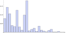
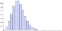
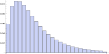
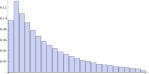
Figure 1: Initial (on the left) and long-time equilibrium (on the right) distributions for the models at issue: the first row refers to the Case FSP (fixed saving propensity), the second row to the Case TID (trading individuals dependence), the third row to the Case FAE (fixed amount exchange). Notice that the histograms are scaled differently on different pictures.

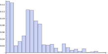
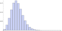
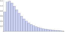
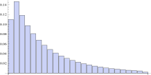
Figure 2: Initial (on the left) and long-time equilibrium (on the right) distributions for the models at issue: the first row refers to the Case FSP (fixed saving propensity), the second row to the Case TID (trading individuals dependence), the third row to the Case FAE (fixed amount exchange). Notice that the histograms are scaled differently on different pictures.

The Figures $1$ and $2$ suggest that a fat tail exists in the Cases TID and FAE, and not in the Case FSP. As a more, a log-log plot of the right section of the asymptotic stationary distributions is in agreement with a power law type decrease for the Cases TID and FAE, while this does not happen in the Case FSP.

To gain some accuracy, we tried several simulations in correspondence to a different choice of the average incomes: in particular, we took them to be nonlinear: $r_{j}=10\,(1,67)^{j}$ for $j\in\Gamma_{25}$, so as to have $r_{24}/r_{15}\sim 100$. The expectation was confirmed: no power law behavior is seen in the Case FSP, while a clear straight line appears in the log-log plots of the Cases TID and FAE. As a sample of the result of several simulations, three log-log plots relatives to the Cases FSP, TID and FAE are shown in Figure $3$.

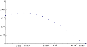
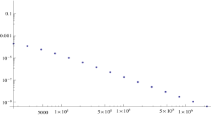
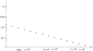
Figure 3: The (suitably rescaled) log-log plots of the right section of asymptotic stationary distributions (in a case with average incomes $r_{j}=10\,(1,67)^{j}$) in the three Cases: FSP, TID, and FAE. A clear straight line appears in the log-log plots of the Cases TID and FAE, while this does not happen in the Case FSP.

3.2 Some remarks on finding power laws

In general, simulations based on classes whose income values increase linearly do not allow a precise determination of the tail of the equilibrium distribution. It is well known (see e.g. CleGal ) that in real statistical data a fraction of less than $2$-$3$ $\%$ of the population has an income distributed according to a power law. But a power law tail can be clearly distinguished from an exponential tail only over an income range of two or three magnitude orders. This requires the introduction in our model of class incomes growing more steeply than linearly; in this way the individuals of the $25$-th class would not be, for instance, $25$ times richer than those of the first class, but at least $1000$ times richer.

In our previous work BerMod we introduced for this purpose class incomes which increase quadratically; in that case the income of the $25$-th class was $25^{2}$ times larger than the income of the first class. Notice that when the class income $r_{i}$ is not linear in the $i$-th class, a rescaling of the discrete distribution function $x_{i}$ is necessary, in order to preserve the correct relation between the distribution density and the cumulative income distribution BerMod . It is possible to check that the cumulative distribution $\sum_{i=1}^{k}x_{i}$ computed explicitly from the simulations tends to coincide for large $k$ with the integral of the rescaled density, provided one also takes into account certain slight differences in the normalization (the discrete incomes are normalized as $\sum_{i=1}^{n}x_{i}=1$, while the rescaled density $f(r)$ is normalized as $\int_{0}^{\infty}f(r)dr=1$).

In the simulations for the investigation described here we employed, besides linear class incomes, incomes which increase exponentially as $r_{i}=10\,(1,67)^{i}$. The basis 1.67 is chosen in such a way as to obtain an income increase by a factor 100 when the class index $i$ increases by 10 (the tail of the distribution is typically fitted to look for a power law in the range from $i=15$ to $i=25$). The rescaling factor to be applied to the discrete distribution function $x_{i}$ is in this case proportional to the reciprocal income $r_{i}^{-1}$; this means that a power law tail maintains, after rescaling, the same power law form, with an effective Pareto index equal to the index of the $x_{i}$ augmented by $1$.

3.3 A short survey of some wealth exchange models

To put our analysis into an historical prespective, we recall here that several mathematical models of wealth exchange processes display a Pareto tail in their equilibrium solutions. In some cases the tail has only be observed numerically, in others it is a part of an analytical solution. In some models the Pareto index is a constant, in others it depends on some parameters. Finally, some models are conservative, the conserved quantity being the total wealth; in others the total wealth increases in time.

For instance, the model by Bouchaud and Mezard BouMez , originally developed in physics for the description of polymers, admits (when the exchange rate $J$ is the same for all agents) an exact solution in the mean-field approximation. The distribution function is in that case an Amoroso curve with a Pareto index $\alpha=1+J/\sigma^{2}$ which depends on the exchange rate $J$ and on the variance $\sigma$ of a Gaussian multiplicative process appearing in the model equations. The Gaussian process simulates investment dynamics and is related to the temporal change in the value of the stocks which, on the average, increases in time.

The model by Scafetta, West and Picozzi ScaWesPic is an evolution of the model by Bouchaud and Mezard, which takes into account several realistic details of the exchange process. Its computer-generated wealth distribution functions can be fitted by rational functions of the form $f(x)=ax^{\gamma}/(1+bx)^{\gamma+\delta}$, where the Pareto index is $\alpha=\delta-1$.

In the model by Slanina Sla , growing markets are modeled by bringing in during each trading an extra amount of wealth, which is proportional to the wealth of both agents participating in the trading: this represents, realistically, the fact that the rich can invest more, and with more return. One finds in this case a power law distribution for the rich of the form $f(x)\sim x^{-1.7}$.

In the classical conservative model by Chatterjee, Chakrabarti and Manna ChattChakrManna , agents contribute only a fraction of their wealth for trading, depending on their saving propensities, which differ among agents. A Pareto tail is found, of the form $f(x)\sim x^{-2}$.

Our model family somehow resembles that one by Chatterjee, Chakrabarti and Manna ChattChakrManna . However, differently from it, it allows to recover different Pareto indices (compare e.g. results in BerMod or see the data in the caption of the Figure $4$).

The question of taxation and redistribution was first studied in DraYak , where it was modeled through a Boltzmann equation. A different approach was developed in Gua , encompassing two-step tradings, which consist of a wealth exchange analogous to an inelastic binary “collision ”and of a redistribution of the lost wealth (the taxes) among the population. The effect of the subsidies by the government on the equilibrium distribution is shown in both papers DraYak and Gua to cause a shifting of the individuals from the lower income classes toward middle income classes. Accordingly, and differently with respect to what happens e.g. to Boltzmann-Gibbs distributions, the equilibrium distribution is seen to exhibit a maximum. The Figure $5$ of DraYak and the Figure $2$ of Gua are qualitatively similar to the figures of this paper with the histograms representing the asymptotic equilibria.

4 The $\kappa$ distribution as a reasonable fit

When the equilibrium income distribution $f(x)$ of a model is found through numerical methods, it is customary to characterize this function according to its general features (e.g., monotonicity, presence of a maximum, value at zero) and to compute some global statistical indices, as the variance, the Gini index, etc.. Finally, one tries to fit $f(x)$ with some known multi-parameter distribution.

It is well known, for instance, that reversible kinetic systems evolve towards a Gibbs function, independently from the details of the transition probabilities, while non-reversible systems with fixed saving propensity evolve towards a Gamma function. For systems with a Pareto power law tail, four are, to our knowledge, the fit functions which have been proposed in the literature: the Amoroso distribution Amo , the Pareto-Gompertz distribution ChaFigMouRib , some rational functions of the form $f(x)=ax^{\gamma}/(1+bx)^{\gamma+\delta}$ScaWesPic , and the $\kappa$-generalized distribution Kan , CleGalKan , CleDiMGalKan .

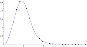
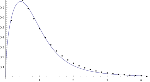
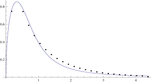
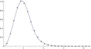
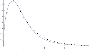
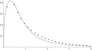
Figure 4: In each of the two panel rows three fittings are illustrated of three asymptotic stationary distributions relative to the three Cases FSP, TID, and FAE of Section 3 with the $\kappa$-generalized distribution. The taxations rates $\tau_{j}$ are different in the simulations relative to the first and to the second row. The horizontal variable is defined as $x=z/\langle z\rangle$, with $z$ the absolute personal income and $\langle z\rangle$ its mean value. The vertical variable is rescaled so as to have a normalized distribution. The parameters $\alpha,\beta$ e $\kappa$ of the $\kappa$-generalized distribution $(\ref{Kan distribution})$ are as follows. In the first row: FSP: $\alpha=2.9459$, $\beta=0.7754$, $\kappa=0.4426$; TID: $\alpha=1.5113$, $\beta=1.0574$, $\kappa=0.6156$; FAE: $\alpha=1.4601$, $\beta=1.3008$, $\kappa=0.9952$; in the second row: FSP: $\alpha=2.8868$, $\beta=0.7776$, $\kappa=0.4342$; TID: $\alpha=1.5118$, $\beta=1.0560$, $\kappa=0.6138$; FAE: $\alpha=1.3784$, $\beta=1.2171$, $\kappa=0.8664$.

The Amoroso distribution

$$f(x)=\frac{(\alpha-1)^{\alpha}}{\Gamma(\alpha)}\frac{e^{-\frac{\alpha-1}{x}}}{x^{1+\alpha}}$$

contains one parameter and is the exact limit of the model by Bouchaud and Mezard BouMez . It is characterized by the presence of a maximum, by a null value in zero (with exponential increase) and by a Pareto index $\alpha$ which is independent from the average income.

The Pareto-Gompertz distribution contains three independent parameters, is monotonically decreasing and has a Pareto index which depends on the average income. Its analytical expression is more complex: it is given by a combination of a double exponential of the form $f(x)=Be^{A-Bx}e^{e^{A-Bx}}$ followed by a power tail. It has been successfully employed e.g. in ChaFigMouRib for the description of real statistical data from Brazil.

Rational functions of the form $f(x)=ax^{\gamma}/(1+bx)^{\gamma+\delta}$ are suggested by Scafetta, West and Picozzi in ScaWesPic as apparently well fittings the computer-generated wealth distributions of their trade-investment model.

The $\kappa$-generalized distribution, given by

$$f(x)=\frac{\alpha\beta x^{\alpha-1}exp_{\kappa}(-\beta x^{\alpha})}{\sqrt{1+\beta^{2}\kappa^{2}x^{2\alpha}}}\,,$$ (8)

with the generalized exponential function

$$exp_{\kappa}(y)=(\sqrt{1+\kappa^{2}y^{2}}+\kappa y)^{1/\kappa}$$

was introduced by Kaniadakis in Kan in a general context. In CleGalKan and CleDiMGalKan it has been considered in connection with its application to the economic problem of the representation of income distribution, with the parameters $\alpha,\beta>0$ and $\kappa\in[0,1)$. In that context, the variable $x$ in $(\ref{Kan distribution})$ is defined as $x=z/\langle z\rangle$, with $z$ the absolute personal income and $\langle z\rangle$ its mean value. One of the interesting properties that this probability density function enjoys is its behavior for large values of $x$; indeed,

$$f(x)\sim{\frac{\alpha}{\kappa}\,(2\beta\,\kappa)^{-1/\kappa}}\,x^{-(\frac{\alpha}{\kappa}+1)}\qquad\hbox{for}\ x\to+\infty\,.$$

The parameters $\alpha$ and $\beta$ respectively determine the curvature (shape) and the scale of the probability distribution. The parameter $\kappa$ measures the fatness of the upper tail: the larger its magnitude is, the fatter the tail is. The strength of the $\kappa$-generalized distribution stems from its ability to reproduce in an excellent way empirical data of several countries (see CleGalKan for data concerning Germany, Italy, United Kingdom and CleDiMGalKan for Australia, United States).

Based on several attempts to fit the asymptotic stationary distributions resulting from our simulations with one or the other of the mentioned analytical expressions, we are in the position of claiming that the unique among them which seems to be suitable for the purpose is the $\kappa$-generalized distribution. In fact, it displays quite good performances.

The Figure $4$ illustrates in each of the two panel rows a sample of three fittings out of many, relative to the three Cases FSP, TID and FAE introduced in Section 3. The average incomes are $r_{j}=10j$. The taxations rates $\tau_{j}$ are taken differently in the simulations relative to the first and to the second row. Specifically, in the simulations whose asymptotic trend is shown in the first row, three taxation rates are postulated, given by:

$$\begin{array}[]{llll}\tau_{j}=5/100&\hbox{for}\ j=1,...,5\,,\\ \tau_{j}=25/100&\hbox{for}\ j=6,...,20\,,\\ \tau_{j}=45/100&\hbox{for}\ j=21,...,25\,,\end{array}$$

while in the simulations relative to the second row the taxation rates are as in $(\ref{progressivetaxrates})$. In each of the plots the horizontal variable is given by $x=z/\langle z\rangle$, with $z$ the absolute personal income and $\langle z\rangle$ its mean value and the vertical variable representing the fraction of individual with a certain income is rescaled so as to have a distribution.

5 Some remarks on reversibility

According to general results of kinetic theory Yak any system with reversible microscopic interactions approaches, at equilibrium, a Gibbs distribution function (a pure exponential). The reversibility condition is satisfied when the probability of each inverse elementary interaction process in the system is equal to the probability of the corresponding direct process.

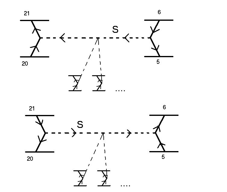
Figure 5: Example of non-reversible process with taxes. The first diagram shows an example of an interaction between a “rich”agent (belonging to the $20$-th income class) and a “poor”agent ($6$-th class). In this case the poor agent pays an amount S and acquires a definite probability to pass to the lower class. The rich agent gains an amount $S$ minus the taxes and acquires a probability to pass to the higher class. The taxes are distributed among all the other agents, giving each of them a (small) probability of transition to their upper classes. The second diagram represents the inverse process, where the rich agent pays the poor agent and thus acquires a probability to pass to the lower class. Suppose that the two alternatives “$6$ pays $20$”and “$21$ pays $5$”have the same probability. If the rich and the poor are subjected to different taxation rates, then the two diagrams have different probabilities and the whole process is clearly non-reversible. But even if the taxation rate is the same, the whole process is non-reversible, because there exists no way for all the other agents to give the tax money back. In other words, the exchange of the amount $S$ can be reversed, but not the “small re-distributions”of the tax on S.

For our model family, a typical example of elementary interaction with money exchange and taxation is shown in Fig. 5 (see detailed discussion below). This interaction is reversible in only one case among those described in this paper, and more precisely only provided the following three conditions are satisfied (see Table $1$):

1. the parameters $b^{k}_{ij}$ are as in the Case FAE of the model family, in which the exchanged amount is fixed and the saving propensity is variable;

2. the class income values $r_{j}$ are linear in the class index $j$;

3. the taxation rates are set equal to zero.

Let us analyse these three conditions in detail.

As for condition $1$, it is well known Yak and easily realised that wealth exchange processes with fixed saving propensity are non-reversible. Such processes are present in the Case FSP of our model, where $p_{hk}=(1/4)\,r_{h}/r_{n}$. In Case TID, where $p_{hk}=(1/4)\,\min\{r_{h}/r_{k}\}/r_{n}$, the interaction is also non-reversible, because the quantity $\min\{r_{h}/r_{k}\}$ is in general different in the direct process and in the inverse process.

In connection with condition $2$, we notice that the income differences $|r_{i}-r_{i-1}|$ in the denominators of the parameters $b_{hk}^{i}$ in $(\ref{bhk})$ are independent from the index $i$ only if $r_{i}$ is linear in $i$. Otherwise, the income differences depend on income, being typically larger for the rich classes. It follows that also in that case the probabilities of the direct and inverse wealth exchange processes are not the same.

Finally, about condition $3$, even assuming that the conditions conditions $1$ and $2$ hold true, we have irreversibility due to the taxation process. This can be grasped by looking at the Figure $5$, which is supposed to refer to Case FAE of our model family, with linear class incomes. The first diagram shows an example of an interaction between a “rich”agent (belonging to the $20$-th income class) and a “poor”agent ($6$-th class). In this case the poor agent pays an amount $S$ and acquires a definite probability to pass to the lower class. The rich agent gains an amount $S$ minus the taxes and acquires a probability to pass to the higher class. The taxes are distributed among all the other agents, giving each of them a (small) probability of transition to their upper classes. The second diagram represents the inverse process, where the rich agent pays the poor agent and thus acquires a probability to pass to the lower class. Plainly, if the rich and the poor are subjected to different taxation rates, then the two diagrams have different probabilities and the whole process is non-reversible. But even if the taxation rate is the same, the whole process is non-reversible, because there exists no way for all the other agents to give the tax money back. In other words, the exchange of the amount $S$ can be reversed, but not the “small redistributions” of the tax on $S$.

Hence, calculating the distribution function of our model in Case FAE, with linear income classes and no taxes, provides an important cross-check of the model and of the numerical solutions: we expect in this case to obtain the pure Gibbs distribution predicted by kinetic theory for reversible processes. And this is, actually, what is found: one obtains an exponential distribution, except for the first and last classes, whose wealth exchanges are non-reversible due to boundary effects.

In this connection we also recall that the initial conditions play in general a role in the equilibrium approach to a Gibbs distribution: such an equilibrium distribution can be reached in a conservative system only if the initial conditions do not display a population inversion corresponding to negative temperature. In our case this is guaranteed by the choice of an initial population concentrated in the classes with low income (compare Section 3).

The emergence, in the reversible case without taxes, of a purely exponential distribution is at the same time natural and puzzling. One can naturally expect, in fact, that the removal of taxes causes an increase in the population of the poorest at the detriment of the middle classes, as it happens in the exponential distribution. On the other hand, the exponential tail is thinner than the power law tail of the (non-reversible) distribution with taxes, and the reason for this is less obvious. Things go as if the complete reversibility of the wealth exchange would make it harder for the super-rich to preserve their wealth.

We close this section recalling that we pointed out in Section 3 a similarity between the Case FAE (with a fixed exchanged amount of money) of our model family and some models without taxes and with variable saving propensity (ChattChakrManna , see also PatHeinCha and MatTos ). We observed that our fixed exchanged amount of money mimics a saving propensity which varies among agents belonging to different classes and that in both cases a Pareto tail is found. Since, however, the removal of the taxes from our model causes the Pareto tail to disappear, one should conclude that the dynamical mechanism behind the formation of the tail is different in the two cases.

Table 1: Summary of results. The three basic model cases considered in this paper (first column) and their further subdivision/specialization according to taxation and linear/nonlinear class incomes. The last two columns record the appearence of reversibility and power law tails. Notice that linear class incomes in general do not allow to distinguish clearly between a power law tail and an exponential tail.

Model	Income	Reversibility	Fat tail
	linear	no	?
FSP with taxes	non-lin.	no	no
	linear	no	?
FSP, no taxes	non-lin.	no	no
	linear	no	?
TID with taxes	non-lin.	no	yes
	linear	no	?
TID, no taxes	non-lin.	no	yes
	linear	no	?
FAE with taxes	non-lin.	no	yes
	linear	yes	no
FAE, no taxes	non-lin.	no	yes

6 Concluding remarks

The aim of this paper is to provide further insight into the formation process of stationary income profiles. A family of models introduced in Ber and BerMod has been investigated. In particular, the high flexibility of these models (related to the wide range of possible parameter choices) has been exploited for the construction of various examples. A comparison between different long time behaviors exhibited by those examples contributes to further understanding of the mechanisms responsible for the emergence of one or the other output. Attention has also been given to placing our results within a frame of related results obtained through different methods.

Our approach for the description of the process of wealth exchange in the presence of taxation comprises a subdivision of the population into income classes, and a corresponding discretization of the distribution function. This approach has proven to be powerful in its application. It translates well-tested physical methods of kinetic theory into a manageable mathematical framework (a system of ordinary differential equations) which can be quickly solved numerically with standard software. The microscopic interaction parameters as well as the taxation rates have a straightforward interpretation and can be easily varied. This allows to reproduce the qualitative results of several different models.

In particular, in correspondence to some parameter choices, stationary distributions have been found, whose higher income sections exhibit a power law decreasing behavior. It could be argued in this connection that properly talking of power law tails requires treating the income or wealth variable as a continuous one taking values in $[0,+\infty)$. This is for example what is done in papers like DurMatTos and MatTos , where a rigorous analytical approach is developed, which includes the study of the evolution of the moments of the solution. Certainly, admitting a finite number of income classes entails some unnatural constraint and causes some boundary effect as well. On the other hand, we think that for the application-oriented problem at issue this is not so out of place: typically, in reports and studies concerning real world populations, income distributions are never infinitely extended, a finite number of income bins are taken into consideration, and of course, statements concerning the power law decreasing behavior are not to be intended in a strictly analytical way. We rather observe that for a more credible depiction of modern market economies, more relevant corrections should be incorporated in the model, the first one being probably the introduction of a term accounting for a possible generation of wealth due to production efficiency increase. In fact, the conservation of the total wealth is not a realistic assumption.

We are very far from thinking and claiming that the models investigated here can be employed to explain in a satisfactory way real world situations. However, they may provide a starting point for further progress in this direction. The reason for their interest, we think, is given by their flexibility and ability of reproducing the emergence of qualitative global features based only on the description of the micro-level interactions. And this is one of the main challenges in a complex systems approach.

References

- (1) A. Drăgulescu, V.M. Yakovenko, Eur. Phys. J. B, 17, (2000) 723–729.
- (2) A. Chakraborti, B.K. Chakrabarti, Eur. Phys. J. B, 17, (2000) 167–170.
- (3) F. Chami Figueira, N.J. Moura Jr., M.B. Ribeiro, Physica A 390, (2011) 689–698.
- (4) A. Chatterjee, B.K. Chakrabarti, Eur. Phys. J. B 60, (2007) 135–149.
- (5) B. Düring, D. Matthes, G. Toscani, Riv. Mat. Univ. Parma (8) 1, (2009) 199–261.
- (6) V.M. Yakovenko, in Encyclopedia of Complexity and System Science, edited by R.A. Meyer, Springer (2009), 247–272.
- (7) V.M. Yakovenko, J.B. Rosser J., Rev. Mod. Phys., 81, (2009) 1703–1725.
- (8) M.L. Bertotti, G. Modanese, Physica A, 390, (2011) 3782–3793.
- (9) M.L. Bertotti, Appl. Math. Comput., 217, (2010) 752–762.
- (10) V. Pareto, Course d’Economie Politique (Rouge, Lausanne 1896-7).
- (11) A. Chatterjee, B.K. Chakrabarti, S.S. Manna, Physica A, 335, (2004) 155–163.
- (12) M. Patriarca, E. Heinsalu, A. Chakraborti, Eur. Phys. J. B 73, (2010) 145–153.
- (13) D. Matthes, G. Toscani, J. Statist. Phys., 130, (2008) 1087–1117.
- (14) G. Kaniadakis, Physica A, 296, (2001) 405–425.
- (15) F. Clementi, M. Gallegati, G. Kaniadakis, Eur. Phys. J. B 52, (2007) 187–193.
- (16) F. Clementi, T. Di Matteo, M. Gallegati, G. Kaniadakis, Physica A, 387, (2008) 3201–3208.
- (17) F. Clementi, M. Gallegati, in Econophysics of Wealth Distributions, edited by A. Chatterjee, , S. Yarlagadda, B.K. Chakrabarti, Springer (2005), 3–14.
- (18) J.P. Bouchaud, M. Mezard, Physica A 282, (2000) 536–545.
- (19) N. Scafetta, B.J. West, S. Picozzi, Physica D 193, (2004) 338–352.
- (20) F. Slanina, Phys. Review E, 69, (2004) 046102.
- (21) S.D. Guala, Interdisciplinary Description of Complex Systems, 7, (2009) 1–7.
- (22) L. Amoroso, Ann. Mat. Pura Appl., Ser. 4 21, (1925) 123–159.