Perfect quantum transport in arbitrary spin networks

Abstract

Spin chains have been proposed as wires to transport information between distributed registers in a quantum information processor. Unfortunately, the challenges in manufacturing linear chains with engineered couplings has hindered experimental implementations. Here we present strategies to achieve perfect quantum information transport in arbitrary spin networks. Our proposal is based on the weak coupling limit for pure state transport, where information is transferred between two end-spins that are only weakly coupled to the rest of the network. This regime allows disregarding the complex, internal dynamics of the bulk network and relying on virtual transitions or on the coupling to a single bulk eigenmode. We further introduce control methods capable of tuning the transport process and achieve perfect fidelity with limited resources, involving only manipulation of the end-qubits. These strategies could be thus applied not only to engineered systems with relaxed fabrication precision, but also to naturally occurring networks; specifically, we discuss the practical implementation of quantum state transfer between two separated nitrogen vacancy (NV) centers through a network of nitrogen substitutional impurities.

Transport of quantum information between distant qubits is an essential task for quantum communication Kimble (2008) and quantum computation Cirac et al. (1997). Linear spin chains have been proposed Bose (2003) as quantum wires to connect distant computational units of a distributed quantum processor. This architecture would overcome the lack of local addressability of naturally occurring spin networks by separating in space the computational qubit registers while relying on free evolution of the spin wires to transmit information among them. Engineering the coupling between spins can improve the transport fidelity Christandl et al. (2004), even allowing for perfect quantum state transport (QST), but it is difficult to achieve in experimental systems. Remarkable work Wojcik et al. (2005); Li et al. (2005) found relaxed coupling engineering requirements – however, even these proposals still required linear chains with nearest-neighbor couplings Gualdi et al. (2008); Yao et al. (2011) or networks will all equal couplings Wójcik et al. (2007). These requirements remain too restrictive to allow an experimental implementation, since manufacturing highly regular networks is challenging with current technology Strauch and Williams (2008); Hirjibehedin et al. (2006); Spinicelli et al. (2011); Ajoy et al. (2012).

Here we describe strategies for achieving QST between separated “end”-spins in an arbitrary network topology. We employ the weak-coupling regime Wojcik et al. (2005); Li et al. (2005); Gualdi et al. (2008); Yao et al. (2011); Wójcik et al. (2007); Banchi et al. (2011), where the end-spins are engineered to be weakly coupled to the bulk of the network. We describe the transport dynamics via a perturbative approach, identifying two different regimes. Perfect transport can be achieved by setting the end-spins far off-resonance from the rest of the network – transport is then driven by a second-order process and hence is slow, but it requires no active control. Faster transport is reached by bringing the end spins in resonance with a mode of the bulk of the network, effectively creating a $\Lambda$-type network Ajoy and Cappellaro (2012a), whose dynamics we characterize completely. We further introduce a simple control sequence that ensures perfect QST by properly balancing the coupling of the end-spins to the common bulk mode, thus allowing perfect and fast state transfer. Finally, we investigate the scaling of QST in various types of networks and discuss practical implementations for QST between separated nitrogen vacancy (NV) centers in diamond Dutt et al. (2007); Jelezko and Wrachtrup (2006) via randomly positioned electronic Nitrogen impurities Barklie and Guven (1981); Hanson et al. (2008); Cappellaro et al. (2011); Yao et al. (2012).

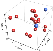
Figure 1: Example of spin network, consisting of NV centers (blue spheres) and P1 centers (red) in a diamond lattice. The network is given by randomly positioned P1 centers in the diamond lattice with a concentration of $0.2$ ppm and a $5\%$ conversion efficiency to NV. The proposed strategies enable perfect quantum state transfer between the two NV spins in this naturally occurring topology of P1 centers Cappellaro et al. (2011); Yao et al. (2012).

Spin Network –

The system (Fig. 1) is an $N$-spin network, whose nodes represent spins-$\frac{1}{2}$ and whose edges $H_{ij}$ are the Hamiltonian coupling spins $i$ and $j$. We consider the isotropic XY Hamiltonian, $H_{ij}=(S_{i}^{+}S_{j}^{-}+S_{i}^{-}S_{j}^{+})$, with $S_{j}^{\pm}=\frac{1}{2}(S^{x}_{j}\pm iS^{y}_{j})$, which has been widely studied for quantum transport Ajoy and Cappellaro (2012a); Cappellaro et al. (2007); Bose (2003); Benjamin and Bose (2003). We further assume that two nodes, labeled 1 and $N$, can be partially controlled and read out, independently from the bulk of the network: we will consider QST between these end spins. For perfect transport, an excitation created at the location of spin $1$ should be transmitted without distortion to the position of spin $N$ upon evolution under $H$. We characterize the efficiency of transport by the fidelity, $F(t)=|\left\langle{N}\right|e^{-iHt}\left|{1}\right\rangle|^{2}$, where $\left|{j}\right\rangle$ represents a single excitation $\left|{1}\right\rangle$ at spin $j$, while all other spins are in the ground state $\left|{0}\right\rangle$.

Weak-coupling regime –

While optimal fidelity has been obtained for particular, engineered networks (mainly 1D, nearest-neighbor chains), here we consider a completely arbitrary bulk network, $H_{B}$. To ensure perfect transport, we work in the weak-coupling regime for the end-spin coupling $H_{e}$. By engineering appropriate weights $\epsilon,\bm{\beta}$, we thus impose $\epsilon\|H_{e}\|\ll\bm{\beta}\|H_{B}\|$, where $\|\cdot\|$ is a suitable matrix norm Bhatia (1996).

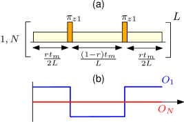
Figure 2: (a) On-resonance balancing sequence applied to the end spins for perfect quantum transport. Yellow blocks indicate microwave irradiation that brings the end spins on resonance with the bulk network. The resulting $\Lambda$-network is in general unbalanced, but appropriately placed $\pi$-pulses (orange) on the end-spin with higher mode overlap (here spin 1) can balance the overlaps $O_{(1,N)}$ Ajoy et al. (2011). (b) The $\pi$-pulses invert the sign of spin-1 coupling to the bulk mode in the toggling frame such that $O_{1,N}$ become equal on average. For the network of Fig. 1, $|O_{1}|\!>\!|O_{N}|$ and $r\!=\!1/2(1+|O_{N}/O_{1}|)=0.5501$. The sequence is symmetrized Levitt (2008); Suzuki (1990) and repeated for $L$ cycles.

Intuitively, we expect the weak coupling regime to achieve perfect transfer since it imposes two rates to the spin dynamics: the bulk spins evolve on a “fast” time scale while the end-spin dynamics is “slow”. The end spins inject information into the bulk, which evolves so quickly that information spreads everywhere at a rate much faster than new information is fed in, allowing an adiabatic elimination of the information quantum walk in the bulk network Ajoy and Cappellaro (2012a); Cohen-Tannoudji et al. (1992). Although high fidelity can be reached, this off-resonance transport is very slow.

A different strategy, and a faster rate, for information transport is achieved by bringing the end-spins on resonance with an eigenmode of the bulk – the weak coupling ensuring greater overlap with a single (possibly degenerate) mode. The system reduces to a $\Lambda$-network Ajoy and Cappellaro (2012a), where coupled-mode theory ensures perfect transport if both ends have equal overlaps with the bulk mode Haus and Huang (1991); Synder and Love (1983), a condition that we will show can be engineered by the control sequence in Fig. 2.

To make more rigorous our intuition of the weak regime, we describe transport via a perturbative treatment. For convenience we consider normalized matrices, $\|H_{B}\|\!=\!\|H_{e}\|\!=\!1$, and introduce the network adjacency matrix, $A\!=\!\bm{\beta}A^{B}\!+\!\epsilon A^{e}$, which describes the coupling networks of the system Hamiltonian $H\!=\!\bm{\beta}H_{B}+\epsilon H_{e}$. Transport in the single excitation subspace is fully described by $A$ Christandl et al. (2004), thus the fidelity can be written as $F(t)=|\left\langle{N}\right|e^{-iAt}\left|{1}\right\rangle|^{2}$, where the vectors $\left|{j}\right\rangle$ now represent the node basis in the $N\times N$ network space. We use a Schrieffer-Wolff transformation Schrieffer and Wolff (1966); Bravyi et al. (2011) and its truncation to first order in $\epsilon/\bm{\beta}$ to define an effective adjacency matrix, $A^{\prime}=e^{S}Ae^{-S}\approx A+\frac{1}{2}[S,A]$, which drives the evolution. Setting $S$ so that $[A^{B},S]=\frac{\epsilon}{\bm{\beta}}A^{e}$, we have $A^{\prime}\approx\bm{\beta}A^{B}+\frac{\epsilon}{2}A^{S}$, where $A^{S}\!=\![S,A^{e}]$ can be evaluated explicitly.

Off-resonance QST –

Consider first the case where the eigenvalues $\{E_{j}^{B}\}$ of $A^{B}$ are non-degenerate, except for $E_{1}^{B}\!=\!E_{N}^{B}\!=\!0$ (associated with the end-spin subspace). We can fix the energy eigenbasis $\{\left|{v_{k}}\right\rangle\}$ of $A^{B}$ by setting $\left|{v_{1}}\right\rangle=\left|{1}\right\rangle$ and $\left|{v_{N}}\right\rangle=\left|{N}\right\rangle$. In this basis the structure of the matrix $A^{e}$ is preserved, non-zero terms connecting only the ends to the bulk, $A^{e}_{\ell,j}=0$ for $\ell\neq 1,N$. A general element of $A^{S}$ can be written as,

$$A^{S}_{ij}=\frac{\epsilon^{2}}{\bm{\beta}}\sum_{k}A^{e}_{ik}A^{e}_{kj}\left(\frac{1}{E_{i}^{B}-E_{k}^{B}}+\frac{1}{E_{j}^{B}-E_{k}^{B}}\right)$$

Given the form of $A^{e}$, we have, for $\{i,j\}\neq 1,N$,

$$A^{S}_{ij}=\frac{\epsilon^{2}}{\bm{\beta}}(A_{i1}A_{1j}+A_{iN}A_{Nj})\left(\frac{1}{E_{i}^{B}}+\frac{1}{E_{j}^{B}}\right).$$ (1)

Also, setting $k\neq 1,N$ and $\{\zeta,\xi\}\in\{1,N\}$ we have

$$A^{S}_{\zeta\xi}=-\textstyle\frac{2\epsilon^{2}}{\bm{\beta}}\sum_{k}A^{e}_{\zeta k}A^{e}_{k\xi}/{E^{B}_{k}},$$ (2)

while if $A^{e}_{\xi,\zeta}=0$ elements between the end and bulk are zero, $A^{S}_{\zeta k}=0$.

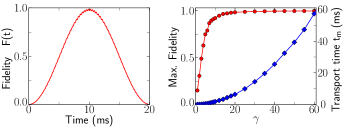
Figure 3: (a) Off-resonance transport fidelity for the network in Fig. 1 for $\gamma=25$. Perfect transport occurs, but on a slow time scale, an order of magnitude longer than the on-resonance balanced case (Fig. 4). (b) Increasing $\gamma$ improves transport fidelity (red circles) but also increases the time required for perfect transport (blue diamonds).

Hence $A^{S}$ can be partitioned into a term with support only in the bulk subspace (Eq. 1) and a second term with support only in the end-spin subspace (Eq. 2), while there is no end-bulk coupling. To first order approximation, it is only the latter term that drives QST – the transport happens via a direct coupling between the end-nodes. Since this effective coupling is mediated by the bulk via virtual transitions, its rate is proportional to $\epsilon^{2}/\bm{\beta}$. The fidelity of transport is determined entirely by the effective detuning of the two end-spins, $\alpha=(A^{S}_{11}-A^{S}_{NN})/2$:

$$F(t)=\frac{(A^{S}_{1N})^{2}}{(A^{S}_{1N})^{2}+\alpha^{2}}\sin^{2}\left(t\sqrt{(A^{S}_{1N})^{2}+\alpha^{2}}\right)$$ (3)

If we can modify the end-spin Hamiltonian by adding a term $H_{\text{off}}=-2(\omega_{1}S^{z}_{1}+\omega_{N}S^{z}_{N})$, such that $A^{S}_{11}+\omega_{1}=A^{S}_{NN}+\omega_{N}$, perfect quantum transport is ensured at $t_{m}=\pi/(2A^{S}_{1N})$. This energy shift could be obtained by locally tuning the magnetic field or by applying local AC driving, ensuring the desired energy in the rotating frame (similar to the Hartman-Hahn scheme Hartman and Hahn (1962)). Transport fidelity also depends on the goodness of the first order approximation, increasing with $\bm{\beta}/\epsilon$ as shown in Fig. 3(b) at the cost of longer transport times.

On-resonance QST

– Transport can be made faster if the end spins are on resonance with one non-degenerate mode of the bulk $\left|{v_{d}}\right\rangle$ (we will consider the degenerate case in SOM ). Resonance happens if the corresponding eigenvalue $E_{d}^{B}=0$ or it can be enforced by adding an energy shift to the end spins to set $A^{e}_{11}=A^{e}_{NN}=\bm{\beta}/\epsilon E^{B}_{d}$. Transport then occurs at a rate proportional to $\epsilon$, as driven by the adjacency matrix $A^{d}$, the projection of $A^{e}$ in the degenerate subspace:

$$A^{d}=\left\langle{1}\right|A^{e}\left|{v_{j}}\right\rangle\left|{1}\right\rangle\!\!\left\langle{v_{d}}\right|+\left\langle{N}\right|A^{e}\left|{v_{d}}\right\rangle\left|{N}\right\rangle\!\!\left\langle{v_{d}}\right|+h.c.$$

We note that the goodness of this approximation depends on the gap between the selected resonance mode and the other bulk modes. In the node basis, $A^{d}$ forms an effective $\Lambda$-network Ajoy and Cappellaro (2012a), coupling the end-spins with each spin of the bulk:

$$A^{d}=\sum_{j}(\delta_{1j}\left|{1}\right\rangle\!\!\left\langle{j}\right|+\delta_{Nj}\left|{N}\right\rangle\!\!\left\langle{j}\right|+h.c.),$$ (4)

where $\delta_{(1,N)j}=\langle{v_{d}}|{j}\rangle\left\langle{(1,N)}\right|A^{e}\left|{v_{d}}\right\rangle$. Note that importantly we have $\delta_{1j}/\delta_{Nj}=\text{cst.}$, $\forall j$. Transport in such $\Lambda$-networks occurs at only four frequencies SOM , $F(t)=w_{0}+\sum_{m=1}^{4}w_{m}\cos(f_{m}t)$ with,

$$f_{1,2}=2\sqrt{S^{2}\mp\sqrt{S^{4}-\Delta^{4}}}\>;\>f_{3,4}=\sqrt{2(S^{2}\mp\Delta^{2})},$$ (5)

where,

$$S^{2} = \sum_{j}\frac{1}{2}(\delta_{1j}^{2}+\delta_{jN}^{2})$$

$$\Delta^{4} = \sum_{j<k}(\delta_{1j}\delta_{kN}-\delta_{jN}\delta_{1k})^{2}$$ (6)

$$\delta^{2} = \sum_{j}\delta_{1j}\delta_{jN}$$

Physically, $S\sim\|A^{d}\|$ sets the energy scale of the resonant mode, while $\Delta$ quantifies the relative detuning between different $\Lambda$-paths Ajoy and Cappellaro (2012a); SOM . The coefficients $w_{i}$ are found to be $w_{0}=-w_{3}=-w_{4}=\frac{\delta^{4}}{4(S^{4}-\Delta^{4})}$, $w_{1}=w_{2}={w_{0}}/2$, giving the analytical expression for QST in a $\Lambda$-network,

$$F(t)\!=\!\frac{\delta^{4}}{S^{4}-\Delta^{4}}\sin^{2}\!\left(\!\!\sqrt{\frac{S^{2}+\Delta^{2}}{2}}t\!\right)\!\sin^{2}\!\left(\!\!\sqrt{\frac{S^{2}-\Delta^{2}}{2}}t\!\right)$$ (7)

Perfect QST requires $\Delta=0$ and $\delta=S$. The first condition entails $\delta_{1j}/\delta_{jN}=\textrm{cst.}$ $\forall j$, which is always satisfied by $A^{d}$ if the resonant bulk mode is non-degenerate. On the other hand, $\delta=S$ requires a balanced network, $\delta_{1j}=\delta_{jN}$ $\forall j$. For the reduced adjacency matrix $A^{d}$ this condition is satisfied when both end-spins have equal overlap with the resonant eigenmode, $\left\langle{1}\right|A^{e}\left|{v_{d}}\right\rangle=\left\langle{N}\right|A^{e}\left|{v_{d}}\right\rangle$, and we show below that this can be always arranged for a non-degenerate mode by a simple control sequence (see Fig. 2). In the balanced case the fidelity simplifies to $F(t)=\sin(St/\sqrt{2})^{4}$, which leads to perfect QST at $t_{m}=\pi/(\sqrt{2}S)$, as if it were a 3-spin chain Christandl et al. (2004).

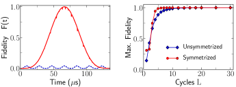
Figure 4: (a) On-resonance transport fidelity for the network of Fig. 1, with (red) and without (blue, dotted) balancing, with $\gamma=1$ and $L=20$. Almost perfect transport occurs in the balanced case, obtained by the control sequence in Fig. 2. (b) Increasing the number of cycles $L$ improves the Trotter approximation yielding enhanced fidelity. The symmetrized sequence performs better than the sequence without symmetrization.

Perfect QST by on-resonance balancing

– Unfortunately the overlaps of the two end spins with the on-resonance mode, $O_{(1,N)}=\langle{(1,N)}|A^{e}|{v_{d}}\rangle$, are in general unequal, and the $\Lambda$-network unbalanced. Still, it is possible to balance the network by a simple control sequence (Fig. 2). Assume for example $O_{1}>O_{N}$; we partition $A^{d}$ into effective adjacency matrices with couplings only to spins 1 and $N$, $A^{d}=A^{d}_{1}+A^{d}_{N}$. A rotation $e^{-iS^{z}_{1}\pi}$ on spin 1 produces $\tilde{A}^{d}=-A^{d}_{1}+A^{d}_{N}$. Then the evolution, $e^{-iA^{d}rt}e^{-i\tilde{A}^{d}(1-r)t}\!\approx\!e^{-iA^{d}_{b}t}$, with $A^{d}_{b}=A^{d}r+\tilde{A}^{d}(1\!-\!r)$, is balanced on average during the period $t$ if $r=\frac{1}{2}(1+\left|O_{N}/O_{1}\right|)$. The approximation improves if one uses $L$ cycles of the control sequence with shorter time intervals (as in a Trotter expansion Trotter (1959); Suzuki (1990)) and appropriately symmetrizes it (see Fig. 2) to achieve an error ${\cal O}({r^{2}(1-r)t_{m}^{3}}/{L^{3}})$. Fig. 4(a) shows the effect of enhanced, almost perfect, fidelity upon balancing the network of Fig. 1.

Transport time and control requirements

– We now consider the scaling of the weak coupling parameter $\gamma=\frac{\bm{\beta}}{\epsilon}$ required for the validity of the perturbative approximation. We can fix $\bm{\beta}=\|H_{B}\|$ and consider normalized matrices. Then $\bm{\beta}$ scales as $\sqrt{(N-2)(N-3)/3}$ for a random network where all the couplings are uniformly distributed. For the more realistic case where the coupling strength decreases with distance, the scaling is less favorable, e.g. for a random dipolar coupled network $\bm{\beta}$ scales as $\sqrt{2/3(N-3)}/d^{3}$, where $d$ is the average lattice constant SOM . Similar scaling occurs for regular spin networks, for example those corresponding to crystal lattices SOM . In general the ratio $\epsilon/\bm{\beta}$ decreases with the size of the network (usually as ${\cal O}(\sqrt{N})$), averting the need to reduce the end-couplings by engineering $\epsilon$. This is evident in Fig. 4, where $\epsilon=1$ is sufficient to drive perfect quantum transfer.

In the case of on-resonance balancing the time at which perfect QST is achieved is $t_{m}=\gamma\pi/(\sqrt{2}S)$, where $S=\textrm{min}\{O_{1},O_{N}\}$, scales linearly with $\gamma$. The time is shorter the more symmetrical the end-spins are with respect to the resonant mode SOM , since then $|O_{1}|\approx|O_{N}|$. For the off-resonance case the time is $t_{m}=(\pi\bm{\beta}/2\epsilon^{2})[E_{\ell}^{B}/(A^{e}_{1\ell}A^{e}_{k\ell})]$, where $E^{B}_{\ell}=\textrm{min}\{\left|E^{B}_{k}\right|\}$ is the minimum eigenvalue of the bulk. In general this second order transport process takes an order of magnitude longer time than the on-resonance case (Fig. 3).

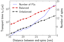
Figure 5: Time for optimal transport in dipolar coupled spin networks of P1 centers in diamond. The optimal time was calculated from the average over 5000 random lattice realizations of P1 centers of density 10ppm; we considered transport between two NV centers located at increasing distance. The red line (circles) is the time required to achieve a transport fidelity of at least 99% via resonant balancing. The black line (diamonds) is the time at which optimal fidelity is achieved for on-resonant transport without balancing. The fidelity is however quite low ($\sim\!15\%$) in this case. The blue dashed line shows the number of P1 centers in the network, $N\!-\!2$.

Finally, let us estimate the resources needed to impose the end-spin energy shifts as required for perfect QST, for example by a continuous irradiation during $t_{m}$ (Fig. 2). In the on-resonance case, the end-spin energy should be set equal to a bulk mode, $E^{B}_{d}$. Selecting the highest bulk eigenmode, which has usually the largest gap to the other modes, $E^{B}_{d}$ scales as ${\cal O}(N)$ for random networks, but it is constant, $\sim 1.6/d^{3}$, for dipolar coupled networks SOM . Off-resonance transport requires instead a shift of $A^{S}_{11}-A^{S}_{NN}$, where $A^{S}_{11,NN}=\langle{A^{e}_{1,N}}|{\ell}\rangle^{2}/\gamma^{2}E^{B}_{\ell}$, where $E^{B}_{\ell}$ is the minimum bulk eigenmode. Hence the control required in this case is about an order of magnitude lower than in the resonant case.

An experimentally important quantum computing architecture is that of nitrogen vacancy (NV) centers in diamond. Fig. 5 shows the scaling of the transport time between two separated NV centers via a bulk network consisting of randomly positioned nitrogen impurities (P1 centers). Some experimental challenges remain: the limitation of pure state transfer requires that the system is at low temperature or that P1 centers are indirectly polarized by the NV centers; the requirement of using the isotropic XY Hamiltonian requires additional control for it to be generated from the natural dipolar Hamiltonian (for example via a combination of gradient and TOCSY mixing Braunschweiler and Ernst (1983); Yao et al. (2012); Ajoy and Cappellaro (2012b)). Still, considering that dephasing times in excess of 100$\mu$s are routinely achievable Stanwix et al. (2010); Balasubramanian et al. (2009), the balanced transport scheme may be experimentally viable for quantum communication in these architectures.

Conclusion –

In this paper, we showed that perfect quantum state transfer can be engineered even in the case of arbitrarily complicated network topologies, if the ends of the network are weakly coupled to the bulk. Transport speed can be improved by bringing the end spins on resonance with a common mode of the bulk network. Alternatively, it is possible to achieve unit transport fidelity, with lower control requirements, but on a longer time scale, by detuning the end-spins off-resonance. These transport strategies may allow the interlinking of quantum registers in a quantum information processor with very relaxed fabrication requirements.

Acknowledgments –

This work was partially funded by NSF under grant DMG-1005926 and by AFOSR YIP.

Appendix A Transport for end-spins on-resonance with a degenerate mode

In the main text we described transport when the end spins are on resonance with an eigenmode of the bulk with eigenvalue $E^{B}_{d}$. Here we generalize to the situation where the eigenvalue is degenerate, with eigenvectors $\left|{\alpha_{m}}\right\rangle$. The projector onto the degenerate eigenspace is then,

$$P=(\left|{1}\right\rangle\left\langle{1}\right|+\left|{N}\right\rangle\left\langle{N}\right|)+\sum_{m\in M}\left|{\alpha_{m}}\right\rangle\left\langle{\alpha_{m}}\right|\equiv(\left|{1}\right\rangle\left\langle{1}\right|+\left|{N}\right\rangle\left\langle{N}\right|)+P_{M},$$ (8)

and, to first order, transport is driven by the projection of the adjacency matrix $A^{e}$ into the this subspace, i.e., $A^{d}=P^{{\dagger}}A^{e}P$. Now we consider that $A^{e}$ and $A^{B}$ have the following forms, where “$\times$” denotes a non-zero element:

$$A^{e}=\left[\begin{array}[]{cccccc}{}\hfil&{\times}&{\times}&{\times}&{\times}&{}\hfil\\ {\times}&{}\hfil&{}\hfil&{}\hfil&{}\hfil&{\times}\\ {\times}&{}\hfil&{}\hfil&{}\hfil&{}\hfil&{\times}\\ {\times}&{}\hfil&{}\hfil&{}\hfil&{}\hfil&{\times}\\ {\times}&{}\hfil&{}\hfil&{}\hfil&{}\hfil&{\times}\\ {}\hfil&{\times}&{\times}&{\times}&{\times}&{}\hfil\end{array}\right]\>;\>\qquad A^{B}=\left[\begin{array}[]{cccccc}}{\hfil&{}\hfil&{}\hfil&{}\hfil&{}\hfil&{}\hfil\\ {}\hfil&{}\hfil&{\times}&{\times}&{\times}&}{\hfil\\ {}\hfil&{\times}&{}\hfil&{\times}&{\times}&{}\hfil\\ {}\hfil&{\times}&{\times}&{}\hfil&{\times}&{}\hfil\\ {}\hfil&{\times}&{\times}&{\times}&{}\hfil&{}\hfil\\ {}\hfil&{}\hfil&{}\hfil&{}\hfil&{}\hfil&{}\hfil\end{array}\right].$$ (9)

It follows that

$$\langle{1}|A^{e}|{1}\rangle=0\>;\>\langle{N}|A^{e}|{N}\rangle=0\>;\>\langle{\alpha_{m^{\prime}}}|A^{e}|{\alpha_{m}}\rangle=0,$$ (10)

yielding

$$A^{d}=\sum_{m}\langle{1}|A^{e}|{\alpha_{m}}\rangle(\left|{1}\right\rangle\left\langle{\alpha_{m}}\right|+\left|{\alpha_{m}}\right\rangle\left\langle{1}\right|)+\sum_{m}\langle{N}|A^{e}|{\alpha_{m}}\rangle(\left|{N}\right\rangle\left\langle{\alpha_{m}}\right|+\left|{\alpha_{m}}\right\rangle\left\langle{N}\right|),$$ (11)

where we have used the fact that $A^{e}$ is real, and hence $\langle{1}|A^{e}|{\alpha_{m}}\rangle=\langle{\alpha_{m}}|A^{e}|{1}\rangle$. Let us define the end connection vectors,

$$A^{e}\left|{1}\right\rangle=\left|{n_{1}}\right\rangle\>;\>A^{e}\left|{N}\right\rangle=\left|{n_{N}}\right\rangle.$$ (12)

Then,

$$A^{d} = \sum_{m}\langle{n_{1}}|{\alpha_{m}}\rangle(\left|{1}\right\rangle\left\langle{\alpha_{m}}\right|+\left|{\alpha_{m}}\right\rangle\left\langle{1}\right|)+\sum_{m}\langle{n_{N}}|{\alpha_{m}}\rangle(\left|{N}\right\rangle\left\langle{\alpha_{m}}\right|+\left|{\alpha_{m}}\right\rangle\left\langle{N}\right|)$$

$$= \sum_{j}\sum_{m}\langle{n_{1}}|{\alpha_{m}}\rangle\left(\langle{\alpha_{m}}|{j}\rangle\left|{1}\right\rangle\left\langle{j}\right|+\langle{j}|{\alpha_{m}}\rangle\left|{j}\right\rangle\left\langle{1}\right|\right)+\sum_{j}\sum_{m}\langle{n_{N}}|{\alpha_{m}}\rangle\left(\langle{\alpha_{m}}|{j}\rangle\left|{N}\right\rangle\left\langle{j}\right|+\langle{j}|{\alpha_{m}}\rangle\left|{j}\right\rangle\left\langle{N}\right|\right)$$

or simplifying,

$$A^{d}=\sum_{j}(\delta_{1j}\left|{1}\right\rangle\left\langle{j}\right|+\delta_{jN}\left|{N}\right\rangle\left\langle{j}\right|+h.c.),$$ (13)

where $\delta_{(1,N)j}=\langle{n_{(1,N)}}|P_{M}|{j}\rangle$ is the overlap of the end vector $n_{1}$ and the node $j$ in the resonant subspace.

To achieve balanced on-resonance transport we require that $\delta_{1j}=\delta_{jN}$ for all $j$, which implies that both the end-vectors have equal projections in the resonant subspace,

$$P_{M}\left|{n_{1}}\right\rangle=P_{M}\left|{n_{N}}\right\rangle.$$ (14)

Appendix B Transport Fidelity for $\Lambda$-networks

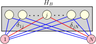
Figure 6: (Color online) A general detuned $\Lambda$-network with multiple $\Lambda$-paths between the end spins. Each leg of any of these $\Lambda$-paths may have an arbitrary detuning. For the representative case of the $\Lambda$-path going through node $j$ (red), these detunings are $\delta_{1j}$ and $\delta_{jN}$.

Here we derive the maximum transport fidelity for a $\Lambda$-type network. $\Lambda$-type networks are interesting because the effective Hamiltonian of more complex networks reduces to $\Lambda$-network Hamiltonian in the weak-coupling regime (as shown in the previous section), but we will consider here the general case.

For any network of adjacency matrix $A$, the fidelity function $F(t)\!=\!|\!\left\langle{N}\right|e^{-iAt}\left|{1}\right\rangle\!|^{2}$ has a simple expression in the eigenbasis of $A$,

$$F(t)\!=\sum_{k,\ell}\langle{\ell}|{N}\rangle\langle{N}|{k}\rangle\langle{k}|{1}\rangle\langle{1}|{\ell}\rangle\cos\left(E_{k}-E_{\ell}\right)t.$$ (15)

This shows that the fidelity can be written as the sum

$$F(t)=\sum_{n}w_{n}\cos(f_{n}t),\qquad\textrm{with}\quad f_{n}=E_{k}-E_{\ell},$$ (16)

that is, the frequencies are differences between eigenvalues of $A$, for which the corresponding eigenvectors $\left|{\ell}\right\rangle$ and $\left|{k}\right\rangle$ have non-zero overlap with $\left|{1}\right\rangle,\left|{N}\right\rangle$.

We now consider a general $\Lambda$-network with multiple $\Lambda$-paths that connect the end-spins (see Fig. 6) and we will restrict the analysis to the adjacency matrix obtained in the on-resonance case only later. We write the adjacency matrix in terms of the coupling strength $\delta_{1j}$ and $\delta_{jN}$ between the end spin and each $j^{th}$ spin in the bulk, which form the $\Lambda$ path:

$$A^{d}=\sum_{j}\Lambda_{j}\>,\qquad\Lambda_{j}=\delta_{1j}\left(\left|{j}\right\rangle\!\!\left\langle{1}\right|+\left|{1}\right\rangle\!\!\left\langle{j}\right|\right)+\delta_{jN}(\left|{j}\right\rangle\!\!\left\langle{N}\right|+\left|{N}\right\rangle\!\!\left\langle{j}\right|).$$ (17)

Our strategy for finding the transport fidelity in $\Lambda$-networks is to first determine the eigenvalues of the adjacency matrix in Eq. (17) and hence the possible frequencies at which information transport can occur. Then, we will use a series expansion to find an explicit expression for the fidelity.

B.1 Frequency of Transport

The eigenvalues of the adjacency matrix in Eq. (17) are

$$\lambda_{0} = 0,\qquad(N-4)\text{ degenerate}$$

$$\lambda_{1,2} = \pm\sqrt{S^{2}-\sqrt{S^{4}-\Delta^{4}}},$$ (18)

$$\lambda_{3,4} = \pm\sqrt{S^{2}+\sqrt{S^{4}-\Delta^{4}}},$$

where we defined,

$$S^{2} = \sum_{j}S^{2}_{j}=\sum_{j}\frac{1}{2}(\delta_{1j}^{2}+\delta_{jN}^{2})$$

$$\Delta^{4} = \sum_{j<k}\Delta_{jk}^{4}=\sum_{j<k}(\delta_{1j}\delta_{kN}-\delta_{jN}\delta_{1k})^{2}$$ (19)

$$\delta^{2} = \sum_{j}\delta_{1j}\delta_{jN}$$

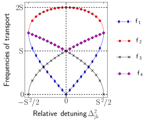
Figure 7: (Color online) Positive frequencies of transport fidelity for a $\Lambda$-network (Fig. 6) consisting of two $\Lambda$-paths, $1\to j\to N$ and $1\to k\to N$. The frequencies are plotted as a function of the relative detuning between the paths, $\Delta_{jk}^{2}=(\delta_{1j}\delta_{kN}-\delta_{jN}\delta_{1k})$. The actual transport also contains symmetric negative frequencies and a DC (zero frequency) component. In general there are four frequencies of transport, derived in Eq. (20). Note that when $\delta_{jN}/\delta_{1j}$ is a constant for both paths, there are only two frequencies, $S$ and $2S$, that carry the transport.

While for a general network the frequencies of transport are differences between the eigenvalues of $A^{d}$, here there are only four distinct frequencies because of the symmetries in the eigenvalues:

$$\begin{array}[]{l}f_{0}=0,\qquad\qquad f_{1}=2\lambda_{1},\qquad\qquad f_{2}=2\lambda_{3},\\ f_{3}=\lambda_{1}-\lambda_{3}=\sqrt{2(S^{2}-\Delta^{2})},\quad f_{4}=\lambda_{1}+\lambda_{3}=\sqrt{2(S^{2}+\Delta^{2})}.\end{array}$$ (20)

B.2 Series expansion

With the frequencies found above, equation Eq. (16) reduces to $F(t)=\sum_{i=0}^{4}w_{i}\cos{(f_{i}t)}$. To find the parameters $w_{i}$, we equate the Taylor expansion of Eq. (16) and of the fidelity $F(t)\!=\!|\!\left\langle{N}\right|e^{-iAt}\left|{1}\right\rangle\!|^{2}$. We only need the first five even power coefficients to fully determine $\{w_{i}\}$, giving the series of equations,

$$\sum_{i=0}^{4}w_{i}\!=\!|\langle{N}|{1}\rangle|^{2}=0$$

$$\sum_{i=1}^{4}w_{i}f_{i}^{2}\!=\!-|\langle{N}|A^{d}|{1}\rangle|^{2}=0$$

$$\frac{1}{4!}\sum_{i=0}^{4}w_{i}f_{i}^{4}\!=\!\frac{1}{4}|\langle{N}|\left(A^{d}\right)^{2}|{1}\rangle|^{2}=\mathcal{C}_{4}$$ (21)

$$\frac{1}{6!}\sum_{i=0}^{4}w_{i}f_{i}^{6}\!=-\!\frac{1}{24}\text{Re}[\langle{N}|\left(A^{d}\right)^{2}|{1}\rangle\langle{N}|\left(A^{d}\right)^{4}|{1}\rangle]=\mathcal{C}_{6}$$

$$\frac{1}{8!}\sum_{i=0}^{4}w_{i}f_{i}^{8}\!=\!\frac{1}{4!}|\langle{N}|\left(A^{d}\right)^{4}|{1}\rangle|^{2}+\frac{1}{2\cdot 6!}\text{Re}[\langle{N}|\left(A^{d}\right)^{2}|{1}\rangle\langle{N}|\left(A^{d}\right)^{6}|{1}\rangle]=\mathcal{C}_{8}$$

The expectation values can be evaluated exactly, yielding

$${\cal C}_{4} = \frac{1}{4}\delta^{4}$$

$${\cal C}_{6} = -\frac{1}{12}S^{2}\delta^{4}$$ (22)

$${\cal C}_{8} = \frac{1}{720}\delta^{2}\left[9S^{4}-\Delta^{2}\right]$$

For general frequencies $f_{i}$, the coefficients $w_{i}$ are

$$w_{0}=-\sum_{j=1}^{4}w_{j}; \qquad w_{j}=\frac{\mathcal{C}_{8}-\sum_{k\neq j}f_{k}^{2}\mathcal{C}_{6}+\sum_{\ell<m;\ell,m\neq j}f_{\ell}^{2}f_{m}^{2}\mathcal{C}_{4}}{f_{j}^{2}\prod_{k\neq j}(f_{k}^{2}-f_{j}^{2})}, j>0$$ (23)

Using the expressions for the frequencies in Eq. (20), we find their explicit expressions in terms of $S,\Delta$ and $\delta$:

$$w_{0}=\frac{\delta^{4}}{4(S^{4}-\Delta^{4})},\qquad w_{1}=w_{2}=\frac{w_{0}}{2},\qquad w_{3}=w_{4}=-w_{0}$$ (24)

The fidelity is thus further simplified to

$$F(t)=\frac{\delta^{4}}{S^{4}-\Delta^{4}}\left[\sin\left(t\sqrt{(S^{2}+\Delta^{2})/2}\right)\sin\left(t\sqrt{(S^{2}-\Delta^{2})/2}\right)\right]^{2}$$ (25)

B.3 Fidelity for random and degenerate networks

Consider the case when the number of nodes is large, and the detunings $\delta_{1j}$ and $\delta_{jN}$ are sampled from the same distribution, as it would be in a random network. Then,

$$\sum_{j}\delta_{1j}^{2}\approx\sum_{j}\delta_{jN}^{2}$$ (26)

since the second moments of the random distribution should be equal. In this situation we have

$$S^{4}-(\Delta^{4}+\delta^{4})=\frac{1}{4}\left[\sum_{j}(\delta_{1j}^{2}-\delta_{jN}^{2})\right]^{2}=0$$ (27)

Then the condition

$$\delta^{4}=S^{4}-\Delta^{4}$$ (28)

is satisfied and the fidelity becomes

$$F(t)=\left[\sin\left(t\sqrt{(S^{2}+\Delta^{2})/2}\right)\sin\left(t\sqrt{(S^{2}-\Delta^{2})/2}\right)\right]^{2}$$ (29)

In the case of resonance to a non-degenerate mode, we have $\Delta=0$ and the fidelity can reach its maximum $F(t)=\sin({St}/{\sqrt{2}})^{4}=1$, for $t=\pi/\sqrt{2}S$.

For the case of interest in this work, a network where the end-spins are on resonance with a non-degenerate mode, the adjacency matrix of relevance in the weak regime is the reduced adjacency matrix, $A^{d}$. As shown above, in this case we have $\Delta=0$ and the fidelity reduces to

$$F(t)=\left[\frac{\delta}{S}\sin\left(\frac{St}{\sqrt{2}}\right)\right]^{4},$$ (30)

thus maximum fidelity can be reached only if the condition Eq. (28) is satisfied. For example, the mirror-symmetric case $\delta_{1j}=\delta_{jN},\ \forall j$ yields the optimal fidelity $F=1$ since then $\delta=S$.

Appendix C Estimating matrix norms for different network topologies

C.1 Different kinds of networks

In this section, we consider different classes of networks, and estimate the norms of the corresponding adjacency matrices $A$. As described in the main text, the matrix norm of the bulk adjacency matrix is important in predicting the transport time. For example, the scaling of transport time is linear with $\gamma$ in the on-resonance case; and the value of $\gamma$ implicitly depends on the norm of the bulk matrix. Hence a large bulk matrix causes an intrinsically high $\gamma$, and reduces the control requirements on the end-spins. All the networks considered are of $N$ spins, and hence the adjacency matrices are $N\times N$ matrices.

1. Random network: The matrix $A$ has random entries in the range $[0,1]$ (with appropriate symmetrization). The random entries follow a uniform distribution, with no site-to-site correlation. Overall, this case represents a rather unphysical scenario, but will be useful in the computations that follow.

2. Random network with $1/d^{3}$ scaling: $A$ contains random entries from a uniform distribution scaled by $1/(hd)^{3}$, where $h$ is the Hamming distance between two nodes. It represents a network similar to a spin chain where all neighbor connectivities are allowed, and there is a possible spread in the position of the nodes from their lattice sites.

3. Dipolar scaled regular (symmetric) network: We consider the network to be regular (symmetric) in two and three dimensions. With an appropriate choice of basis, this can be converted to a Bravais lattice. Special cases of interest are the graphene (honeycomb) lattice and the CNT (rolled honeycomb) lattices.

4. Dipolar scaled regular network with vacancies: Here we consider the regular network above and introduce vacancies that are binomially distributed with parameter $p$. This approximately maps to the NV diamond system, where we consider transport through a P1 lattice.

C.2 Mathematical preliminaries

1. The generalized adjacency matrix $A$ of a network consists of positive numbers in the range $[0,1]$. The matrix is symmetric and Hermitian.

2. For the norm, we will use the Frobenius norm, which is the generalized Euclidean norm for matrices.

   $$\|A\|=\sqrt{\sum_{i,j}^{N}|a_{ij}|^{2}}=\sqrt{\sum_{i}^{N}\sigma_{i}^{2}}$$ (31)

   where $\sigma_{i}$ are the singular values of $A$.

C.3 Random network

Consider the right triangular form (R-form) of $A$,

$$A=\left[\begin{array}[]{cccccc}{0}&{\times}&{\times}&{\times}&{\times}&{\times}\\ {}\hfil&{0}&{\times}&{\times}&{\times}&{\times}\\ {}\hfil&{}\hfil&{0}&{\times}&{\times}&{\times}\\ {}\hfil&{}\hfil&{}\hfil&{0}&{\times}&{\times}\\ {}\hfil&{}\hfil&{}\hfil&{}\hfil&{0}&{\times}\\ {}\hfil&{}\hfil&{}\hfil&{}\hfil&{}\hfil&{0}\end{array}\right]$$ (32)

Here $\times$ refers to random numbers uniformly distributed in the range $[0,1]$. We have $E[X^{2}]=\text{Var}[X]+(E[X])^{2}=1/12+1/4=1/3$. The total number of elements in the R matrix is,

$$n=\sum_{j=1}^{N}(N-j)=\frac{N(N-1)}{2}$$ (33)

Hence, since the random numbers are assumed to be uncorrelated from site to site, we have,

$$\|A\|=\sqrt{\frac{N(N-1)}{3}}$$ (34)

Fig. 8(a) shows the linear scaling of the norm in Eq. (34), compared to the numerically obtained average of 100 manifestations of random networks. The highest eigenvalue of $A$, $E_{\text{max}}$ also scales linearly with $N$.

C.4 Dipolar coupled random network

Now we consider the case where there is $1/d^{3}$ scaling with the Hamming distance between two nodes. This represents a network similar to a spin chain where all neighbor connectivities are allowed, and there is a possible spread in the position of the nodes from their lattice sites. The adjacency matrix has the form,

$$A=\left[\begin{array}[]{cccccc}{0}&{\frac{\times}{d^{3}}}&{\frac{\times}{(2d)^{3}}}&{\frac{\times}{(3d)^{3}}}&{\frac{\times}{(4d)^{3}}}&{\frac{\times}{(5d)^{3}}}\\ {}\hfil&{0}&{\frac{\times}{d^{3}}}&{\frac{\times}{(2d)^{3}}}&{\frac{\times}{(3d)^{3}}}&{\frac{\times}{(4d)^{3}}}\\ {}\hfil&{}\hfil&{0}&{\frac{\times}{d^{3}}}&{\frac{\times}{(2d)^{3}}}&{\frac{\times}{(3d)^{3}}}\\ {}\hfil&{}\hfil&{}\hfil&{0}&{\frac{\times}{d^{3}}}&{\frac{\times}{(2d)^{3}}}\\ {}\hfil&{}\hfil&{}\hfil&{}\hfil&{0}&{\frac{\times}{d^{3}}}\\ {}\hfil&{}\hfil&{}\hfil&{}\hfil&{}\hfil&{0}\end{array}\right]$$ (35)

As before, assuming that the sites are uncorrelated for the uniform distribution of random numbers $\times$, we have,

$$\|A\|^{2} = \frac{2}{3}\left[\frac{N-1}{d^{6}}+\frac{N-2}{(2d)^{6}}+\frac{N-3}{(3d)^{6}}+\cdots+\frac{1}{[(N-1)d]^{6}}\right]$$ (36)

$$= \frac{2}{3}\left[\frac{N}{d^{6}}\sum_{j=1}^{N-1}\frac{1}{j^{6}}-\frac{1}{d^{3}}\sum_{j=1}^{N-1}\frac{1}{j^{5}}\right]$$ (37)

Consider that,

$$\sum_{j=1}^{N-1}\frac{1}{j^{6}}\approx\frac{\pi^{6}}{945}=1.01734$$

$$\sum_{j=1}^{N-1}\frac{1}{j^{5}}\approx 1.036$$ (38)

and the convergence is very rapid, i.e. it is true even for small $N$. Then,

$$\|A\|\approx\frac{1}{d^{3}}\sqrt{\frac{2}{3}(N-1)}$$ (39)

Fig. 8(b) shows that the $\sqrt{N}$ scaling matches very well with the numerically obtained average norm of 100 manifestations of random dipolar networks. The highest eigenvalue $E_{\text{max}}$ approaches a constant $1.6/d^{3}$.

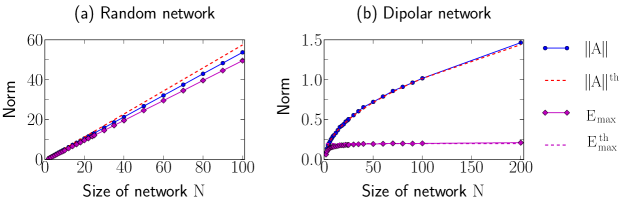
Figure 8: (Color online) Figure shows the scaling with network size $N$ of the matrix norms and largest eigenmodes of the adjacency matrices corresponding to (a) a random network and (b) a dipolar random network. The solid lines are average values obtained from 100 manifestations of the networks. The dashed lines are theoretical results. For the dipolar network, the largest eigenmode $E_{\text{max}}$ approaches a constant $1.6/d^{3}$ (dashed magenta line).

C.5 Dipolar coupled regular network

Here we consider a regular, symmetric network in two or three dimensions. To a good approximation, we can assume,

$$\|A\|=n\|A\|_{\text{cell}}$$ (40)

where $\|A\|_{\text{cell}}$ is the adjacency matrix of the unit cell of the underlying lattice, and $n$ is the number of tilings of this unit cell,

$$n\approx\frac{N}{N_{\text{cell}}}$$ (41)

where $N_{\text{cell}}$ is the number of nodes per unit cell.

$\|A\|_{\text{cell}}$ depends on the choice of lattice in the particular network. Let us consider the case of a honeycomb lattice, where we assume only nearest neighbor interactions. This network is found naturally in graphene and CNTs. Then, $\|A\|_{\text{cell}}=24/d^{3}$. Hence, for graphene,

$$\|A\|=\frac{2\sqrt{N}}{d^{3}}$$ (42)

C.6 Dipolar coupled regular network with vacancies

Let the probability of a vacancy occurring be $p$. Once again we assume a binomial distribution. We also assume, that we can estimate the norm in this case by using tiling – i.e. we consider the vacancies only in the unit cells. Consider for simplicity the special case of graphene. For $j$ vacancies, we have,

$$P_{j}={}^{N_{\text{cell}}}C_{j}p^{j}(1-p)^{N_{\text{cell}}-j}$$ (43)

The corresponding adjacency matrix,

$$\|A\|_{j}=\frac{4N_{\text{cell}}-j}{d^{3}}$$ (44)

Hence the mean,

$$\|A\|_{\text{cell}}=\sum_{j}P_{j}\|A\|_{j}=\frac{4N_{\text{cell}}(1-p)}{d^{3}}$$ (45)

Hence,

$$\|A\|=\frac{2\sqrt{N(1-p)}}{d^{3}}$$ (46)

References

- Kimble (2008) H. J. Kimble, Nature 453, 1023 (2008).
- Cirac et al. (1997) J. I. Cirac, P. Zoller, H. J. Kimble, and H. Mabuchi, Phys. Rev. Lett. 78, 3221 (1997).
- Bose (2003) S. Bose, Phys. Rev. Lett. 91, 207901 (2003).
- Christandl et al. (2004) M. Christandl, N. Datta, A. Ekert, and A. J. Landahl, Phys. Rev. Lett. 92, 187902 (2004).
- Wojcik et al. (2005) A. Wojcik, T. Luczak, P. Kurzynski, A. Grudka, T. Gdala, and M. Bednarska, Phys. Rev. A 72, 034303 (2005).
- Li et al. (2005) Y. Li, T. Shi, B. Chen, Z. Song, and C.-P. Sun, Phys. Rev. A 71, 022301 (2005).
- Gualdi et al. (2008) G. Gualdi, V. Kostak, I. Marzoli, and P. Tombesi, Phys. Rev. A 78, 022325 (2008).
- Yao et al. (2011) N. Y. Yao, L. Jiang, A. V. Gorshkov, Z.-X. Gong, A. Zhai, L.-M. Duan, and M. D. Lukin, Phys. Rev. Lett. 106, 040505 (2011).
- Wójcik et al. (2007) A. Wójcik, T. Łuczak, P. Kurzyński, A. Grudka, T. Gdala, and M. Bednarska, Phys. Rev. A 75, 022330 (2007).
- Strauch and Williams (2008) F. W. Strauch and C. J. Williams, Phys. Rev. B 78, 094516 (2008).
- Hirjibehedin et al. (2006) C. F. Hirjibehedin, C. P. Lutz, and A. Heinrich, Science 312, 1021 (2006).
- Spinicelli et al. (2011) P. Spinicelli, A. Drau, L. Rondin, F. Silva, J. Achard, S. Xavier, S. Bansropun, T. Debuisschert, S. Pezzagna, J. Meijer, et al., New J. Phys. 13, 025014 (2011).
- Ajoy et al. (2012) A. Ajoy, R. K. Rao, A. Kumar, and P. Rungta, Phys. Rev. A 85, 030303 (2012).
- Banchi et al. (2011) L. Banchi, T. J. G. Apollaro, A. Cuccoli, R. Vaia, and P. Verrucchi, New Journal of Physics 13, 123006 (2011).
- Ajoy and Cappellaro (2012a) A. Ajoy and P. Cappellaro, Phys. Rev. A 85, 042305 (2012a).
- Dutt et al. (2007) M. V. G. Dutt, L. Childress, L. Jiang, E. Togan, J. Maze, F. Jelezko, A. S. Zibrov, P. R. Hemmer, and M. D. Lukin, Science 316, 1312 (2007).
- Jelezko and Wrachtrup (2006) F. Jelezko and J. Wrachtrup, Physica Status Solidi (A) 203, 3207 (2006).
- Barklie and Guven (1981) R. C. Barklie and J. Guven, Journal of Physics C: Solid State Physics 14, 3621 (1981).
- Hanson et al. (2008) R. Hanson, V. V. Dobrovitski, A. E. Feiguin, O. Gywat, and D. D. Awschalom, Science 320, 352 (2008).
- Cappellaro et al. (2011) P. Cappellaro, L. Viola, and C. Ramanathan, Phys. Rev. A 83, 032304 (2011).
- Yao et al. (2012) N. Yao, L. Jiang, A. Gorshkov, P. Maurer, G. Giedke, J. Cirac, and M. Lukin, Nat Commun 3, 800 (2012).
- Cappellaro et al. (2007) P. Cappellaro, C. Ramanathan, and D. G. Cory, Phys. Rev. Lett. 99, 250506 (2007).
- Benjamin and Bose (2003) S. C. Benjamin and S. Bose, Phys. Rev. Lett. 90, 247901 (2003).
- Bhatia (1996) R. Bhatia, Matrix Analysis (Springer, 1996).
- Ajoy et al. (2011) A. Ajoy, G. A. Álvarez, and D. Suter, Phys. Rev. A 83, 032303 (2011).
- Levitt (2008) M. H. Levitt, J. Chem. Phys. 128, 052205 (2008).
- Suzuki (1990) M. Suzuki, Phys. Lett. A 146, 319 (1990).
- Cohen-Tannoudji et al. (1992) C. Cohen-Tannoudji, J. Dupont-Roc, and G. Grynberg, Atom-Photon Interactions: Basic Processes and Applications (Wiley-Interscience, 1992).
- Haus and Huang (1991) H. Haus and W. Huang, Proceedings of the IEEE 79, 1505 (1991).
- Synder and Love (1983) A. Synder and J. Love, Optical Waveguide Theory (Springer, 1983).
- Schrieffer and Wolff (1966) J. R. Schrieffer and P. A. Wolff, Phys. Rev. 149, 491 (1966).
- Bravyi et al. (2011) S. Bravyi, D. DiVincenzo, and D. Loss, Ann. Phys. 326, 2793 (2011).
- Hartman and Hahn (1962) S. R. Hartman and E. L. Hahn, Phys. Rev. 128, 2042 (1962).
- (34) See supplementary online material.
- Trotter (1959) H. F. Trotter, Proc. Amer. Math. Soc. 10, 545 (1959).
- Braunschweiler and Ernst (1983) L. Braunschweiler and R. R. Ernst, J. Magn. Reson. 53, 521 (1983).
- Balasubramanian et al. (2009) G. Balasubramanian, P. Neumann, D. Twitchen, M. Markham, R. Kolesov, N. Mizuochi, J. Isoya, J. Achard, J. Beck, J. Tissler, et al., Nat Mater 8, 383 (2009).
- Stanwix et al. (2010) P. L. Stanwix, L. M. Pham, J. R. Maze, D. L. Sage, T. K. Yeung, P. Cappellaro, P. R. Hemmer, A. Yacoby, M. D. Lukin, and R. L. Walsworth, Phys. Rev. B 82, 201201 (2010).
- Ajoy and Cappellaro (2012b) A. Ajoy and P. Cappellaro, unpublished (2012b).