Formulas for Lyapunov Exponents

Abstract.

We derive a series summation formula for the average logarithm norm of the action of a matrix on the projective space. This formula is shown to be useful to evaluate some Lyapunov exponents of random ${\rm SL}$-matrix cocycles, which include a special class for which H. Furstenberg had provided an explicit integral formula.

1. Introduction

Lyapunov exponents measure the rate of separation of nearby orbits in a given dynamical system. Linear cocycles form a class of dynamical systems where the study of Lyapunov exponents is an important and active subject. Roughly, a linear cocycle is a dynamical system on a vector bundle which acts linearly on fibers, over some fixed dynamics on the base of the vector bundle. In this article we shall deal with a special class of linear cocycles where the base dynamics is a Bernoulli shift equipped with a (constant factor) product measure, and the fiber is the special linear group ${\rm SL}(d,\mathbb{R})$. These cocycles, that we will refer as ‘random linear cocycles’, were extensively studied by H. Furstenberg. See [9], [10], [11],  [12]. More precisely, if $G$ is some matrix Lie group, like ${\rm SL}(d,\mathbb{R})$, a random linear cocycle is determined by a probability measure $\mu$ on $G$ together with a map $F:G^{\mathbb{N}}\times\mathbb{R}^{d}\to G^{\mathbb{N}}\times\mathbb{R}^{d}$ defined by $F(\underline{g},v)=(\sigma(\underline{g}),g_{0}\,v)$, where $\underline{g}$ denotes a matrix sequence $\{g_{n}\}_{n\in\mathbb{N}}$ and $\sigma:G^{\mathbb{N}}\to G^{\mathbb{N}}$ denotes the shift map   $\sigma\{g_{n}\}_{n\in\mathbb{N}}=\{g_{n+1}\}_{n\in\mathbb{N}}$. The measure $\mu$ on $G$ determines the product Bernoulli measure $\underline{\mu}=\mu^{\mathbb{N}}$ on the bundle’s base $G^{\mathbb{N}}$, which is shift invariant. It is always assumed in this theory that $\mu$ is ‘integrable’, which means that $\int_{G}\log^{+}\left\|g\right\|\,d\mu(g)<+\infty$. The iterates of $F$ are given explicitly by $F^{n}(\underline{g},v)=(\sigma^{n}\underline{g},g_{n-1}\,\ldots\,g_{1}\,g_{0}\,v)$. From a probabilistic point of view, this random cocycle is determined by the independent and identically distributed random process $X_{n}:G^{\mathbb{N}}\to G$, defined by $X_{n}(\underline{g})=g_{n}=X_{0}(\sigma^{n}\underline{g})$. Furstenberg and Kesten [11] have proven that the following limit, expressing the growth rate of the product random process $Y_{n}=X_{n-1}\,\ldots\,X_{1}\,X_{0}$, always exists and is constant for $\underline{\mu}$-almost every $\underline{g}\in G^{\mathbb{N}}$,

$$\lambda(\mu)=\lim_{n\to+\infty}\frac{1}{n}\,\log\left\|g_{n-1}\,\ldots\,g_{1}\,g_{0}\right\|=\lim_{n\to+\infty}\frac{1}{n}\,\log\left\|Y_{n}(\underline{g})\right\|\;.$$

The average growth rate $\lambda(\mu)$ relates to the Lyapunov exponent as follows. Given $(\underline{g},v)\in G^{\mathbb{N}}\times\mathbb{R}^{d}$, the Lyapunov exponent at $\underline{g}$ along $v$ is the limit

$$\lambda_{\mu}(v)=\lim_{n\to+\infty}\frac{1}{n}\,\log\left\|g_{n-1}\,\ldots\,g_{1}\,g_{0}\,v\right\|=\lim_{n\to+\infty}\frac{1}{n}\,\log\left\|Y_{n}(\underline{g})\,v\right\|\;,$$

which exists for every $v\in\mathbb{R}^{d}-\{0\}$ and $\underline{\mu}$-almost every $\underline{g}\in G^{\mathbb{N}}$. Moreover, this limit is constant $\underline{\mu}$-almost everywhere and $\lambda_{\mu}(v)\leq\lambda(\mu)$ for every $v\in\mathbb{R}^{d}-\{0\}$, with equality for almost every $v\in\mathbb{R}^{d}$. In fact, strict inequality can only occur for vectors in some $\mu$-invariant proper vector subspace $V\subset\mathbb{R}^{d}$, i.e., one which is invariant under all matrices $g$ in the support of $\mu$. See theorem 3.5 of [12]. This shows that $\lambda(\mu)$ is the largest Lyapunov exponent of the random cocycle. Furstenberg and Kifer give a nice variational characterization of all the Lyapunov spectra in [12], but we shall only deal with the largest Lyapunov exponent $\lambda(\mu)$ here. In [10] H. Furstenberg established the following integral formula for the Lyapunov exponent

$$\lambda(\mu)=\int_{{\rm SL}(d,\mathbb{R})}\int_{\mathbb{P}^{d-1}}\log\left\|g\,x\right\|\,d\nu(x)\,d\mu(g)\;,$$ (1.1)

where $\mathbb{P}^{d-1}$ denotes the projective space of lines in $\mathbb{R}^{d}$, and $\nu$ stands for any maximal $\mu$-stationary measure. A measure $\nu$ on $\mathbb{P}^{d-1}$ is said to be $\mu$-stationary   iff  $\mu\times\nu$ is an $F$-invariant measure. This amounts to say that $\nu$ is a fixed point of the convolution operator $P_{\mu}(\nu)=\mu\ast\nu=\int g_{\ast}\nu\,d\mu(g)$, induced by $\mu$ on the space of Borel probability measures on $\mathbb{P}^{d-1}$. A $\mu$-stationary measure is said to be maximal if it maximizes the left-hand-side integral in (1.1). See for instance section 3 of [12] for proofs of these facts. Furstenberg also found very general sufficient conditions for the largest Lyapunov exponent to be strictly positive. It is enough that the group $G$ generated by the support of $\mu$ is non compact, and no subgroup of $G$ with finite index is reducible. A group $G$ generated by matrices in the support of $\mu$ is said to be reducible   iff  there is a non trivial decomposition of $\mathbb{R}^{d}$ as a direct sum of $\mu$-invariant subspaces of $\mathbb{R}^{d}$. See theorem 8.6 in [10].

Furstenberg’s formula (1.1) indicates a way of computing Lyapunov exponents. But still a couple of problems persists.

1. To determine the $\mu$-stationary measures explicitly.

2. To compute the following integral numerically

   $$R_{\nu}(g)=\int_{\mathbb{P}^{d-1}}\log\left\|g\,x\right\|\,d\nu(x)\;.$$ (1.2)

In [10] Furstenberg solves the first problem for a special class of measures on ${\rm SL}(d,\mathbb{R})$. See theorem 7.3 of [10]. In this paper we address the second problem mainly. First we consider the uniform Riemannian probability measure $m$ on $\mathbb{P}^{d-1}$ and prove in section 3 that

Theorem A  Given $g\in{\rm SL}(d,\mathbb{R})$ with singular values $0<\lambda_{1}\leq\lambda_{2}\leq\ldots\,\lambda_{d}$, if $\lambda_{\ast}>\lambda_{d}/\sqrt{2}$ then the following series converges absolutely

$$R_{m}(g)=\log\lambda_{\ast}-\sum_{r=1}^{\infty}\frac{1}{2\,r}\,\sum_{r_{1}+\cdots+r_{d}=r}\Theta^{(d)}_{r_{1},\ldots,r_{d}}\,\left(1-\frac{\lambda_{1}^{2}}{\lambda_{\ast}^{2}}\right)^{r_{1}}\,\ldots\,\left(1-\frac{\lambda_{d}^{2}}{\lambda_{\ast}^{2}}\right)^{r_{d}}\;,$$

where

$$\Theta^{\,(d)}_{r_{1},\ldots,r_{d}}=\frac{r!}{r_{1}!\cdots r_{d}!}\,\frac{(2r_{1}-1)!!\cdots(2r_{d}-1)!!}{d(d+2)\cdots(d+2r-2)}\;.$$ (1.3)

Moreover, the coefficients $\Theta^{\,(d)}_{r_{1},\ldots,r_{d}}$ form a permutation invariant probability distribution on the finite set  $\mathscr{I}_{r}=\{\,(r_{1},\ldots,r_{d})\in\mathbb{N}^{d}\,:\,r_{1}+\ldots+r_{d}=r\,\}$.

In the last section 4, we provide some applications of Theorem A. First, we give an explicit formula for the largest Lyapunov exponent of the random cocycles where Furstenberg was able to give explicit stationary measures. This formula is given in terms of the integrals $R_{m}(g)$, to which we can apply Theorem A above. In a few special cases, these formulas are used in numerical computations of some Lyapunov exponents. A second motivation for proving Theorem A was the role played by the integral $R_{m}(g)$ in the following conjecture. For any dimension $d>2$ and every $g\in{\rm SL}(d,\mathbb{R})$,

$$\int_{{\rm SO}(d)}\log\rho(k\,g)\,dk\geq R_{m}(g),$$ (1.4)

where $\rho$ stands for the spectral radius and $dk$ represents integration with respect to the normalized Haar measure in the special orthogonal group ${\rm SO}(d)$. This is conjectured in [7, Question 6.6]. An analogous result is proved in [8] for the unitary group in ${\rm GL}(d,\mathbb{C})$. Theorem A is based on the following more general result, to be proved in section 2.

Theorem B  Given a probability measure $\nu\in\mathscr{P}(\mathbb{P}^{d-1})$, and $g\in{\rm SL}(d,\mathbb{R})$ with singular values $0<\lambda_{1}\leq\lambda_{2}\leq\ldots\,\lambda_{d}$, if $\lambda_{\ast}>\lambda_{d}/\sqrt{2}$ then the following series converges absolutely

$$R_{\nu}(g)=\log\lambda_{\ast}-\sum_{r=1}^{\infty}\frac{1}{2\,r}\,\sum_{r_{1}+\cdots+r_{d}=r}\Theta^{(d)}_{r_{1},\ldots,r_{d}}(k,\nu)\,\left(1-\frac{\lambda_{1}^{2}}{\lambda_{\ast}^{2}}\right)^{r_{1}}\,\ldots\,\left(1-\frac{\lambda_{d}^{2}}{\lambda_{\ast}^{2}}\right)^{r_{d}}\;,$$

where

$$\Theta^{\,(d)}_{r_{1},\ldots,r_{d}}(k,\nu)=\frac{r!}{r_{1}!\cdots r_{d}!}\,\int_{\mathbb{P}^{d-1}}Q_{r_{1},\ldots,r_{d}}(k\,x)\,d\nu(x)\;,$$

$Q_{r_{1},\ldots,r_{d}}:\mathbb{P}^{d-1}\to\mathbb{R}$  stands for the function  $Q_{r_{1},\ldots,r_{d}}(x_{1},\ldots,x_{d})=x_{1}^{2\,r_{1}}\,\ldots\,x_{1}^{2\,r_{d}}$, and $k\in{\rm O}(d,\mathbb{R})$ is an orthogonal matrix such that $kg^{T}gk^{-1}$ is a diagonal.
Moreover, the coefficients $\Theta^{\,(d)}_{r_{1},\ldots,r_{d}}(k,\nu)$ form a probability distribution on the finite set  $\mathscr{I}_{r}=\{\,(r_{1},\ldots,r_{d})\in\mathbb{N}^{d}\,:\,r_{1}+\ldots+r_{d}=r\,\}$.

Let us remark that in theorem A the coefficients $\Theta^{\,(d)}_{r_{1},\ldots,r_{d}}$:

1. are given explicitly,

2. do not depend on the singular value decomposition of $g$, and

3. are invariant under permutations of the indices $(r_{1},\ldots,r_{d})$.

Although more general, all these properties fail in theorem B.

Defining $\Theta^{\,(d)}_{r_{1},\ldots,r_{d}}(\nu):=\Theta^{\,(d)}_{r_{1},\ldots,r_{d}}(id,\nu)$, we have $\Theta^{\,(d)}_{r_{1},\ldots,r_{d}}(k,\nu)=\Theta^{\,(d)}_{r_{1},\ldots,r_{d}}(k\,\nu)$, and the measure $\widetilde{\nu}=k\nu$ is $\widetilde{\mu}$-stationary with $\widetilde{\mu}=k\mu k^{-1}$. Hence, there is no loss of generality in assuming that $k=id$, i.e., $g$ is a diagonal matrix, in theorem B.

If we have upper bounds on some of the coefficients $\Theta^{\,(d)}_{r_{1},\ldots,r_{d}}(k\nu)$ then we can use theorem B to obtain a corresponding lower bound for $R_{\nu}(g)$. For instance, in proposition 2 we shall derive the following universal upper bound

$$\sum_{r_{1}+\cdots+r_{d}=r}\Theta_{r_{1},\ldots,r_{d}}(k,\nu)\,\left(1-\frac{\lambda_{1}^{2}}{\lambda_{\ast}^{2}}\right)^{r_{1}}\,\ldots\,\left(1-\frac{\lambda_{d}^{2}}{\lambda_{\ast}^{2}}\right)^{r_{d}}\leq\left(1-\frac{\lambda_{1}^{2}}{\lambda_{\ast}^{2}}\right)^{r}\;.$$

Then, combining this with theorem B, we can derive the trivial lower bound $R_{\nu}(g)\geq\log\lambda_{1}$, where $\lambda_{1}$ denotes the least singular value of $g$.

The family of functions $Q_{r_{1},\ldots,r_{d}}:\mathbb{P}^{d-1}\to\mathbb{R}$, with $(r_{1},\ldots,r_{d})\in\mathbb{N}^{d}$, separates points in $\mathbb{P}^{d-1}$. Hence, by Stone-Weirestrass’ theorem, the linear space spanned by these monomials is a dense subalgebra of $\mathscr{C}(\mathbb{P}^{d-1})$. In particular, the measure $\nu$ is completely determined by the ‘momenta’ $\Theta_{r_{1},\ldots,r_{d}}(\nu)$. If we could devise some convergent iterative scheme to approximate these ‘$\mu$-stationary momenta’, instead of the $\mu$-stationary measure $\nu$, then we would apply theorem B and get bounds on the Lyapounov exponent $R_{\nu}(g)$.

2. A General Formula

Given integers $r_{1}\geq 0,\,\ldots,\,r_{d}\geq 0$, consider the function $Q_{r_{1},\ldots,r_{d}}:\mathbb{P}^{d-1}\to\mathbb{R}$

$$Q_{r_{1},\ldots,r_{d}}(x_{1},\ldots,x_{d})=x_{1}^{2\,r_{1}}\ldots x_{d}^{2\,r_{d}}\;.$$ (2.1)

This is a bounded function taking values between $0$ and $1$. Setting $r=r_{1}+\ldots+r_{d}$, the minimum value of $Q_{r_{1},\ldots,r_{d}}$ is $0$ while the maximum value, $(r_{1}/r)^{r_{1}}\,\ldots\,(r_{d}/r)^{r_{d}}$, is attained at the projective points with coordinates $\left(\pm\sqrt{r_{1}/r},\ldots,\pm\sqrt{r_{d}/r}\right)$. Let $\mathscr{P}(\mathbb{P}^{d-1})$ denote the space of Borel probability measures on $\mathbb{P}^{d-1}$. Throughout this section, $\nu$ will denote any probability measure in $\mathscr{P}(\mathbb{P}^{d-1})$.

Proposition 1.

Let $A\in{\rm gl}(d,\mathbb{R})$ be a symmetric matrix of the form $A=k^{-1}\,D\,k$, where $k^{-1}$ is an orthogonal matrix consisting of $A$’s eigenvectors and $D={\rm diag}(\lambda_{1},\ldots,\lambda_{d})$ is the corresponding eigenvalue matrix. Then

$$\int_{\mathbb{P}^{d-1}}\langle A\,x,x\rangle^{r}\,d\nu(x)=\sum_{r_{1}+\cdots+r_{d}=r}\Theta^{\,(d)}_{r_{1},\ldots,r_{d}}(k,\nu)\,\lambda_{1}^{r_{1}}\ldots\lambda_{d}^{r_{d}}\;,$$ (2.2)

where

$$\Theta^{\,(d)}_{r_{1},\ldots,r_{d}}(k,\nu)=\frac{r!}{r_{1}!\cdots r_{d}!}\,\int_{\mathbb{P}^{d-1}}Q_{r_{1},\ldots,r_{d}}(k\,x)\,d\nu(x)\;.$$ (2.3)

Proof.  Using the multinomial formula we get

$$\int_{\mathbb{P}^{d-1}}\left(\sum_{i=1}^{d}\lambda_{i}\,x_{i}^{2}\right)^{r}\,d\nu(x_{1},\ldots,x_{d})=\sum_{r_{1}+\cdots+r_{d}=r}\frac{r!}{r_{1}!\ldots r_{d}!}\,\left(\int_{\mathbb{P}^{d-1}}Q_{r_{1},\ldots,r_{q}}\,d\nu\right)\,\lambda_{1}^{r_{1}}\ldots\lambda_{d}^{r_{d}}\;,$$

which is the stated formula with $A=D={\rm diag}(\lambda_{1},\ldots,\lambda_{d})$. The general case follows in the same way but replacing $x$ by $k\,x$ before integrating with respect to $\nu$. Note that $\langle A\,x,x\rangle=\sum_{i=1}^{d}\lambda_{i}\,(k_{i}\,x)^{2}$ with $k\,x=(k_{1}\,x,\ldots,k_{d}\,x)$. $\sqcup\!\!\!\!\sqcap\vskip 12.0pt plus 4.0pt minus 4.0pt$

Given a probability measure $\nu\in\mathscr{P}(\mathbb{P}^{d-1})$, and integers $r_{1}\geq 0,\,\ldots,\,r_{d}\geq 0$ we shall denote the matrix function defined in (2.3) by   $\Theta^{\nu}_{r_{1},\ldots,r_{d}}:{\rm O}(d,\mathbb{R})\to\mathbb{R}$.

Corollary 1.

$\{\Theta^{\nu}_{r_{1},\ldots,r_{d}}\}$ is a family of non-negative bounded functions such that

$$\sum_{r_{1}+\cdots+r_{d}=r}\Theta^{\nu}_{r_{1},\ldots,r_{d}}(k)=1\quad\text{ for every matrix }\;k\in{\rm O}(d,\mathbb{R})\;.$$

Proof.  First

$$0<\Theta^{\nu}_{r_{1},\ldots,r_{d}}\leq\frac{r!}{r_{1}!\ldots r_{d}!}\,(r_{1}/r)^{r_{1}}\,\ldots\,(r_{d}/r)^{r_{d}}=\frac{r!}{r^{r}}\,\frac{r_{1}^{r_{1}}}{r_{1}!}\,\ldots\,\frac{r_{d}^{r_{d}}}{r_{d}!}$$

because $0<Q_{r_{1},\ldots,r_{d}}\leq(r_{1}/r)^{r_{1}}\,\ldots\,(r_{d}/r)^{r_{d}}$. By proposition 1,

$$\sum_{r_{1}+\cdots+r_{d}=r}\Theta^{\nu}_{r_{1},\ldots,r_{d}}(k) =\sum_{r_{1}+\cdots+r_{d}=r}\int_{\mathbb{P}^{d-1}}\frac{r!}{r_{1}!\,\ldots\,r_{d}!}\,Q_{r_{1},\ldots,r_{d}}(k\,x)\,d\nu(x)$$

$$=\sum_{r_{1}+\cdots+r_{d}=r}\int_{\mathbb{P}^{d-1}}\frac{r!}{r_{1}!\,\ldots\,r_{d}!}\,Q_{r_{1},\ldots,r_{d}}(x)\,dk_{\ast}\nu(x)$$

$$=\int_{\mathbb{P}^{d-1}}\langle x,x\rangle^{r}\,dk_{\ast}\nu(x)=1\;.$$

$\sqcup\!\!\!\!\sqcap\vskip 12.0pt plus 4.0pt minus 4.0pt$

Proof of theorem B.   We use the following Taylor’ series for the logarithm function

$$\log x=\log x_{0}-\sum_{r=1}^{\infty}\frac{1}{r}\,\left(1-x_{0}^{-1}\,x\right)^{r}\;.$$

Take $x_{0}=\lambda_{\ast}^{2}$   and   $b=I-\lambda_{\ast}^{-2}\,g^{T}g$.   Note that   $\lambda_{\ast}^{-2}\,\left\|g\,x\right\|^{2}=\langle\lambda_{\ast}^{-2}\,g^{T}g\,x,x\rangle$   and $b=k^{-1}\,{\rm diag}\left(1-\frac{\lambda_{1}^{2}}{\lambda_{\ast}^{2}},\ldots,1-\frac{\lambda_{d}^{2}}{\lambda_{\ast}^{2}}\right)\,k$. Hence, by proposition 1,

$$\int_{\mathbb{P}^{d-1}}\log\left\|g\,x\right\|\,d\nu(x) =\frac{1}{2}\,\int_{\mathbb{P}^{d-1}}\log\left\|g\,x\right\|^{2}\,d\nu(x)$$

$$=\log\lambda_{\ast}-\sum_{r=1}^{\infty}\frac{1}{2\,r}\,\int_{\mathbb{P}^{d-1}}\left(1-\lambda_{\ast}^{-2}\,\left\|g\,x\right\|^{2}\right)^{r}\,d\nu(x)$$

$$=\log\lambda_{\ast}-\sum_{r=1}^{\infty}\frac{1}{2\,r}\,\int_{\mathbb{P}^{d-1}}\langle b\,x,x\rangle^{r}\,d\nu(x)$$

$$=\log\lambda_{\ast}-\sum_{r=1}^{\infty}\frac{1}{2\,r}\,\sum_{r_{1}+\cdots+r_{d}=r}\Theta^{(d)}_{r_{1},\ldots,r_{d}}(k,\nu)\,\left(1-\frac{\lambda_{1}^{2}}{\lambda_{\ast}^{2}}\right)^{r_{1}}\,\ldots\,\left(1-\frac{\lambda_{d}^{2}}{\lambda_{\ast}^{2}}\right)^{r_{d}}\;.$$

The assumption $\lambda_{\ast}>\lambda_{d}/\sqrt{2}$ implies that

$$\alpha=\max_{1\leq i\leq d}\left|{1-\frac{\lambda_{i}^{2}}{\lambda_{\ast}^{2}}}\right|<1\;.$$

The r.h.s. converges absolutely because the absolute value series is majorated by

$$\sum_{r=1}^{\infty}\frac{1}{2\,r}\,\sum_{r_{1}+\cdots+r_{d}=r}\Theta^{(d)}_{r_{1},\ldots,r_{d}}(k,\nu)\,\alpha^{r}=\sum_{r=1}^{\infty}\frac{\alpha^{r}}{2\,r}<+\infty\;.$$

∎

Remark 1.

Assuming $\lambda_{\ast}>\sqrt{(\lambda_{1}^{2}+\lambda_{d}^{2})/2}$ we have

$$\alpha=\max_{1\leq i\leq d}\left(1-\frac{\lambda_{i}^{2}}{\lambda_{\ast}^{2}}\right)=1-\frac{\lambda_{1}^{2}}{\lambda_{\ast}^{2}}\;\in(0,1)\;.$$

We end this section with one more remark.

Proposition 2.

Given $g\in{\rm SL}(d,\mathbb{R})$ with singular values $0<\lambda_{1}\leq\ldots\leq\lambda_{d}$, let $k$ be an orthogonal matrix such that $g^{T}g=k^{-1}\,{\rm diag}(\lambda_{1}^{2},\ldots,\lambda_{d}^{2})\,k$. If $\lambda_{\ast}>\sqrt{(\lambda_{1}^{2}+\lambda_{d}^{2})/2}$ then

$$\sum_{r_{1}+\cdots+r_{d}=r}\Theta^{(d)}_{r_{1},\ldots,r_{d}}(k,\nu)\,\left(1-\frac{\lambda_{1}^{2}}{\lambda_{\ast}^{2}}\right)^{r_{1}}\,\ldots\,\left(1-\frac{\lambda_{d}^{2}}{\lambda_{\ast}^{2}}\right)^{r_{d}}\leq\left(1-\frac{\lambda_{1}^{2}}{\lambda_{\ast}^{2}}\right)^{r}\;.$$

Proof.  Combine corollary 1 with remark 1. $\sqcup\!\!\!\!\sqcap\vskip 12.0pt plus 4.0pt minus 4.0pt$

3. Spherical Integrals

Theorem A follows from theorem B using next formula.

Proposition 3.

Given integers $r_{1}\geq 0,\,\ldots,\,r_{d}\geq 0$,

$$\int_{\mathbb{P}^{d-1}}Q_{r_{1},\ldots,r_{d}}\,dm=\frac{(2\,r_{1}-1)!!\ldots(2\,r_{d}-1)!!}{d\,(d+2)\,\ldots\,(d+2r-2)}\;.$$ (3.1)

This formula involves the concept of double factorial, which relates with Euler’s Gamma function. The double factorial is the recursive function defined over the natural numbers by the relation $n!!=n\,(n-2)!!$ with initial conditions $0!!=(-1)!!=1$. The Gamma function, defined by the improper integral

$$\Gamma(x)=\int_{0}^{\infty}t^{x-1}\,e^{-t}\,dt\quad(x>0)\;,$$

is a solution of the functional equation

$$\Gamma(x+1)=x\,\Gamma(x)\;.$$ (3.2)

Since $\Gamma(1)=\int_{0}^{\infty}e^{-t}\,dt=1$   it follows at once that $\Gamma(n)=(n-1)!$ for every $n\in\mathbb{N}$. In other words, the Gamma function is a real analytic interpolation of the usual factorial function over the natural numbers. Likewise, because $\Gamma(1/2)=\sqrt{2}$ it follows easily by induction that for every $n\in\mathbb{N}$,

$$\Gamma\left(n+\frac{1}{2}\right)=\frac{(2n-1)!!}{2^{n}}\,\sqrt{\pi}\;.$$ (3.3)

We refer [2] for a comprehensive treatment on the Gamma function. See formula (1.1.22) there for a justification of the value $\Gamma(1/2)=\sqrt{2}$.

The Gamma function can be used to provide explicit formulas for the volumes of spheres and balls. Let $\mathbb{D}^{d}=\{\,x\in\mathbb{R}^{d}\,:\,\left\|x\right\|^{2}\leq 1\,\}$ be the Euclidean unit disk and denote its volume by ${\rm V}_{d}$. As above, let $\mathbb{S}^{d-1}$ be the Euclidean unit sphere, i.e., the boundary of $\mathbb{D}^{d}$, and denote its area by ${\rm A}_{d-1}=\int_{\mathbb{S}^{d-1}}1\,d\sigma$, where $\sigma$ stands for the measure induced by the canonical Euclidean induced metric on $\mathbb{S}^{d-1}$. The Divergence theorem, together with a simple change of variables, may be used to establish the following recursive relations between these volumes (see appendix A of [5])

$${\rm V}_{d}=\frac{2\,\pi}{d}\,{\rm V}_{d-2}\quad\text{ and }\quad{\rm A}_{d-1}=d\,{\rm V}_{d}\;.$$ (3.4)

From these relations we deduce explicit formulas for the volumes of balls and spheres:

$${\rm V}_{d}=\frac{\pi^{d/2}}{\Gamma(1+d/2)}\quad\text{ and }\quad{\rm A}_{d-1}=2\,\frac{\pi^{d/2}}{\Gamma(d/2)}\;.$$ (3.5)

To see this set ${\rm U}_{d}={\pi^{d/2}}/{\Gamma(1+d/2)}$. The functional equation (3.2) implies that ${\rm U}_{d}$ satisfies the same recursive equation as ${\rm V}_{d}$,

$${\rm U}_{d}=\frac{\pi^{d/2}}{\Gamma(1+d/2)}=\frac{\pi}{d/2}\,\frac{\pi^{(d-2)/2}}{\Gamma(1+(d-2)/2)}=\frac{2\,\pi}{d}\,{\rm U}_{d-2}\;.$$

But since $\Gamma(1/2)=\sqrt{2}$, it follows that ${\rm U}_{1}=2={\rm V}_{1}$. Also ${\rm U}_{0}=1={\rm V}_{0}$. Hence the equality ${\rm V}_{d}={\rm U}_{d}$ holds for all $d\geq 0$. Finally, by (3.4) we get

$${\rm A}_{d-1}=d\,{\rm V}_{d}=d\,\frac{\pi^{d/2}}{\Gamma(1+d/2)}=2\,\frac{\pi^{d/2}}{\Gamma(d/2)}\;.$$

Proof of proposition 3.   We are going to reduce the integrals (3.1) to the following family of integrals introduced in [6]

$$I_{d}(r_{1},\ldots,r_{d})=\int_{\mathbb{D}^{d}}x_{1}^{2\,r_{1}}\ldots x_{d}^{2\,r_{d}}\,dx_{1}\,\ldots\,dx_{d}\;.$$

Using the Divergence Theorem the author deduces a recurrence formula from which he gets the following explicit formula for every $d\geq 2$, and every $r_{1}\geq 0,\,\ldots,\,r_{d}\geq 0$,

$$I_{d}(r_{1},\ldots,r_{d})=\frac{\Gamma(r_{1}+\frac{1}{2})\,\ldots\,\Gamma(r_{d}+\frac{1}{2})}{\Gamma(r_{1}+\cdots+r_{d}+1+\frac{d}{2})}\;.$$ (3.6)

Check formula (8) of [6]. It is also easy to see with a change of variables’ argument that for any $r$-homogeneous function $f:\mathbb{R}^{d}\to\mathbb{R}$ (see Corollary 1 of [6]),

$$\int_{\mathbb{D}^{d}}f(x_{1},\ldots,x_{d})\,dx_{1}\,\ldots\,dx_{d}=\frac{1}{d+r}\,\int_{\mathbb{S}^{d-1}}f(x_{1},\ldots,x_{d})\,d\sigma(x_{1},\ldots,x_{d})\;.$$ (3.7)

Now, combining (3.7), (3.6), (3.5) and (3.3) we get

$$\int_{\mathbb{P}^{d-1}}Q_{r_{1},\ldots,r_{d}}\,dm =\int_{\mathbb{S}^{d-1}}x_{1}^{2\,r_{1}}\ldots x_{d}^{2\,r_{d}}\,dm(x_{1},\ldots,x_{d})$$

$$=\frac{1}{{\rm A}_{d-1}}\,\int_{\mathbb{S}^{d-1}}x_{1}^{2\,r_{1}}\ldots x_{d}^{2\,r_{d}}\,d\sigma(x_{1},\ldots,x_{d})$$

$$=\frac{d+2\,r}{{\rm A}_{d-1}}\,I_{d}(r_{1},\ldots,r_{d})$$

$$=\frac{d+2\,r}{2\,\frac{\pi^{d/2}}{\Gamma(d/2)}}\,\frac{\Gamma(r_{1}+\frac{1}{2})\,\ldots\,\Gamma(r_{d}+\frac{1}{2})}{\Gamma(r+1+\frac{d}{2})}$$

$$=\frac{d+2\,r}{2^{r+1}}\,\frac{(2\,r_{1}-1)!!\,\ldots\,(2\,r_{d}-1)!!}{(r+\frac{d}{2})\,(r-1+\frac{d}{2})\,\ldots\,\frac{d}{2}}$$

$$=\frac{(2\,r_{1}-1)!!\ldots(2\,r_{d}-1)!!}{d\,(d+2)\,\ldots\,(d+2r-2)}$$

$\sqcup\!\!\!\!\sqcap\vskip 12.0pt plus 4.0pt minus 4.0pt$

Proof of theorem A.   In view of theorem B we just have to compute:

$$Q^{(d)}_{r_{1},\ldots,r_{d}}(k,m) =\frac{r!}{r_{1}!\ldots r_{d}!}\,\int_{\mathbb{P}^{d-1}}Q_{r_{1},\ldots,r_{d}}(k\,x)\,dm(x)$$

$$=\frac{r!}{r_{1}!\ldots r_{d}!}\,\int_{\mathbb{P}^{d-1}}Q_{r_{1},\ldots,r_{d}}(x)\,dk_{\ast}m(x)=\frac{r!}{r_{1}!\ldots r_{d}!}\,\int_{\mathbb{P}^{d-1}}Q_{r_{1},\ldots,r_{d}}\,dm\;,$$

the last equality because $k_{\ast}m=m$, for every orthogonal matrix $k\in{\rm O}(d,\mathbb{R})$. Combining this computation with proposition 3 we obtain formula (1.3) in theorem A. The coefficients $\Theta^{(d)}_{r_{1},\ldots,r_{d}}$ are obviously positive rational numbers, which by corollary 1 form a probability distribution on the set $\mathscr{I}_{r}$. An inspection to formula (1.3) shows these coefficients are invariant under permutations, i.e., $\Theta^{(d)}_{r_{1},\ldots,r_{d}}=\Theta^{(d)}_{r_{\pi_{1}},\ldots,r_{\pi_{d}}}$, for every permutation $\pi$ of $\{1,\ldots,d\}$. $\sqcup\!\!\!\!\sqcap\vskip 12.0pt plus 4.0pt minus 4.0pt$

4. Some Applications

Denote by $\mathscr{M}_{m}$ the space of probability measures $\mu$ in ${\rm SL}(d,\mathbb{R})$ that have $m$ as $\mu$-stationary measure, i.e., $\mu\ast m=m$. The class $\mathscr{M}_{m}$ is closed under orthogonal averages, i.e., if $\mu\in\mathscr{M}_{m}$ then $\int_{{\rm SO}(d,\mathbb{R})}k_{\ast}\mu\,dm(k)\in\mathscr{M}$.

Proposition 4.

For any measure $\mu\in\mathscr{M}_{m}$, its Lyapunov exponent is

$$\lambda(\mu)=\int_{{\rm SL}(d,\mathbb{R})}R_{m}(g)\,d\mu(g)\;.$$

Proof.  Follows from Furstenberg integral formula (1.1). $\sqcup\!\!\!\!\sqcap\vskip 12.0pt plus 4.0pt minus 4.0pt$

Theorem A can then be used to approximate this Lyapunov exponent. A class of examples in $\mathscr{M}_{m}$ are the so called orthogonally invariant measures. A probability $\mu\in\mathscr{P}({\rm SL}(d,\mathbb{R}))$ is said to be orthogonally invariant if $k_{\ast}\mu=\mu$ for every orthogonal matrix $k\in{\rm SO}(d,\mathbb{R})$. We list some equivalent characterizations of orthogonally invariant measures.

Proposition 5.

Given a measure $\mu\in\mathscr{P}({\rm SL}(d,\mathbb{R}))$, the following are equivalent:

1. $\mu$ is orthogonally invariant,

2. $\mu\ast\delta_{p}=m$,   $\forall\,p\in\mathbb{P}^{d-1}$,

3. $\mu\ast\nu=m$,   $\forall\,\nu\in\mathscr{P}(\mathbb{P}^{d-1})$,

4. $\mu=m_{K}\ast\theta$, for some measure $\theta\in\mathscr{P}({\rm SL}(d,\mathbb{R}))$,

where $m_{K}$ stands for the normalized Haar measure on $K={\rm SO}(d,\mathbb{R})$.

Proof.  The proof is straightforward. $\sqcup\!\!\!\!\sqcap\vskip 12.0pt plus 4.0pt minus 4.0pt$

Given a matrix $g\in{\rm SL}(d,\mathbb{R})$, consider the measure

$$\mu=m_{K}\ast\delta_{g}=\int_{{\rm SO}(d,\mathbb{R})}\delta_{kg}\,dm_{K}(k)\;.$$ (4.1)

Proposition 6.

The measure  (4.1) is orthogonally invariant, and its Lyapunov exponent is $\lambda(\mu)=R_{m}(g)$.

Proof.  Since $\mu$ is orthogonally invariant we have $\mu\ast m=m$, and hence by proposition 4

$$\lambda(\mu)=\int_{{\rm SL}}R_{m}(g^{\prime})\,d\mu(^{\prime})=\int_{{\rm SO}}R_{m}(k\,g)\,dm_{K}(k)=R_{m}(g)\;,$$

because all matrices $k\,g$ have the same singular values. $\sqcup\!\!\!\!\sqcap\vskip 12.0pt plus 4.0pt minus 4.0pt$

Consider now the matrix family

$$g_{t}=\left(\begin{array}[]{cc}tI_{d}&0\\ 0&t^{-1}I_{d}\end{array}\right)\in{\rm SL}(2d,\mathbb{R})\quad(t\geq 1)\;,$$ (4.2)

where $I_{d}$ denotes the identity $d\times d$ matrix. Next proposition refers to the following orthogonally invariant measure  $\mu_{t}=m_{K}\ast\delta_{g_{t}}$.

Proposition 7.

For every $t>1$, the Lyapunov exponent of $\mu_{t}$ is

$$\lambda_{2d}(\mu_{t})=\log t-\sum_{r=1}^{\infty}\frac{1}{2r}\,\frac{d(d+2)\ldots(d+2r-2)}{(2d)(2d+2)\ldots(2d+2r-2)}\,\left(1-\frac{1}{t^{4}}\right)^{r}\;.$$

Proof.  By proposition  6,   $\lambda_{2d}(\mu_{t})=R_{m}(g_{t})$. Notice that matrix $g_{t}$ has $d$ singular values equal to $t>1$, and $d$ singular values equal to $1/t<1$. Thus, applying theorem A with $\lambda_{\ast}=t$

$$\lambda_{2d}(\mu_{t})=R_{m}(g_{t})=\log t-\sum_{r=1}^{\infty}\frac{1}{2r}\,\sum_{r_{1}+\ldots+r_{d}=r}\Theta^{(2d)}_{0,\ldots,0,r_{1},\ldots,r_{d}}\,\left(1-\frac{1}{t^{4}}\right)^{r}\;.$$

Notice that if $0+\ldots+0+r_{1}+\ldots+r_{d}=r$,

$$\Theta^{(2d)}_{0,\ldots,0,r_{1},\ldots,r_{d}} =\frac{r!}{r_{1}!\cdots r_{d}!}\,\frac{(2r_{1}-1)!!\cdots(2r_{k}-1)!!}{(2d)(2d+2)\cdots(2d+2r-2)}$$

$$=\Theta^{(d)}_{r_{1},\ldots,r_{d}}\,\frac{(2d)(2d+2)\cdots(2d+2r-2)}{d(d+2)\cdots(d+2r-2)}$$

Hence, because $\sum_{r_{1}+\ldots+r_{d}=r}\Theta^{(d)}_{r_{1},\ldots,r_{d}}=1$,

$$\sum_{r_{1}+\ldots+r_{d}=r}\Theta^{(2d)}_{0,\ldots,0,r_{1},\ldots,r_{d}}=\frac{(2d)(2d+2)\cdots(2d+2r-2)}{d(d+2)\cdots(d+2r-2)}\;,$$

and we get the given formula for $\lambda_{2d}(\mu_{t})$. $\sqcup\!\!\!\!\sqcap\vskip 12.0pt plus 4.0pt minus 4.0pt$

Corollary 2.

The function sequence $\lambda_{2d}(\mu_{t})$ increases with $d$, and for every $t\geq 1$

$$\lim_{d\to+\infty}\lambda_{2d}(\mu_{t})=\log t+\frac{1}{2}\,\log\left(\frac{1+t^{4}}{2\,t^{4}}\right)\;.$$

Proof.  Notice that

$$\frac{d(d+2)\ldots(d+2r-2)}{(2d)(2d+2)\ldots(2d+2r-2)}\geq\frac{1}{2^{r}}\;,$$

and the right hand side decreases to $2^{-r}$ as $d$ grows to $+\infty$. The series $\sum_{r=1}^{\infty}\frac{1}{2^{r+1}r}\,\left(1-\frac{1}{t^{4}}\right)^{r}$ converges absolutely and uniformly to the function

$$g(t)=\log t-\sum_{r=1}^{\infty}\frac{1}{2^{r+1}r}\,\left(1-\frac{1}{t^{4}}\right)^{r}\;.$$

Because this series is essentially a geometric one we can compute its sum explicitly

$$g(t)=\log t+\frac{1}{2}\,\log\left(\frac{1+t^{4}}{2\,t^{4}}\right)\;.$$

Then, by Lebesgue monotone convergence theorem   $\lim_{d\to\infty}\lambda_{2d}(\mu_{t})=g(t)$. $\sqcup\!\!\!\!\sqcap\vskip 12.0pt plus 4.0pt minus 4.0pt$

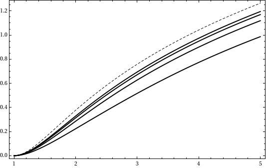
Figure 1. The graphs of $t\mapsto\lambda_{2d}(\mu_{t})$, for the half-dimensions $d=1,2,3,4$.

This corollary shows that for large dimensions, $\lambda_{2d}(\mu_{t})\approx\log t=\log\left\|g_{t}\right\|$, which is somehow expectable since all matrices in the support of $\mu_{t}$ have norm $t$.

The graphs of these functions, computed in Mathematica are depicted in figure 1. The dashed line represents the graph of $g(t)$.

For the following class of measures Furstenberg was able to give explicit stationary measures, see theorem 7.3 of [10]. Given two probability measures $\mu_{1}$ and $\mu_{2}$ in ${\rm SL}(d,\mathbb{R})$, define the measure

$$\mu=\mu_{1}\ast m_{K}\ast\mu_{2}=\int_{{\rm SL}}\int_{{\rm SO}}\int_{{\rm SL}}\delta_{g_{1}kg_{2}}\,d\mu_{1}(g_{1})\,dm_{K}(k)\,d\mu_{2}(g_{2})\;.$$ (4.3)

The $\mu$-stationary measure of $\mu$ is $\mu_{1}\ast m$. In fact, by item 4. of proposition 5, the measure $m_{K}\ast\mu_{2}\ast\mu_{1}$ is orthogonally invariant. Hence $(m_{K}\ast\mu_{2}\ast\mu_{1})\ast m=m$ and

$$\mu\ast(\mu_{1}\ast m) =(\mu_{1}\ast m_{K}\ast\mu_{2})\ast(\mu_{1}\ast m)$$

$$=\mu_{1}\ast(m_{K}\ast\mu_{2}\ast\mu_{1})\ast m$$

$$=\mu_{1}\ast m\;,$$

which shows that $\mu_{1}\ast m$ is $\mu$-stationary.

Proposition 8.

The Lyapunov exponent of   (4.3) is

$$\lambda(\mu)=\int_{{\rm SL}}\int_{{\rm SL}}R_{m}(g_{1}g_{2})\,d\mu_{1}(g_{1})\,d\mu_{2}(g_{2})\;.$$

Proof.  By Furstenberg formula,

$$\lambda(\mu) =\int_{{\rm SL}}\int_{{\rm SL}}\int_{{\rm SO}}\int_{\mathbb{P}^{d-1}}\log\left\|g_{1}kg_{2}x\right\|\,d(\mu_{1}\ast m)(x)\,dm_{K}(k)\,d\mu_{1}(g_{1})\,d\mu_{2}(g_{2})$$

$$=\int_{{\rm SL}}\int_{{\rm SL}}\int_{{\rm SL}}\int_{{\rm SO}}\int_{\mathbb{P}^{d-1}}\log\left\|g_{1}kg_{2}\frac{g_{1}^{\prime}x}{\left\|g_{1}^{\prime}x\right\|}\right\|\,dm(x)\,d\mu_{1}(g_{1}^{\prime})\,dm_{K}(k)\,d\mu_{1}(g_{1})\,d\mu_{2}(g_{2})$$

$$=\int_{{\rm SL}}\int_{{\rm SL}}\int_{{\rm SL}}\int_{{\rm SO}}R_{m}(g_{1}kg_{2}g_{1}^{\prime})-R_{m}(g_{1}^{\prime})\,dm_{K}(k)\,d\mu_{1}(g_{1}^{\prime})\,d\mu_{1}(g_{1})\,d\mu_{2}(g_{2})$$

$$=\int_{{\rm SL}}\int_{{\rm SL}}\int_{{\rm SL}}\int_{{\rm SO}}R_{m}(g_{2}g_{1}^{\prime})+R_{g_{2}g_{1}^{\prime}m}(g_{1}k)-R_{m}(g_{1}^{\prime})\,dm_{K}(k)\,d\mu_{1}(g_{1}^{\prime})\,d\mu_{1}(g_{1})\,d\mu_{2}(g_{2})$$

$$=\int_{{\rm SL}}\int_{{\rm SL}}R_{m}(g_{2}g_{1}^{\prime})-R_{m}(g_{1}^{\prime})\,d\mu_{1}(g_{1}^{\prime})\,d\mu_{2}(g_{2})\;+$$

$$\qquad\int_{{\rm SL}}\int_{{\rm SL}}\int_{{\rm SL}}\left(\int_{{\rm SO}}R_{g_{2}g_{1}^{\prime}m}(g_{1}k)\,dm_{K}(k)\right)\,d\mu_{1}(g_{1}^{\prime})\,d\mu_{1}(g_{1})\,d\mu_{2}(g_{2})$$

$$=\int_{{\rm SL}}\int_{{\rm SL}}R_{m}(g_{2}g_{1}^{\prime})\,d\mu_{1}(g_{1}^{\prime})\,d\mu_{2}(g_{2})-\int_{{\rm SL}}R_{m}(g_{1}^{\prime})\,d\mu_{1}(g_{1}^{\prime})+\int_{{\rm SL}}R_{m}(g_{1})\,d\mu_{1}(g_{1})$$

$$=\int_{{\rm SL}}\int_{{\rm SL}}R_{m}(g_{2}g_{1}^{\prime})\,d\mu_{1}(g_{1}^{\prime})\,d\mu_{2}(g_{2})\;.$$

On the fourth step we use item (b) of lemma  1, and on the sixth step we use lemma  2. $\sqcup\!\!\!\!\sqcap\vskip 12.0pt plus 4.0pt minus 4.0pt$

Lemma 1.

Given $g^{\prime},g\in{\rm SL}(d,\mathbb{R})$,

1. $R_{m}(g)\leq\log\left\|g\right\|$,

2. $R_{m}(g^{\prime}g)=R_{m}(g)+R_{gm}(g^{\prime})$,

Proof.  The proof of (a) is straightforward. Item (b) holds because

$$R_{g\,m}(g^{\prime}) =\int_{\mathbb{P}^{d-1}}\log\left\|g^{\prime}\,x\right\|\,dg\,m(x)=\int_{\mathbb{P}^{d-1}}\log\left\|g^{\prime}\,\frac{g\,x}{\left\|gx\right\|}\right\|\,dm(x)$$

$$=\int_{\mathbb{P}^{d-1}}\log{\left\|g^{\prime}g\,x\right\|}\,dm(x)-\int_{\mathbb{P}^{d-1}}\log{\left\|gx\right\|}\,dm(x)$$

$$=R_{m}(g^{\prime}g)-R_{m}(g)\;.$$

$\sqcup\!\!\!\!\sqcap\vskip 12.0pt plus 4.0pt minus 4.0pt$

Lemma 2.

Given $g\in{\rm SL}(d,\mathbb{R})$ and any probability measure $\nu\in\mathscr{P}(\mathbb{P}^{d-1})$,

$$\int_{{\rm SO}(d,\mathbb{R})}R_{\nu}(gk)\,dm_{K}(k)=R_{m}(g)\;.$$

Proof.  The measure $m_{K}$ is orthogonally invariant. This because $m_{K}=m_{K}\ast\delta_{I}$, where $I$ denotes the identity in ${\rm SL}(d,\mathbb{R})$, by item 4. of proposition 5. Then, by item 2. of the same proposition, $m_{K}\ast\delta_{x}=m$. Hence

$$\int_{{\rm SO}}R_{\nu}(gk)\,dm_{K}(k) =\int_{{\rm SO}}\int_{\mathbb{P}^{d-1}}\log{\left\|gkx\right\|}\,d\nu(x)\,dm_{K}(k)$$

$$=\int_{\mathbb{P}^{d-1}}\int_{{\rm SO}}\log{\left\|gkx\right\|}\,dm_{K}(k)\,d\nu(x)$$

$$=\int_{\mathbb{P}^{d-1}}\int_{\mathbb{P}^{d-1}}\log\left\|gz\right\|\,d(m_{K}\ast\delta_{x})(z)\,dm(x)$$

$$=\int_{\mathbb{P}^{d-1}}\int_{\mathbb{P}^{d-1}}\log\left\|gz\right\|\,dm(z)\,d\nu(x)$$

$$=\int_{\mathbb{P}^{d-1}}R_{m}(g)\,d\nu(x)=R_{m}(g)\;.$$

$\sqcup\!\!\!\!\sqcap\vskip 12.0pt plus 4.0pt minus 4.0pt$

We consider now a special subclass of the previous. Given two matrices $g^{\prime},g\in{\rm SL}(d,\mathbb{R})$ define the measure

$$\mu_{g^{\prime},g}=\delta_{g^{\prime}}\ast m_{K}\ast\delta_{g}=\int_{{\rm SO}(d,\mathbb{R})}\delta_{g^{\prime}kg}\,dm_{K}(k)\;.$$ (4.4)

Corollary 3.

The Lyapunov exponent of the measure $\mu_{g^{\prime},g}$ is

$$\lambda(\mu_{g^{\prime},g})=R_{m}(g^{\prime}g)\;.$$

For example, $\lambda(\mu_{g^{-1},g})=R_{m}(I)=0$ but the measure $\mu_{g^{-1},g}$ is supported on a compact group $g^{-1}\,{\rm SO}(d,\mathbb{R})\,g$, and hence should have zero Lyapunov exponent.

Consider now the measure $\mu_{g_{s},g_{t}}$, where $g_{s},g_{t}$ are matrices as defined in  (4.2). By corollary 3, $\lambda(\mu_{g_{s},g_{t}})=R_{m}(g_{s}\,g_{t})=R_{m}(g_{s\,t})$. Hence

Corollary 4.

$\displaystyle\lim_{d\to+\infty}\lambda_{2d}(\mu_{g_{s},g_{t}})=\log(s\,t)-\frac{1}{2}\,\log\left(\frac{2\,s^{4}\,t^{4}}{1+s^{4}t^{4}}\right)$ .

Notice that $\log(s\,t)=\max\{\,\log\left\|g\,x\right\|\,:\,g\in\mbox{supp}(\mu_{g_{s},g_{t}})\,,\;x\in\mathbb{P}^{d-1}\,\}$, the norm of matrices in the support of $\mu_{g_{s},g_{t}}$ is not constant and $\lambda(\mu_{g_{s},g_{t}})$ is some kind of average of the logarithms $\log\,\left\|gx\right\|$, with $g\in\mbox{supp}(\mu_{g_{s},g_{t}})$ and $x\in\mathbb{P}^{d-1}$. From this we conclude that large dimensions bring the average $\lambda(\mu_{g_{s},g_{t}})$ closer to its maximum possible value, $\log(s\,t)$, provided $s\,t$ is large.

A similar conclusion, assuming conjecture (1.4) to hold, is that for large $t>1$ and large dimension $d$,

$$\log t=\log\left\|g_{t}\right\|\geq\int_{{\rm SO}}\log\rho(k\,g_{t})\,dm_{K}(k)\geq R_{m}(g_{t})\approx\log t\;.$$

Again, this shows that large dimensions bring the average $\int_{{\rm SO}}\log\rho(k\,g_{t})\,dm_{K}(k)$ close to the maximum value $\log\left\|g_{t}\right\|$.

References

[1]
[2] G. Andrews, R. Askey, R. Roy, Special Functions.
Encycolpedia of Mathematics and its Applications, (1999) Cambridge University Press.
[3] A. Avila, J. Bochi, Lyapunov Exponents.
Lecture Notes, School and Workshop on Dynamical Systems, ICTP-Trieste
[4] A. Avila, J. Bochi, A formula with some applications to the theory of Lyapunov exponents.
Israel J. Math., V. 131, (2002), pp 125-137
[5] S. Axler, P. Bourdon, W. Ramey, Harmonic Function Theory ,
Graduate Texts in Mathematics 137, (2001) Springer Verlag
[6] J. Baker Integration Over Spheres and the Divergence Theorem for Balls.
The American Mathematical Monthly, Vol. 104, No. 1. (Jan., 1997), pp. 36-47.
[7] K. Burns, C. Pugh, M. Shub and A. Wilkinson, Recents
results about stable ergodicity, J. Stat. Phys. 113 (2003), pp 85-149.
[8] J.P. Dedieu and M. Shub, On random and mean exponents
for unitarily invariant
probability measures on , in ”Geometric Methods in Dynamical
Systems (II)-Volume in honor of Jacob Palis”,
Asterisque 287 (2003), pp 1-18.
[9] H. Furstenberg, A Poisson Formula for Semi-Simple Lie Groups.
Annales of Mathematics, Second Series, Vol. 77, No. 2, (1963), pp 335-386
[10] H. Furstenberg, Noncommuting Random Products.
Transactions of the American Mathematical Society, Vol. 108, No. 3, (1963), pp
377-428
[11] H. Furstenberg, H. Kesten, Products of Random Matrices,
The Annals of Mathematical Statistics
Vol. 31, No. 2 (1960), pp. 457-469.
[12] H. Furstenberg and Y. Kifer, Random Matrix Products And Measures
On Projective Spaces, Israel Journal Of Mathematics Vol. 46, (1983) pp. 19-20.