THE BALANCE OF QUANTUM CORRELATIONS FOR A CLASS OF FEASIBLE TRIPARTITE CONTINUOUS VARIABLE STATES

Abstract

We address the balance of quantum correlations for continuous variable (CV) states. In particular, we consider a class of feasible tripartite CV pure states and explicitly prove two Koashi-Winter-like conservation laws involving Gaussian entanglement of formation, Gaussian quantum discord and sub-system Von Neumann entropies. We also address the class of tripartite CV mixed states resulting from the propagation in a noisy environment, and discuss how the previous equalities evolve into inequalities.

1 Introduction

Multipartite quantum correlations in continuous variable (CV) systems are valuable resources for quantum technology [1, 2, 3, 4, 6, 7]. Fully inseparable three-mode Gaussian states [8, 9, 10] have been proposed to realize cloning at distance [11, 12], and experimental schemes to generate multimode CV entangled states have been already suggested and demonstrated [13, 14, 15, 16, 17, 18, 19].

More recently, more general quantum correlations in bipartite Gaussian states have been analyzed: Gaussian quantum discord has been introduced [20, 21] and experimentally investigated [22, 23, 24]. For discrete variables several interesting relations among the different measures of quantum correlations have been introduced [25, 26, 27, 28, 29, 30, 31, 32] with the aim of clarifying their different meaning and role [33].

The dimension of the Hilbert space does not appear to play a crucial role and, indeed, balance of correlations for CV systems has been derived in terms of the Renyi entropy [34]. In addition, balance of correlations in quantum measurements, and during the propagation in noisy channels, has been discussed both for discrete and continuous variables [35, 36, 37, 38, 39, 40].

Motivated by these results, in this paper we investigate whether some form of conservation laws for quantum correlations may be established for continuous variable systems and Gaussian measures of correlations. In particular, we consider a specific class of feasible pure CV tripartite states, and analyze in details the balance of Gaussian correlations among the bipartite subsystems. We found that Koashi-Winter-like relations, involving entanglement of formation, quantum discord and system entropies, may be generalized to continuous variables using Gaussian measures of quantum correlations, at least for the class of feasible states that we took into account. The results are encouraging enough to suggest a direct experimental verification and to foster investigations of correlation balance in more general Gaussian states. Our results may also taken as an argument in favor of the conjecture that Gaussian quantum discord is the quantum discord for Gaussian states [41] and contribute to the ongoing discussion on the nature of quantum correlations in continuous variable systems [42].

The paper is structure as follows. In the next Section we introduce the class of feasible tripartite Gaussian states we are going to consider. In Section 3 we present the conservation laws for quantum correlations, whereas in Section 4 we consider the propagation in a noisy environment, and discuss how the previous equalities evolve into inequalities. Section 5 closes the paper with some concluding remarks.

2 A class of feasible tripartite Gaussian states

Let us consider three modes of a bosonic field, coupled through the interaction Hamiltonian

$$H=\gamma_{1}a^{\dagger}c^{{\dagger}}+\gamma_{2}b^{{\dagger}}c+h.c.\,.$$ (1)

The Hamiltonian $H$ describes, e.g, two interlinked bilinear interactions taking place among three modes of the radiation field. In fact, it has been studied long ago [43, 44] for the description of parametric processes in $\chi^{(2)}$ media, assuming a suitable configuration satisfying phase-matching conditions. Interaction schemes described by $H$ has been been realized using a single $\chi^{(2)}$ nonlinear crystal where the two interactions take place simultaneously [18]. The three-mode entanglement generated by $H$ may be indeed exploited to realize optimal cloning at distance of coherent states [19]. Analogue interaction schemes may be realized in condensate systems [45, 46].

The Hamiltonian in Eq. (1) admits the constant of motion

$$K(t)\equiv N_{A}(t)-N_{B}(t)-N_{C}(t)\equiv K(0),$$

where $N_{j}(t)$ denotes the average number of photons in the $j$-th mode. Starting from the vacuum $|{\bf 0\rangle}\equiv|0\rangle_{1}\otimes|0\rangle_{2}\otimes|0\rangle_{3}$ we have $K(0)=0$ and thus $N_{A}(t)=N_{B}(t)+N_{C}(t)$ $\forall t$. The expressions for $N_{j}(t)$ can be obtained by the Heisenberg evolution of the field operators; upon introducing $\Omega=\sqrt{|\gamma_{2}|^{2}-|\gamma_{1}|^{2}}$ we have

$$N_{A}=N_{B}+N_{C}\;,\qquad N_{B}=\frac{|\gamma_{1}|^{2}|\gamma_{2}|^{2}}{\Omega^{4}}\left[\cos{\Omega t}-1\right]^{2}\;,\qquad N_{C}=\frac{|\gamma_{1}|^{2}}{\Omega^{2}}\sin^{2}(\Omega t)$$

The evolved state $|\boldsymbol{T}\rangle=U_{t}|{\bf 0}\rangle$ reads as follows

$$|\boldsymbol{T}\rangle=\frac{1}{\sqrt{1+N_{A}}}\sum_{nm}\left(\frac{N_{B}}{1+N_{A}}\right)^{n/2}\left(\frac{N_{C}}{1+N_{A}}\right)^{m/2}\sqrt{\frac{(n+m)!}{n!m!}}\>|n+m,n,m\rangle\;,$$ (2)

where $U_{t}=\exp\left(-iHt\right)$ is the evolution operator. The states $|\boldsymbol{T}\rangle$ are Gaussian states, since they are generated from the vacuum by a bilinear Hamiltonian. Upon introducing the canonical operators $q_{k}$ and $p_{k}$, $k=A,B,C$, and the vector $R=(q_{A},p_{A},q_{B},p_{B},q_{C},p_{C})^{T}$, it is straightforward to prove that the mean values of the canonical operators are zero $\langle R\rangle\equiv\langle{\boldsymbol{T}}|R|{\boldsymbol{T}}\rangle=0$, whereas the covariance matrix (CM), whose elements are given by

$$\boldsymbol{\Sigma}_{hk}=\frac{1}{2}\langle\{R_{k},R_{h}\}\rangle-\langle R_{k}\rangle\langle R_{h}\rangle,$$

can be written in the following block form:

$$\boldsymbol{\Sigma}_{{\boldsymbol{T}}} =\left(\begin{array}[]{ccc}{\boldsymbol{D}}_{A}&{\boldsymbol{O}}_{AB}&{\boldsymbol{O}}_{AC}\\ {\boldsymbol{O}}_{AB}&{\boldsymbol{D}}_{B}&{\boldsymbol{O}}_{BC}\\ {\boldsymbol{O}}_{AC}&{\boldsymbol{O}}_{BC}&{\boldsymbol{D}}_{C}\end{array}\right)\,.$$ (6)

where:

$${\boldsymbol{D}}_{A} =\left(N_{A}+\frac{1}{2}\right)\,\mathbbm{1} {\boldsymbol{D}}_{B} =\left(N_{B}+\frac{1}{2}\right)\,\mathbbm{1} {\boldsymbol{D}}_{C} =\left(N_{C}+\frac{1}{2}\right)\,\mathbbm{1}$$ (7a)

$${\boldsymbol{O}}_{AB} =\sqrt{N_{B}(N_{A}+1)}\,\mathbb{P} {\boldsymbol{O}}_{AC} =\sqrt{N_{C}(N_{A}+1)}\,\mathbb{P} {\boldsymbol{O}}_{CB} =\sqrt{N_{B}N_{C}}\,\mathbbm{1}\;,$$ (7b)

with $N_{A}=N_{B}+N_{C}$, $\mathbbm{1}={\rm Diag}(1,1)$ and $\mathbb{P}={\rm Diag}(1,-1)$. Since partial trace is a Gaussian operation the single-mode partial traces:

$$\varrho_{A}=\hbox{Tr}_{BC}\Big{[}|{\boldsymbol{T}}\rangle\langle{\boldsymbol{T}}|\Big{]},\quad\varrho_{B}=\hbox{Tr}_{AC}\Big{[}|{\boldsymbol{T}}\rangle\langle{\boldsymbol{T}}|\Big{]},\quad\varrho_{C}=\hbox{Tr}_{AB}\Big{[}|{\boldsymbol{T}}\rangle\langle{\boldsymbol{T}}|\Big{]},$$

and the two-mode ones

$$\varrho_{AB}=\hbox{Tr}_{C}\Big{[}|{\boldsymbol{T}}\rangle\langle{\boldsymbol{T}}|\Big{]},\quad\varrho_{AC}=\hbox{Tr}_{B}\Big{[}|{\boldsymbol{T}}\rangle\langle{\boldsymbol{T}}|\Big{]},\quad\varrho_{BC}=\hbox{Tr}_{A}\Big{[}|{\boldsymbol{T}}\rangle\langle{\boldsymbol{T}}|\Big{]},$$

are Gaussian states as well. The corresponding CM may be obtained by dropping the corresponding lines in $\boldsymbol{\Sigma}_{{\boldsymbol{T}}}$. The single-mode partial traces thus have diagonal CM $\boldsymbol{\sigma}_{k}={\boldsymbol{D}}_{k}$, corresponding to thermal states:

$$\nu(N_{k})=\sum_{p}\frac{N_{k}^{p}}{(N_{k}+1)^{p+1}}\,|p\rangle\langle p|\,,\>\>k=A,B,C,$$ (8)

and the corresponding von Neumann entropies are given by

$${\mathcal{S}}_{k}=f\left(\sqrt{\det\boldsymbol{\sigma}_{k}}\right)=f\left(N_{k}+\frac{1}{2}\right),$$

where:

$$f(x)=\left(x+\frac{1}{2}\right)\ln\left(x+\frac{1}{2}\right)-\left(x-\frac{1}{2}\right)\ln\left(x-\frac{1}{2}\right)\quad\hbox{for}\>\>x>\frac{1}{2}\,.$$ (9)

The CM of the two-mode partial traces are given by

$$\boldsymbol{\sigma}_{{AB}}=\left(\begin{array}[]{cc}{\boldsymbol{D}}_{A}&{\boldsymbol{O}}_{AB}\\ {\boldsymbol{O}}_{AB}&{\boldsymbol{D}}_{B}\\ \end{array}\right)\,,\quad\boldsymbol{\sigma}_{{AC}}=\left(\begin{array}[]{cc}{\boldsymbol{D}}_{A}&{\boldsymbol{O}}_{AC}\\ {\boldsymbol{O}}_{AC}&{\boldsymbol{D}}_{B}\\ \end{array}\right)\,,\quad\boldsymbol{\sigma}_{{BC}}=\left(\begin{array}[]{cc}{\boldsymbol{D}}_{B}&{\boldsymbol{O}}_{BC}\\ {\boldsymbol{O}}_{BC}&{\boldsymbol{D}}_{C}\\ \end{array}\right)\,.$$ (16)

and are already in the so called standard block form (to which any CM may be brought by means of local symplectic transformations)

$${\boldsymbol{\sigma}}=\left(\begin{array}[]{cc}{\boldsymbol{A}}&{\boldsymbol{C}}\\ {\boldsymbol{C}}&{\boldsymbol{B}}\end{array}\right)\quad{\boldsymbol{A}}=\hbox{Diag}(a,a),\>{\boldsymbol{B}}=\hbox{Diag}(b,b),\>{\boldsymbol{C}}=\hbox{Diag}(c_{1},c_{2})\,.$$

For $\boldsymbol{\sigma}_{AB}$ and $\boldsymbol{\sigma}_{AC}$ we have $c_{1}=-c_{2}$ whereas for $\boldsymbol{\sigma}_{BC}$ we have $c_{1}=c_{2}$. This means that $\varrho_{AB}$ and $\varrho_{AC}$ are squeezed thermal states (STS) of the form:

$$\varrho_{AB} =S(r)\,\nu(N_{C})\otimes|0\rangle\langle 0|\,S^{\dagger}(r),\quad\sinh^{2}r=\frac{N_{B}}{1+N_{C}}\,,$$ (17)

$$\varrho_{AC} =S(r)\,\nu(N_{B})\otimes|0\rangle\langle 0|\,S^{\dagger}(r),\quad\sinh^{2}r=\frac{N_{C}}{1+N_{B}}\,,$$ (18)

respectively, $S(r)=\exp\{r(a^{\dagger}b^{\dagger}-ab)\}$ being the two-mode squeezing operator, whereas $\varrho_{BC}$ corresponds to a mixed thermal state (MTS) that may equivalently expressed as (recall that $N_{A}=N_{B}+N_{C}$):

$$\varrho_{BC} =U(\phi)\,\nu(N_{A})\otimes|0\rangle\langle 0|\,U^{\dagger}(\phi)\,,\quad\cos^{2}\phi=\frac{N_{B}}{N_{B}+N_{C}}\,,$$ (19)

$$\varrho_{BC} =U(\phi)\,|0\rangle\langle 0|\otimes\nu(N_{A})\,U^{\dagger}(\phi)\,,\quad\cos^{2}\phi=\frac{N_{C}}{N_{B}+N_{C}}\,,$$ (20)

where $U(\phi)=\exp\{\phi(a^{\dagger}b-ab^{\dagger})\}$ is a bilinear mixing operator describing e.g. the action of a beam splitter.

3 Balance of correlations

In order to investigate the correlations between the modes of the state $|\boldsymbol{T}\rangle$, we introduce the symplectic eigenvalues $\lambda_{\pm}^{(hk)}$ of the two mode state $\varrho_{hk}$ and the minimum symplectic eigenvalue $\tilde{\lambda}_{-}^{(hk)}$ of its partial transpose, which may be obtained as:[47]

$$\lambda_{\pm}^{(hk)} =2^{-1/2}\,\sqrt{I_{h}+I_{k}+2I_{hk}\pm\sqrt{(I_{h}+I_{k}+2I_{hk})^{2}-4J_{hk}}}\,,$$

$$\tilde{\lambda}_{-}^{(hk)} =2^{-1/2}\,\sqrt{I_{h}+I_{k}-2I_{hk}-\sqrt{(I_{h}+I_{k}-2I_{hk})^{2}-4J_{hk}}}\,,$$ (21)

respectively, where

$$I_{k}=\det{\boldsymbol{D}}_{k},\quad I_{hk}=\det{\boldsymbol{O}}_{hk},\quad J_{hk}=\det\boldsymbol{\sigma}_{hk}\,.$$

Note that:

$${\mathcal{S}}_{k}=f\left(\sqrt{I_{k}}\right)\,.$$ (22)

whereas the von Neumann entropies of the two-mode partial traces are given by

$${\mathcal{S}}_{hk}=f(\lambda_{+}^{(hk)})+f(\lambda_{-}^{(hk)})\,.$$ (23)

The positivity of the state is equivalent to $\lambda_{\pm}^{(hk)}\geq\frac{1}{2}$ and the positivity of the partially transposed state to $\tilde{\lambda}_{-}^{(hk)}\geq\frac{1}{2}$. The bipartite Gaussian state $\varrho_{hk}$ is thus entangled iff $0\leq\tilde{\lambda}_{-}^{(hk)}<\frac{1}{2}$. In our case we have

$$\lambda_{-}^{(hk)}=\frac{1}{2}\quad\mbox{and}\quad\lambda_{+}^{(hk)}=\frac{1}{2}+N_{j}$$ (24)

and thus the von Neumann entropy of any two-mode partial trace equals the von Neumann entropy of the remaining (single) mode, in formula:

$${\mathcal{S}}_{hk}={\mathcal{S}}_{j}$$ (25)

where, in both Eqs. (24) and (25), we have $h\neq k\neq j$ and $h,k,j=A,B,C$.

For the symplectic eigenvalues of the partial transposes we have

$$\tilde{\lambda}_{-}^{AB} =\frac{1}{\sqrt{2}}\Bigg{[}\left(N_{A}+\frac{1}{2}\right)^{2}+2N_{B}(N_{A}+1)+\left(N_{B}+\frac{1}{2}\right)^{2}$$

$$\mbox{}\hskip 85.35826pt-(N_{A}+N_{B}+1)\sqrt{4N_{B}(N_{A}+1)+N_{C}^{2}}\Bigg{]}^{1/2}\>,$$ (26)

$$\tilde{\lambda}_{-}^{AC} =\tilde{\lambda}_{-}^{AB}(N_{A}\leftrightarrow N_{B})\>,$$ (27)

$$\tilde{\lambda}_{-}^{BC} =\Bigg{[}(N_{B}-N_{C})^{2}+N_{B}+N_{C}+\frac{1}{2}-\left|N_{B}-N_{C}\right|\sqrt{\left(N_{A}+1\right){}^{2}-4N_{B}N_{C}}\Bigg{]}^{1/2}\>,$$ (28)

from which it is easy to see that for any value of $N_{B}$ and $N_{C}$ we have

$$0\leq\tilde{\lambda}_{-}^{(AB)}\leq\frac{1}{2}\qquad 0\leq\tilde{\lambda}_{-}^{(AC)}\leq\frac{1}{2}\qquad\tilde{\lambda}_{-}^{(BC)}\geq\frac{1}{2}\,,$$

i.e., $\varrho_{AB}$ and $\varrho_{AC}$ are entangled states whereas $\varrho_{BC}$ is separable. If $0\leq\tilde{\lambda}_{-}^{(hk)}<\frac{1}{2}$, i.e., $\varrho_{hk}$ is entangled, then the Gaussian entanglement of formation (EoF) is given by

$$E_{hk}(\varrho)=h(y_{hk})\,,$$

where:[48, 49]

$$y_{hk}=\frac{(\sqrt{I_{h}}+\sqrt{I_{k}})(\sqrt{I_{h}I_{k}}-|I_{hk}|+1/4)-2\sqrt{|I_{hk}|\tilde{J}_{hk}}}{(\sqrt{I_{h}}+\sqrt{I_{k}})^{2}-4|I_{hk}|}\,,$$ (29)

with $\tilde{J}_{hk}=\det(\boldsymbol{\sigma}_{hk}+\frac{1}{2}\boldsymbol{\Omega})$, and the symplectic form $\boldsymbol{\Omega}$ given by

$$\boldsymbol{\Omega}=\boldsymbol{\omega}\oplus\boldsymbol{\omega}\qquad\boldsymbol{\omega}=\left(\begin{array}[]{cc}0&1\\ -1&0\end{array}\right)\,.$$

In our case, $\varrho_{AB}$ and $\varrho_{AC}$ are entangled and we have:

$$y_{AB}=y_{BA}=\frac{1}{2}+\frac{N_{B}}{1+N_{C}}\,,\quad y_{AC}=y_{CA}=\frac{1}{2}+\frac{N_{C}}{1+N_{B}}\,,$$ (30)

respectively. On the other hand, being the state $\varrho_{BC}$ separable, $y_{BC}=y_{CB}=\frac{1}{2}$ and thus its EoF is zero.

For MTS and STS the Gaussian quantum discords ${\mathcal{D}}^{\rightarrow}(\varrho_{hk})\equiv{\mathcal{D}}_{hk}$ and ${\mathcal{D}}^{\leftarrow}(\varrho_{hk})\equiv{\mathcal{D}}_{kh}$ (measurements performed on the first and second mode respectively) may be expressed as:[20]

$${\mathcal{D}}_{hk} =f\left(\sqrt{I_{h}}\right)+f\left(\sqrt{I_{k}}-\frac{2|I_{hk}|}{1+2\sqrt{I_{h}}}\right)-f\left(\lambda_{-}^{(hk)}\right)-f\left(\lambda_{+}^{(hk)}\right)\,,$$ (31a)

$${\mathcal{D}}_{kh} =f\left(\sqrt{I_{k}}\right)+f\left(\sqrt{I_{h}}-\frac{2|I_{hk}|}{1+2\sqrt{I_{k}}}\right)-f\left(\lambda_{-}^{(hk)}\right)-f\left(\lambda_{+}^{(hk)}\right)\,.$$ (31b)

Starting from Eqs. (31) we can write a conservation law for the quantum correlations of the two-modes states $\varrho_{hk}$. At first, we rewrite Eqs. (31) as follows:

$${\mathcal{D}}_{hk}+h\left(\lambda_{+}^{(hk)}\right) ={\mathcal{S}}_{h}+f\left(\sqrt{I_{k}}-\frac{2|I_{hk}|}{1+2\sqrt{I_{h}}}\right)-f\left(\lambda_{-}^{(hk)}\right)\,,$$ (32a)

$${\mathcal{D}}_{kh}+h\left(\lambda_{+}^{(hk)}\right) ={\mathcal{S}}_{k}+f\left(\sqrt{I_{h}}-\frac{2|I_{hk}|}{1+2\sqrt{I_{k}}}\right)-f\left(\lambda_{-}^{(hk)}\right)\,,$$ (32b)

where we used Eq. (22). Besides, for the state (2), Eqs. (24) say that $f\left(\lambda_{-}^{(hk)}\right)=0$ and $f\left(\lambda_{+}^{(hk)}\right)={\mathcal{S}}_{j}$, $h\neq k\neq j$, where we used the identity $\lambda_{+}^{(hk)}=\sqrt{I_{j}}$. Furthermore, it is straightforward to verify that:

$$\sqrt{I_{h}}-\frac{2|I_{hk}|}{1+2\sqrt{I_{k}}}=y_{hj}\quad(h\neq k\neq j)$$ (33)

with $y_{hj}$ given in Eqs. (30). Summarizing, for the state $|{\boldsymbol{T}}\rangle$ in Eq. (2), Eqs. (32) leads to the following conservation laws

$${\mathcal{D}}_{hk}+{\mathcal{S}}_{j} ={\mathcal{S}}_{h}+E_{kj}\,,$$ (34a)

$${\mathcal{D}}_{hk}+{\mathcal{S}}_{hk} ={\mathcal{S}}_{h}+E_{kj}\,,$$ (34b)

with $h\neq k\neq j$ and $h,k,j=A,B,C$.

The above equalities are explicitly showing that Koashi-Winter-like conservation laws for quantum correlations may be written for continuous variable systems using Gaussian measures for quantum correlations, at least for the class of feasible states described by Eq. (2). Eq. (34b) is the direct counterpart of the balance of correlations obtained for discrete variables, and thus we may expect, or conjecture, that it is of general validity for CV systems. On the other hand, Eq. (34a) is due to the specific properties of the state $|\boldsymbol{T}\rangle$. Notice also that the validity of Eq. (34b) may represent an argument in favor of the conjecture that Gaussian quantum discord is the quantum discord for Gaussian states [41]. Finally, we notice that both Eqs. (34a) and (34b) represent an independent check of the formula for the EoF in the case of non symmetric states [49].

4 Balance of correlations in the presence of noise

In this section we investigate how, and to which extent, the conservation laws (34) addressed in the previous section are modified by the propagation of the state in noisy channels. We assume that the three modes evolve through three identical uncorrelated noisy channels and that the Markovian approximation is valid. The propagation is thus described by the following Master equation

$$\dot{\varrho}_{t}=\frac{\gamma}{2}\sum_{k=1,2,3}\left\{(N_{\rm th}+1){\cal L}[a_{k}]+N_{\rm th}{\cal L}[a_{k}^{\dagger}]\right\}\,\varrho_{t}\,,$$ (35)

where $\varrho_{t}$ is the density matrix of the tripartite system described by the field operators $a_{1}=a$, $a_{2}=b$ and $a_{3}=c$, ${\cal L}[a]\varrho_{t}=2a\varrho_{t}a^{{\dagger}}-a^{{\dagger}}a\varrho_{t}-\varrho_{t}a^{{\dagger}}a$ is the Lindblad superoperator, $\gamma$ is the overall damping rate, while $N_{\rm th}$ represents the effective number of photons of the noisy channels [2]. Upon preparing the three modes in the initial state $|\boldsymbol{T}\rangle$, the Gaussian nature is preserved during the evolution and the evolved CM $\boldsymbol{\Sigma}_{t}$ can be written as:[47]

$$\boldsymbol{\Sigma}_{\tau}=e^{-\tau}\,\boldsymbol{\Sigma}_{{\boldsymbol{T}}}+(1-e^{-\tau})\,\boldsymbol{\Sigma}_{\infty}$$ (36)

where we introduced $\tau=\gamma t$, $\boldsymbol{\Sigma}_{{\boldsymbol{T}}}$ is the CM of the initial state given in Eq. (6) and $\boldsymbol{\Sigma}_{\infty}=\frac{1}{2}(1+2N_{\rm th})\mathbbm{1}_{4}$ is the asymptotic CM, $\mathbbm{1}_{4}$ being the $4\times 4$ identity matrix.

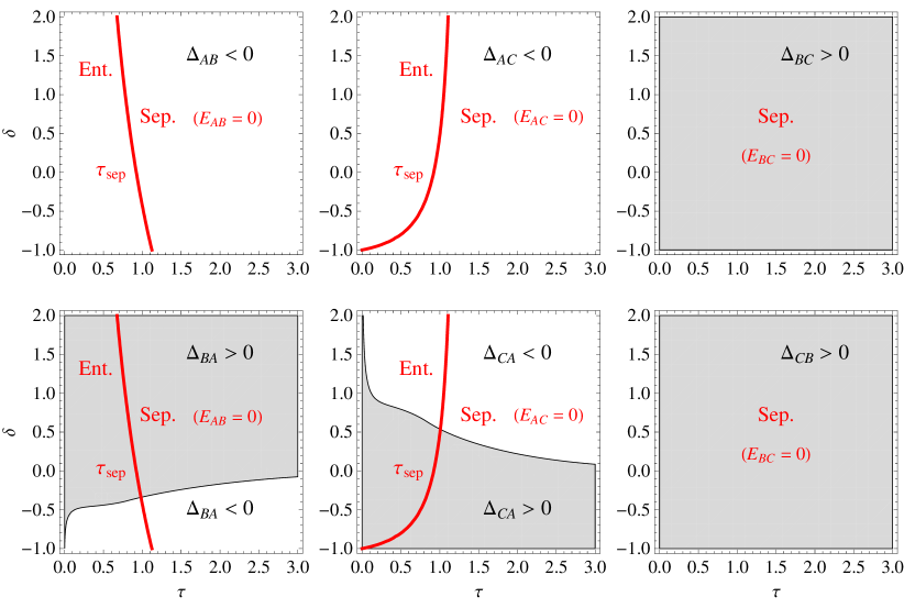
Figure 1: (Color online) Balance of the correlations in the presence of dissipation and thermal noise. Region plots of $\Delta_{hk}$, $h\neq k$ with $h,k=A,B,C$, as functions of $\delta=N_{B}-N_{C}$ of $\tau=\gamma t$. We set $N_{B}=1$ and $N_{\rm th}=0.2$. Gray and white regions refer to the corresponding $\Delta_{hk}>0$ and $\Delta_{hk}<0$, respectively. The red line represents the separability time $\tau_{\rm sep}$: if $\tau\geq\tau_{\rm sep}$ then $\tilde{\lambda}^{(hk)}_{-}\geq\frac{1}{2}$ and the state $\varrho_{hk}(t)$ is no longer entangled (Ent.) and becomes separable (Sep.), i.e., $E_{hk}=0$. See the text for details.

By using the evolved CM (36) and its time-dependent local symplectic invariants, we can calculate the quantities appearing in Eqs. (32). In particular, now one has:

$$f\left(\lambda_{-}^{(hk)}\right)\geq 0\,\quad\hbox{and}\quad f\left(\lambda_{+}^{(hk)}\right)\leq{\mathcal{S}}_{j}$$ (37)

and, in turn, the equalities (34) changes into inequalities. The analytic expressions of the evolved conservation laws may be evaluated analytically, but they are quite clumsy and are not reported here explicitly.

In order to study the evolution of the law (34a) we define the following function:

$$\Delta_{hk}(\tau)=\left[{\mathcal{D}}_{hk}(\tau)+{\mathcal{S}}_{j}(\tau)\right]-\left[{\mathcal{S}}_{h}(\tau)+E_{kj}(\tau)\right]$$ (38)

where all the involved quantities are calculated starting from the results of the previous section but with the evolved state $\varrho_{t}$. As an example, Fig. 1 is a region-plot $\Delta_{hk}(\tau)$ as functions of $\tau$ and $\delta=N_{B}-N_{C}$ for given $N_{B}$ and $N_{\rm th}$: depending on the values of the involved parameters, $\Delta_{hk}(\tau)$ can be positive or negative. In particular, $\Delta_{AB}$ and $\Delta_{AC}$ are always negative, $\Delta_{BA}$ whereas d $\Delta_{CA}$ can change the sign (remarkably, this holds true also for $N_{\rm th}=0$). For the case of symmetric states. i.e., $\delta=0$, one can write the following set of inequalities:

$${\mathcal{D}}_{AB}+{\mathcal{S}}_{C} \leq{\mathcal{S}}_{A}\,, {\mathcal{D}}_{BA}+{\mathcal{S}}_{C} \geq{\mathcal{S}}_{B}+E_{AC}\,,$$ (39a)

$${\mathcal{D}}_{AC}+{\mathcal{S}}_{B} \leq{\mathcal{S}}_{A}\,, {\mathcal{D}}_{CA}+{\mathcal{S}}_{B} \geq{\mathcal{S}}_{C}+E_{AB}\,,$$ (39b)

$${\mathcal{D}}_{BC}+{\mathcal{S}}_{A} \geq{\mathcal{S}}_{B}+E_{CA}\,, {\mathcal{D}}_{CB}+{\mathcal{S}}_{A} \geq{\mathcal{S}}_{C}+E_{BA}\,,$$ (39c)

where we used $E_{BC}=E_{CB}=0$.

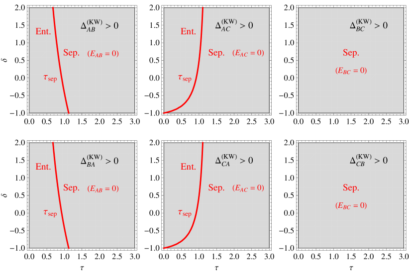
Figure 2: (Color online) Balance of the correlations in the presence of dissipation and thermal noise. Region plots of $\Delta_{hk}^{\rm(KW)}$, $h\neq k$ with $h,k=A,B,C$, as functions of $\delta=N_{B}-N_{C}$ of $\tau=\gamma t$, for the same choice of the other involved parameters as in Fig. 1. Note that one always has $\Delta_{hk}>0$ (gray regions). The red line still represents the separability time $\tau_{\rm sep}$. See the text for details.

Analogously, to address the evolution of the conservation law (34b), we introduce the function:

$$\Delta_{hk}^{\rm(KW)}(\tau)=\left[{\mathcal{D}}_{hk}(\tau)+{\mathcal{S}}_{hk}(\tau)\right]-\left[{\mathcal{S}}_{h}(\tau)+E_{kj}(\tau)\right]\,.$$ (40)

As one can see in Fig. 2, where we plot $\Delta_{hk}^{\rm(KW)}(\tau)$ for the same choice of parameters as in Fig. 1, now one finds the following inequality holding for all the bipartitions, and any value of the interaction time,

$${\mathcal{D}}_{hk}(\tau)+{\mathcal{S}}_{hk}(\tau)\geq{\mathcal{S}}_{h}(\tau)+E_{kj}(\tau)\,,$$ (41)

$h\neq k\neq j$ and $h,k,j=A,B,C$. Ineq. (41) generalizes to CV and Gaussian measures of correlation, the inequality discussed in [31] for the discrete case.

5 Conclusions

In conclusion, we have proved that the balance of correlations originally investigated for three-qubit systems, involving entanglement of formation, quantum discord and single-system entropies is valid also for a feasible class of tripartite Gaussian CV states, upon using Gaussian measures of quantum correlations. Furthermore, in the presence of dissipation and thermal noise, the balance turns into inequalities between the previous quantities, depending on the actual values of the involved parameters. The results are encouraging enough to suggest a direct experimental verification and to foster investigations of correlation balance in more general Gaussian states.

References

References

• [1] B. L. Schumaker, Phys. Rep. 135, 317 (1986).
• [2] A. Ferraro, S. Olivares and M. G. A. Paris, Gaussian States in Quantum Information (Bibliopolis, Napoli 2005)
• [3] G. Adesso, A. Serafini and F. Illuminati, Phys. Rev. Lett. 92, 087901 (2004); 93, 220504 (2004).
• [4] S. L. Braunstein and P. van Loock, Rev. Mod. Phys. 77, 513 (2005).
• [5] A. Ferraro, M. G. A. Paris, Phys. Rev. A 72, 032312 (2005).
• [6] M. M. Wolf, G. Giedke and J. I. Cirac, Phys. Rev. Lett. 96, 080502 (2006).
• [7] C. Weedbrook, S. Pirandola, R. García-Patrón, N. J. Cerf, T. C. Ralph, J. H. Shapiro and S. Lloyd, Rev. Mod. Phys. 84, 621 (2012).
• [8] P. van Loock, and S. Braunstein, Phys. Rev. Lett. 84, 3482 (2000).
• [9] G. Giedke, B. Kraus, M. Lewenstein, and J. I. Cirac, Phys. Rev. A 64, 052303 (2001).
• [10] P. van Loock and A. Furusawa, Phys. Rev. A 67, 052315 (2003).
• [11] P. van Loock, and S. Braunstein, Phys. Rev. Lett. 87, 247901 (2001).
• [12] S. Olivares and M. G. A. Paris, Eur. Phys. J. Special Topics 160, 319 (2008).
• [13] A. Furusawa, J. L. Sørensen, S. L. Braunstein, C. A. Fuchs, H. J. Kimble, and E. S. Polzik, Science 282, 706 (1998).
• [14] J. Zhang, C. Xie, and K. Peng, Phys. Rev. A 66, 032318 (2002).
• [15] J. Jing, J. Zhang, Y. Yan, F. Zhao, C. Xie, K. Peng, Phys. Rev. Lett. 90 167903 (2003).
• [16] T. Aoki, N. Takey, H. Yonezawa, K. Wakui, T. Hiraoka, A. Furusawa, and P. van Loock, Phys. Rev. Lett. 91, 080404 (2003).
• [17] O. Glöckl, S. Lorenz, C. Marquardt, J. Heersink, M. Brownnutt, C. Silberhorn, Q. Pan, P. van Loock, N. Korolkova, and G. Leuchs, Phys. Rev. A 68 012319 (2003).
• [18] A. Allevi, A. Andreoni, M. Bondani, E. Puddu, A. Ferraro, M. G. A. Paris, Opt. Lett. 29, 180 (2004).
• [19] A. Ferraro, M. G. A. Paris, A. Allevi, A. Andreoni, M. Bondani, E. Puddu, J. Opt. Soc. Am. B 21, 1241 (2004).
• [20] P. Giorda and M. G. A. Paris, Phys. Rev. Lett. 105, 020503 (2010).
• [21] G. Adesso and A. Datta, Phys. Rev. Lett 105, 030501 (2010).
• [22] M. Gu, H. M. Chrzanowski, S. M. Assad, T. Symul, K. Modi, T. C. Ralph, V. Vedral, P. K. Lam, arXiv:1203.0011
• [23] R. Blandino, M. G. Genoni, J. Etesse, M. Barbieri, M. G. A. Paris, P. Grangier, R. Tualle-Brouri, arXiv:1203.1127
• [24] L. S. Madsen, A. Berni, M. Lassen, U. L. Andersen, arXiv:1204.2738
• [25] M. Koashi, A. Winter, Phys. Rev. A 69, 022309 (2004).
• [26] A. Kay, D. Kaszlikowski, and R. Ramanathan, Phys. Rev. Lett. 103, 050501 (2009).
• [27] M. Pawlowski and C. Brukner, Phys. Rev. Lett. 102, 030403 (2009).
• [28] M. Seevinck, Quant. Inf. Proc. 9, 273 (2010).
• [29] R. Prabhu, A. K. Pati, A. Sen(De), and U. Sen, Phys. Rev. A 85, 040102(R) (2012).
• [30] G. L. Giorgi, Phys. Rev. A 84, 054301 (2011).
• [31] F. F. Fanchini, M. F. Cornelio, M. C. de Oliveira, and A. O. Caldeira, Phys. Rev. A 84, 012313 (2011).
• [32] X-J. Ren, H. Fan, arXiv:1111.5163, (2011).
• [33] K. Modi, A. Brodutch, H. Cable, T. Paterek, V. Vedral, arXiv:1112.6238.
• [34] G. Adesso, D. Girolami, A. Serafini, arXiv:1203.5116, (2012).
• [35] A. Streltsov, H. Kampermann, D. Bruss, Phys. Rev. Lett. 106, 160401 (2011).
• [36] F. Ciccarello, V. Giovannetti Phys. Rev. A 85, 010102 (2012).
• [37] S. Campbell, T. J. G. Apollaro, C. Di Franco, L. Banchi, A. Cuccoli, R. Vaia, F. Plastina, and M. Paternostro Phys. Rev. A 84, 052316 (2011).
• [38] M. Gessner, E-M. Laine, H-P. Breuer, J. Piilo, Phys. Rev. A 85, 052122 (2012).
• [39] T. K. Chuan, J. Maillard, K. Modi, T. Paterek, M. Paternostro, M. Piani, arXiv:1203.1268.
• [40] A. Streltsov, H. Kampermann, D. Bruss, Phys. Rev. Lett. 108, 250501 (2012).
• [41] P. Giorda, M. Allegra, M. G. A. Paris, arXiv:1206.1807, (2012).
• [42] A. Ferraro, M. G. A. Paris, Phys. Rev. Lett 108, 260403 (2012).
• [43] R. A. Andrews, H. Rabin, and C. L. Tang, Phys. Rev. Lett. 25, 605 (1970).
• [44] M. E. Smithers, E. Y. C. Lu, Phys. Rev. A 10, 1874 (1974).
• [45] M. G. A. Paris, M. Cola, N. Piovella and R. Bonifacio, Opt. Comm. 227, 349 (2003).
• [46] M. M. Cola, M. G. A. Paris and N. Piovella, Phys. Rev. A 70, 043809 (2004)
• [47] S. Olivares, Eur. Phys. J. Special Topics 203, 3 (2012)
• [48] G. Giedke, M. M. Wolf, O. Krüger, R. F. Werner, and J. I. Cirac, Phys. Rev. Lett. 91, 107901 (2003).
• [49] P. Marian and T. A. Marian, Phys. Rev. Lett. 101, 220403 (2008).