Computing n-Gram Statistics in MapReduce

Abstract

Statistics about $n$-grams (i.e., sequences of contiguous words or other tokens in text documents or other string data) are an important building block in information retrieval and natural language processing. In this work, we study how $n$-gram statistics, optionally restricted by a maximum $n$-gram length and minimum collection frequency, can be computed efficiently harnessing MapReduce for distributed data processing. We describe different algorithms, ranging from an extension of word counting, via methods based on the Apriori principle, to a novel method Suffix-$\sigma$ that relies on sorting and aggregating suffixes. We examine possible extensions of our method to support the notions of maximality/closedness and to perform aggregations beyond occurrence counting. Assuming Hadoop as a concrete MapReduce implementation, we provide insights on an efficient implementation of the methods. Extensive experiments on The New York Times Annotated Corpus and ClueWeb09 expose the relative benefits and trade-offs of the methods.

I Introduction

Applications in various fields including information retrieval [12, 46] and natural language processing [13, 18, 39] rely on statistics about $n$-grams (i.e., sequences of contiguous words in text documents or other string data) as an important building block. Google and Microsoft have made available $n$-gram statistics computed on parts of the Web. While certainly a valuable resource, one limitation of these datasets is that they only consider $n$-grams consisting of up to five words. With this limitation, there is no way to capture idioms, quotations, poetry, lyrics, and other types of named entities (e.g., products, books, songs, or movies) that typically consist of more than five words and are crucial to applications including plagiarism detection, opinion mining, and social media analytics.

MapReduce has gained popularity in recent years both as a programming model and in its open-source implementation Hadoop. It provides a platform for distributed data processing, for instance, on web-scale document collections. MapReduce imposes a rigid programming model, but treats its users with features such as handling of node failures and an automatic distribution of the computation. To make most effective use of it, problems need to be cast into its programming model, taking into account its particularities.

In this work, we address the problem of efficiently computing $n$-gram statistics on MapReduce platforms. We allow for a restriction of the $n$-gram statistics to be computed by a maximum length $\sigma$ and a minimum collection frequency $\tau$. Only $n$-grams consisting of up to $\sigma$ words and occurring at least $\tau$ times in the document collection are thus considered.

While this can be seen as a special case of frequent sequence mining, our experiments on two real-world datasets show that MapReduce adaptations of Apriori-based methods [38, 44] do not perform well – in particular when long and/or less frequent $n$-grams are of interest. In this light, we develop our novel method Suffix-$\sigma$ that is based on ideas from string processing. Our method makes thoughtful use of MapReduce’s grouping and sorting functionality. It keeps the number of records that have to be sorted by MapReduce low and exploits their order to achieve a compact main-memory footprint, when determining collection frequencies of all $n$-grams considered.

We also describe possible extensions of our method. This includes the notions of maximality/closedness, known from frequent sequence mining, that can drastically reduce the amount of $n$-gram statistics computed. In addition, we investigate to what extent our method can support aggregations beyond occurrence counting, using $n$-gram time series, recently made popular by Michel et al. [32], as an example.

Contributions made in this work include:

• a novel method Suffix-$\sigma$ to compute $n$-gram statistics that has been specifically designed for MapReduce;

• a detailed account on efficient implementation and possible extensions of Suffix-$\sigma$ (e.g., to consider maximal/closed $n$-grams or support other aggregations);

• a comprehensive experimental evaluation on The New York Times Annotated Corpus (1.8 million news articles from 1987–2007) and ClueWeb09-B (50 million web pages crawled in 2009), as two large-scale real-world datasets, comparing our method against state-of-the-art competitors and investigating their trade-offs.

Suffix-$\sigma$ outperforms its best competitor in our experiments by up to a factor 12x when long and/or less frequent $n$-grams are of interest. Otherwise, it performs at least on par with the best competitor.

Organization. Section II introduces our model. Section III details on methods to compute $n$-gram statistics based on prior ideas. Section IV introduces our method Suffix-$\sigma$. Aspects of efficient implementation are addressed in Section V. Possible extensions of Suffix-$\sigma$ are sketched in Section VI. Our experiments are the subject of Section VII. In Section VIII, we put our work into context, before concluding in Section IX.

II Preliminaries

We now introduce our model, establish our notation, and provide some technical background on MapReduce.

II-A Data Model

Our methods operate on sequences of terms (i.e., words or other textual tokens) drawn from a vocabulary $\mathcal{V}$. We let $\mathcal{S}$ denote the universe of all sequences over $\mathcal{V}$. Given a sequence $\mathbf{s}=\langle\,s_{0},\ldots,s_{n-1}\,\rangle$ with $s_{i}\in\mathcal{V}$, we refer to its length as $|\mathbf{s}|$, write $\mathbf{s}[i..j]$ for the subsequence $\langle\,s_{i},\ldots,s_{j}\,\rangle$, and let $\mathbf{s}[i]$ refer to the element $s_{i}$. For two sequences $\mathbf{r}$ and $\mathbf{s}$, we let $\mathbf{r}\|\mathbf{s}$ denote their concatenation. We say that

• $\mathbf{r}$ is a prefix of $\mathbf{s}$ ($\mathbf{r}\triangleright\mathbf{s}$) iff

  $$\forall{\,0\leq i<|\mathbf{r}|}\>:\>\mathbf{r}[i]=\mathbf{s}[i]$$

• $\mathbf{r}$ is a suffix of $\mathbf{s}$ ($\mathbf{r}\triangleleft\mathbf{s}$) iff

  $$\forall{\,0\leq i<|\mathbf{r}|}\>:\>\mathbf{r}[i]=\mathbf{s}[|\mathbf{s}|-|\mathbf{r}|+i]$$

• $\mathbf{r}$ is a subsequence of $\mathbf{s}$ ($\mathbf{r}\diamond\mathbf{s}$) iff

  $$\exists{\,0\leq j<|\mathbf{s}|}\>:\>\forall{\,0\leq i<|\mathbf{r}|}\>:\>\mathbf{r}[i]=\mathbf{s}[i+j]$$

and capture how often $\mathbf{r}$ occurs in $\mathbf{s}$ as

$$f(\mathbf{r},\mathbf{s})=\left|\left\{\,0\leq j<|\mathbf{s}|\>\>|\>\>\forall{\,0\leq i<|\mathbf{r}|}\>:\>\mathbf{r}[i]=\mathbf{s}[i+j]\,\right\}\right|\;.$$

To avoid confusion, we use the following convention: When referring to sequences of terms having a specific length $k$, we will use the notion $k$-gram or indicate the considered length by alluding to, for instance, $5$-grams. The notion $n$-gram, as found in the title, will be used when referring to variable-length sequences of terms.

As an input, all methods considered in this work receive a document collection $\mathcal{D}$ consisting of sequences of terms as documents. Our focus is on determining how often $n$-grams occur in the document collection. Formally, the collection frequency of an $n$-gram $\mathbf{s}$ is defined as as $cf(\mathbf{s})=\sum_{\mathbf{d}\in\mathcal{D}}f(\mathbf{s},\mathbf{d})\;.$ Alternatively, one could consider the document frequency of $n$-grams as the total number of documents that contain a specific $n$-gram. While this corresponds to the notion of support typically used in frequent sequence mining, it is less common for natural language applications. However, all methods presented below can easily be modified to produce document frequencies instead.

II-B MapReduce

MapReduce, as described by Dean and Ghemawat [17], is a programming model and an associated runtime system at Google. While originally proprietary, the MapReduce programming model has been widely adopted in practice and several implementations exist. In this work, we rely on Hadoop [1] as a popular open-source MapReduce platform. The objective of MapReduce is to facilitate distributed data processing on large-scale clusters of commodity computers. MapReduce enforces a functional style of programming and lets users express their tasks as two functions

map()	:	(k1,v1) -> list<(k2,v2)>
reduce()	:	(k2, list<v2>) -> list<(k3,v3)>

that consume and emit key-value pairs. Between the map- and reduce-phase, the system sorts and groups the key-value pairs emitted by the map-function. The partitioning of key-value pairs (i.e., how they are assigned to cluster nodes) and their sort order (i.e., in which order they are seen by the reduce-function on each cluster node) can be customized, if needed for the task at hand. For detailed introductions to working with MapReduce and Hadoop, we refer to Lin and Dyer [29] as well as White [41].

III Methods based on prior ideas

With our notation established, we next describe three methods based on prior ideas to compute $n$-gram statistics in MapReduce. Before delving into their details, let us state the problem that we address in more formal terms:

Given a document collection $\mathcal{D}$, a minimum collection frequency $\tau$, a maximum length $\sigma$, our objective is to identify all $n$-grams $\mathbf{s}$ with their collection frequency $cf(\mathbf{s})$, for which $cf(\mathbf{s})\geq\tau$ and $|\mathbf{s}|\leq\sigma$ hold.

We thus assume that $n$-grams are only of interest to the task at hand, if they occur at least $\tau$ times in the document collection, coined frequent in the following, and consist of at most $\sigma$ terms. Consider, as an example task, the construction of $n$-gram language models [46], for which one would only look at $n$-grams up to a specific length and/or resort to back-off models [24] to obtain more robust estimates for $n$-grams that occur less than specific number of times.

The problem statement above can be seen as a special case of frequent sequence mining that considers only contiguous sequences of single-element itemsets. We believe this to be an important special case that warrants individual attention and allows for an efficient solution in MapReduce, as we show in this work. A more elaborate comparison to existing research on frequent sequence mining is part of Section VIII.

To ease our explanations below, we use the following running example, considering a collection of three documents:

$\mathbf{d}_{1}$	=	$\langle\,$a x b x x$\,\rangle$
$\mathbf{d}_{2}$	=	$\langle\,$b a x b x$\,\rangle$
$\mathbf{d}_{3}$	=	$\langle\,$x b a x b$\,\rangle$

With parameters $\tau=3$ and $\sigma=3$, we expect as output

$\langle\,$a$\,\rangle$	:	$3$	$\langle\,$b$\,\rangle$	:	$5$	$\langle\,$x$\,\rangle$	:	$7$
$\langle\,$a x$\,\rangle$	:	$3$	$\langle\,$x b$\,\rangle$	:	$4$
$\langle\,$a x b$\,\rangle$	:	$3$

from any method, when applied to this document collection.

III-A Naïve Counting

One of the example applications of MapReduce, given by Dean and Ghemawat [17] and also used in many tutorials, is word counting, i.e., determining the collection frequency of every word in the document collection. It is straightforward to adapt word counting to consider variable-length $n$-grams instead of only unigrams and discard those that occur less than $\tau$ times. Pseudo code of this method, which we coin Naïve, is given in Algorithm 1.

// Mapper

0 map(long $did$, seq $\mathbf{d}$) begin

      

      2for $b=0$ to $|\mathbf{d}|-1$ do

            3 for $e=b$ to $min(b+\sigma-1,|\mathbf{d}|-1)$ do

                  4 emit(seq $\mathbf{d}[b..e]$, long $did$)

            

      

// Reducer

0 reduce(seq $\mathbf{s}$, list<long> $l$) begin

      

      2if $|l|\geq\tau$ then

            

            4emit(seq $\mathbf{s}$, int $|l|$)

      

Algorithm 1 Naïve

In the map-function, the method emits all $n$-grams of length up to $\sigma$ for a document together with the document identifier. If an $n$-gram occurs more than once, it is emitted multiple times. In the reduce-phase, the collection frequency of every $n$-gram is determined and, if it exceeds $\tau$, emitted together with the $n$-gram itself.

Interestingly, apart from minor optimizations, this is the method that Brants et al. [13] used for training large-scale language models at Google, considering $n$-grams up to length five. In practice, several tweaks can be applied to improve this simple method including local pre-aggregation in the map-phase (e.g., using a combiner in Hadoop). Implementation details of this kind are covered in more detail in Section V. The potentially vast number of emitted key-value pairs that needs to be transferred and sorted, though, remains a shortcoming.

In the worst case, when $\sigma\geq|\mathbf{d}|$, Naïve emits $\mathcal{O}(|\mathbf{d}|^{2})$ key-value pairs for a document $\mathbf{d}$, each consuming $\mathcal{O}(|\mathbf{d}|)$ bytes, so that the method transfers $\mathcal{O}(|\mathbf{d}|^{3})$ bytes between the map- and reduce-phase. Complementary to that, we can determine the number of key-value pairs emitted based on the $n$-gram statistics. Naïve emits a total of $\sum_{\mathbf{s}\in\mathcal{S}:|\mathbf{s}|\leq\sigma}cf(\mathbf{s})$ key-value pairs, each of which consumes $\mathcal{O}(|\mathbf{s}|)$ bytes.

III-B Apriori-Based Methods

How can one do better than the naïve method just outlined? One idea is to exploit the Apriori principle, as described by Agrawal et al. [9] in their seminal paper on identifying frequent itemsets and follow-up work on frequent pattern mining [10, 37, 38, 44]. Cast into our setting, the Apriori principle states that

$$\mathbf{r}\diamond\mathbf{s}\quad\Rightarrow\quad cf(\mathbf{r})\geq cf(\mathbf{s})$$

holds for any two sequences $\mathbf{r}$ and $\mathbf{s}$, i.e., the collection frequency of a sequence $\mathbf{r}$ is an upper bound for the collection frequency of any supersequence $\mathbf{s}$. In what follows, we describe two methods that make use of the Apriori principle to compute $n$-gram statistics in MapReduce.

Apriori-Scan

The first Apriori-based method Apriori-Scan, like the original Apriori algorithm [9] and GSP [38], performs multiple scans over the input data. During the $k$-th scan the method determines $k$-grams that occur at least $\tau$ times in the document collection. To this end, it exploits the output from the previous scan via the Apriori principle to prune the considered $k$-grams. In the $k$-th scan, only those $k$-grams are considered whose two constituent $(k-1)$-grams are known to be frequent. Unlike GSP, that first generates all potentially frequent sequences as candidates, Apriori-Scan considers only sequences that actually occur in the document collection. The method terminates after $\sigma$ scans or when a scan does not produce any output.

Algorithm 2 shows how the method can be implemented in MapReduce. The outer repeat-loop controls the execution of multiple MapReduce jobs, each of which performs one distributed parallel scan over the input data. In the $k$-th iteration, and thus the $k$-th scan of the input data, the method considers all $k$-grams from an input document in the map-function, but discards those that have a constituent $(k-1)$-gram that is known to be infrequent. This pruning is done, leveraging the output from the previous iteration that is kept in a dictionary. In the reduce-function, analogous to Naïve, collection frequencies of $k$-grams are determined and output if above the minimum collection frequency $\tau$. After $\sigma$ iterations or once an iteration does not produce any output, the method terminates, which is safe since the Apriori principle guarantees that no longer $n$-gram can occur $\tau$ or more times in the document collection.

int $k=1$

repeat

      

      hashset<int[]> $dict=$ load(output-$(k-1)$)

      // Mapper

      

      1map(long $did$, seq $\mathbf{d}$) begin

            

            3for $b=0$ to $|\mathbf{d}|-k$ do

                  

                  5if $k=1$ $\vee$

                  6 $($contains(dict, $\mathbf{d}[b..(b+k-2)]$) $\wedge$

                  7  contains(dict, $\mathbf{d}[(b+1)..(b+k-1)]$$)$) then

                        8 emit(seq $\mathbf{d}[b..(b+k-1)]$, long $did$)

                  

            

      

      // Reducer

      

      1reduce(seq $\mathbf{s}$, list<long> $l$) begin

            

            3if $|l|\geq\tau$ then

                  

                  5emit(seq $\mathbf{s}$, int $|l|$)

            

      

      

      $k$ += $1$

until isEmpty(output-$(k-1)$) $\vee$ $k=\sigma+1$;

Algorithm 2 Apriori-Scan

When applied to our running example, in its third scan of the input data, Apriori-Scan emits in the map-phase for every document $\mathbf{d}_{i}$ only the key-value pair $($$\langle\,$a x b$\,\rangle$$,\mathbf{d}_{i})$, but discards other trigrams (e.g., $\langle\,$b x x$\,\rangle$) that contain an infrequent bigram (e.g., $\langle\,$x x$\,\rangle$).

When implemented in MapReduce, every iteration corresponds to a separate job that needs to be run and comes with its administrative fix cost (e.g., for launching and finalizing the job). Another challenge in Apriori-Scan is the implementation of the dictionary that makes the output from the previous iteration available and accessible to cluster nodes. This dictionary can either be implemented locally, so that every cluster node receives a replica of the previous iteration’s output (e.g., implemented using the distributed cache in Hadoop), or, by loading the output from the previous iteration into a shared dictionary (e.g., implemented using a distributed key-value store) that can then be accessed remotely by cluster nodes. Either way, to make lookups in the dictionary efficient, significant main memory at cluster nodes is required.

An apparent shortcoming of Apriori-Scan is that it has to scan the entire input data in every iteration. Thus, although typically only few frequent $n$-grams are found in later iterations, the cost of an iteration depends on the size of the input data. The number of iterations needed, on the other hand, is determined by the parameter $\sigma$ or the length of the longest frequent $n$-gram.

In the worst case, when $\sigma\geq|\mathbf{d}|$ and $cf(\mathbf{d})\geq\tau$, Apriori-Scan emits $\mathcal{O}(|\mathbf{d}|^{2})$ key-value pairs per document $\mathbf{d}$, each consuming $\mathcal{O}(|\mathbf{d}|)$ bytes, so that the method transfers $\mathcal{O}(|\mathbf{d}|^{3})$ bytes between the map- and reduce-phase. Again, we provide a complementary analysis based on the actual $n$-gram statistics. To this end, let

$$\mathcal{S}_{NP}=\left\{\mathbf{s}\in\mathcal{S}\>|\>\forall{\,\mathbf{r}\in\mathcal{S}}\>:\>(\mathbf{r}\neq\mathbf{s}\>\wedge\>\mathbf{r}\diamond\mathbf{s})\Rightarrow cf(\mathbf{r})\geq\tau\right\}$$

denote the set of sequences that cannot be pruned based on the Apriori principle, i.e., whose true subsequences all occur at least $\tau$ times in the document collection. Apriori-Scan emits a total of $\sum_{\mathbf{s}\in\mathcal{S}_{NP}:|\mathbf{s}|\leq\sigma}cf(\mathbf{s})$ key-value pairs, each of which amounts to $\mathcal{O}(|\mathbf{s}|)$ bytes. Obviously, $\mathcal{S}_{NP}\subseteq\mathcal{S}$ holds, so that Apriori-Scan emits at most as many key-value pairs as Naïve. Its concrete gains, though, depend on the value of $\tau$ and characteristics of the document collection.

Apriori-Index

The second Apriori-based method Apriori-Index does not repeatedly scan the input data but incrementally builds an inverted index of frequent $n$-grams from the input data as a more compact representation. Operating on an index structure as opposed to the original data and considering $n$-grams of increasing length, it resembles SPADE [44] when breadth-first traversing the sequence lattice.

int $k$ $=$ $1$

repeat

      

      if $k\leq\mathtt{K}$ then

            

            // Mapper #1

            

            1map(long $did$, seq $\mathbf{d}$) begin

                  

                  3hashmap<seq, int[]> pos $=\emptyset$

                  4for $b=0$ to $|\mathbf{d}|-1$ do

                        

                        6add(get(pos, $\mathbf{d}[b..(b+k-1)]$), $b$)

                  

                  8for seq $\mathbf{s}$ : keys(pos) do

                        9 emit(seq $\mathbf{s}$, posting $($$did$, get(pos,$\mathbf{s}$)$)$)

                  

            

            // Reducer #1

            

            1reduce(seq $\mathbf{s}$, list<posting> $l$) begin

                  

                  3if cf($l$) $\geq\tau$ then

                        

                        5emit(seq $\mathbf{s}$, list<posting> $l$)

                  

            

      else

            

            

            // Mapper #2

            

            1map(seq $\mathbf{s}$, list<posting> $l$) begin

                  

                  3emit(seq $\mathbf{s}[0..|\mathbf{s}|-2]$,

                  4    $($r-seq, list<posting>$)$ $(\mathbf{s},l)$)

                  5emit(seq $\mathbf{s}[1..|\mathbf{s}|-1]$,

                  6    $($l-seq, list<posting>$)$ $(\mathbf{s},l)$)

            

            // Reducer #2

            

            1reduce(seq $\mathbf{s}$, list<$($seq, list<posting>$)$> $l$) begin

                  

                  3for $($l-seq, list<posting>$)$ $(\mathbf{m},l_{m})$ : $l$ do

                        

                        5for $($r-seq, list<posting>$)$ $(\mathbf{n},l_{n})$ : $l$ do

                              

                              7list<posting> $l_{j}$ = join($l_{m}$, $l_{n}$)

                              8if cf($l_{j}$) $\geq\tau$ then

                                    

                                    10seq $\mathbf{j}$ $=\mathbf{m}\,\|\,\langle\,\mathbf{n}[|\mathbf{n}|-1]\,\rangle$

                                    11emit(seq $\mathbf{j}$, list<posting> $l_{j}$)

                              

                        

                  

            

      

      $k$ += $1$

until isEmpty(output-$(k-1)$) $\vee$ $k=$ $min(\sigma,\mathtt{K})$;

Algorithm 3 Apriori-Index

Pseudo code of Apriori-Index is given in Algorithm 3. In its first phase, the method constructs an inverted index with positional information for all frequent $n$-grams up to length $\mathtt{K}$ (cf. Mapper #1 and Reducer #1 in the pseudo code). In its second phase, to identify frequent $n$-grams beyond that length, Apriori-Index harnesses the output from the previous iteration. Thus, to determine a frequent $k$-gram (e.g., $\langle\,$b a x$\,\rangle$), the method joins the posting lists of its constituent $(k-1)$-grams (i.e., $\langle\,$b a$\,\rangle$ and $\langle\,$a x$\,\rangle$). In MapReduce, this can be accomplished as follows (cf. Mapper #2 and Reducer #2 in the pseudo code): The map-function emits for every frequent $(k-1)$-gram two key-value pairs. The frequent $(k-1)$-gram itself along with its posting list serves in both as a value. As keys the prefix and suffix of length $(k-2)$ are used. In the pseudo code, the method keeps track of whether the key is a prefix or suffix of the sequence in the value by using the r-seq and l-seq subtypes. The reduce-function identifies for a specific key all compatible sequences from the values, joins their posting lists, and emits the resulting $k$-gram along with its posting list if its collection frequency is at least $\tau$. Two sequences are compatible and must be joined, if one has the current key as a prefix, and the other has it as a suffix. In its nested for-loops, the method considers all compatible combinations of sequences. This second phase of Apriori-Index can be seen as a distributed candidate generation and pruning step.

Applied to our running example and assuming $K=2$, the method only sees one pair of compatible sequences with their posting lists for the key $\langle\,$x$\,\rangle$ in its third iteration, namely:

$\langle\,$a x$\,\rangle$	:	$\langle\,\mathbf{d}_{1}:[0],\>\>\mathbf{d}_{2}:[1],\>\>\mathbf{d}_{3}:[2]\,\rangle$
$\langle\,$x b$\,\rangle$	:	$\langle\,\mathbf{d}_{1}:[1],\>\>\mathbf{d}_{2}:[2],\>\>\mathbf{d}_{3}:[0,3]\,\rangle\;.$

By joining those, Apriori-Index obtains the only frequent $3$-gram with its posting list

$\langle\,$a x b$\,\rangle$

:

$\langle\,\mathbf{d}_{1}:[0],\>\>\mathbf{d}_{2}:[1],\>\>\mathbf{d}_{3}:[2]\,\rangle\;.$

For all $k<\mathtt{K}$, it would be enough to determine only collection frequencies, as opposed to, positional information of $n$-grams. While a straightforward optimization in practice, we opted for simpler pseudo code. When implemented as described in Algorithm 3, the method produces an inverted index with positional information that can be used to quickly determine the locations of a specific frequent $n$-gram.

One challenge when implementing Apriori-Index is that the number and size of posting-list values seen for a specific key can become large in practice. Moreover, to join compatible sequences, these posting lists have to be buffered, and a scalable implementation must deal with the case when this is not possible in the available main memory. This can, for instance, be accomplished by storing posting lists temporarily in a disk-resident key-value store.

The number of iterations needed by Apriori-Index is determined by the parameter $\sigma$ or the length of the longest frequent $n$-gram. Since every iteration, as for Apriori-Scan, corresponds to a separate MapReduce job, a non-negligible administrative fix cost is incurred.

In the worst case, when $\sigma\geq|\mathbf{d}|$ and $cf(\mathbf{d})\geq\tau$, Apriori-Index emits $\mathcal{O}(|\mathbf{d}|^{2})$ key-value pairs per document $\mathbf{d}$, each consuming $\mathcal{O}(|\mathbf{d}|)$ bytes, so that $\mathcal{O}(|\mathbf{d}|^{3})$ bytes are transferred the map- and reduce-phase. We assume $K<\sigma$ for the complementary analysis. In its first $K$ iterations, Apriori-Index emits $\sum_{\mathbf{s}\in\mathcal{S}:|\mathbf{s}|\leq K}df(\mathbf{s})$ key-value pairs, where $df(\mathbf{s})\leq cf(\mathbf{s})$ refers to the document frequency of the $n$-gram $\mathbf{s}$, as mentioned in Section II. Each key-value pair consumes $\mathcal{O}(cf(\mathbf{s}))$ bytes. To analyze the following iterations, let

$$\mathcal{S}_{F}=\left\{\mathbf{s}\in\mathcal{S}\>|\>cf(\mathbf{s})\geq\tau\right\}$$

denote the set of frequent $n$-grams that occur at least $\tau$ times. Apriori-Index emits a total of

$$2\cdot|\{\mathbf{s}\in\mathcal{S}_{F}\>|\>K\leq|\mathbf{s}|<\sigma\}|$$

key-value pairs, each of which consumes $\mathcal{O}(cf(\mathbf{s}))$ bytes. Like for Apriori-Scan, the concrete gains depend on the value of $\tau$ and characteristics of the document collection.

IV Suffix sorting & aggregation

As already argued, the methods presented so far suffer from either excessive amounts of data that need to be transferred and sorted, requiring possibly many MapReduce jobs, or a high demand for main memory at cluster nodes. Our novel method Suffix-$\sigma$ avoids these deficiencies: It requires a single MapReduce job, transfers only a modest amount of data, and requires little main memory at cluster nodes.

Consider again what the map-function in the Naïve approach emits for document $\mathbf{d}_{3}$ from our running example. Emitting key-value pairs for all of the $n$-grams $\langle\,$b a x$\,\rangle$, $\langle\,$b a$\,\rangle$, and $\langle\,$b$\,\rangle$ is clearly wasteful. The key observation here is that the latter two are subsumed by the first one and can be obtained as its prefixes. Suffix arrays [31] and other string processing techniques exploit this very idea.

Based on this observation, it is safe to emit key-value pairs only for a subset of the $n$-grams contained in a document. More precisely, it is enough to emit at every position in the document a single key-value pair with the suffix starting at that position as a key. These suffixes can further be truncated to length $\sigma$ – hence the name of our method.

// Mapper

1map(long $did$, seq $\mathbf{d}$) begin

      2 for $b=0$ to $|\mathbf{d}|-1$ do

            3 emit(seq $\mathbf{d}[b..min(b+\sigma-1,|\mathbf{d}|-1)]$, long $did$)

      

// Reducer

stack<int> $terms=\emptyset$

stack<int> $counts=\emptyset$

1reduce(seq $\mathbf{s}$, list<long> $l$) begin

      

      3while lcp(s,seq($terms$)) $<$ len($terms$) do

            

            5if peek($counts$) $\geq\tau$  then

                  

                  7emit(seq seq($terms$), int peek($counts$))

            

            9pop($terms$)

            10push($counts$, pop($counts$) + pop($counts$))

      

      12if len($terms$) $=|\mathbf{s}|$ then

            1313push($counts$, pop($counts$) + $|l|$)

      else

            15 for $i=$ lcp(s, seq($terms$)) to $|\mathbf{s}|-1$ do

                  16 push($terms$, $\mathbf{s}[i]$)

                  17push($counts$, $(i==|\mathbf{s}|-1$ ? $|l|$ : $0)$)

            

      

1cleanup() begin

      2 reduce(seq $\emptyset$, list<long> $\emptyset$)

// Partitioner

1partition(seq $\mathbf{s}$) begin

      

      3return hashcode($\mathbf{s}[0]$) mod $R$

// Comparator

1compare(seq $r$, seq $s$) begin

      2 for $b=0$ to $min(|\mathbf{r}|,|\mathbf{s}|)-1$ do

            3 if $\mathbf{r}[b]<\mathbf{s}[b]$ then

                  4 return $+1$

            5 else if $\mathbf{r}[b]>\mathbf{s}[b]$ then

                  6 return $-1$

            

      8return $|\mathbf{s}|-|\mathbf{r}|$

Algorithm 4 Suffix-$\sigma$

To determine the collection frequency of a specific $n$-gram $\mathbf{r}$, we have to determine how many of the suffixes emitted in the map-phase are prefixed by $\mathbf{r}$. To do so correctly using only a single MapReduce job, we must ensure that all relevant suffixes are seen by the same reducer. This can be accomplished by partitioning suffixes based on their first term only, as opposed to, all terms therein. It is thus guaranteed that a single reducer receives all suffixes that begin with the same term. This reducer is then responsible for determining the collection frequencies of all $n$-grams starting with that term. One way to accomplish this would be to enumerate all prefixes of a received suffix and aggregate their collection frequencies in main memory (e.g., using a hashmap or a prefix tree). Since it is unknown whether an $n$-gram is represented by other yet unseen suffixes from the input, it cannot be emitted early along with its collection frequency. Bookkeeping is thus needed for many $n$-grams and requires significant main memory.

How can we reduce the main-memory footprint and emit $n$-grams with their collection frequency early on? The key idea is to exploit that the order in which key-value pairs are sorted and received by reducers can be influenced. Suffix-$\sigma$ sorts key-value pairs in reverse lexicographic order of their suffix key, formally defined as follows for sequences $\mathbf{r}$ and $\mathbf{s}$:

$$\mathbf{r}<\mathbf{s}\Leftrightarrow(|\mathbf{r}|>|\mathbf{s}|\>\wedge\>\mathbf{s}\triangleright\mathbf{r})\>\vee\>\hskip 125.19194pt$$

$$\exists{\,0\!\leq\!i<min(|\mathbf{r}|,|\mathbf{s}|)}\!:\!\mathbf{r}[i]>\mathbf{s}[i]\wedge\forall{\,0\!\leq\!j<i}:\mathbf{r}[j]=\mathbf{s}[j]\;.$$

To see why this is useful, recall that each suffix from the input represents all $n$-grams that can be obtained as its prefixes. Let $\mathbf{s}$ denote the current suffix from the input. The reverse lexicographic order guarantees that we can safely emit any $n$-gram $\mathbf{r}$ such that $\mathbf{r}<\mathbf{s}$, since no yet unseen suffix from the input can represent $\mathbf{r}$. Conversely, at this point, the only $n$-grams for which we have to do bookkeeping, since they are represented both by the current suffix $\mathbf{s}$ and potentially by yet unseen suffixes, are the prefixes of $\mathbf{s}$. We illustrate this observation with our running example. The reducer responsible for suffixes starting with b receives:

$\langle\,$b x x$\,\rangle$	:	$\langle\,\mathbf{d}_{1}\,\rangle$
$\langle\,$b x$\,\rangle$	:	$\langle\,\mathbf{d}_{2}\,\rangle$
$\langle\,$b a x$\,\rangle$	:	$\langle\,\mathbf{d}_{2},\>\>\mathbf{d}_{3}\,\rangle$
$\langle\,$b$\,\rangle$	:	$\langle\,\mathbf{d}_{3}\,\rangle\;.$

When seeing the third suffix $\langle\,$b a x$\,\rangle$, we can immediately finalize the collection frequency of the $n$-gram $\langle\,$b x$\,\rangle$ and emit it, since no yet unseen suffix can have it as a prefix. On the contrary, the $n$-grams $\langle\,$b$\,\rangle$ and $\langle\,$b a$\,\rangle$ cannot be emitted, since yet unseen suffixes from the input may have them as a prefix.

Building on this observation, we can do efficient bookkeeping for prefixes of the current suffix $\mathbf{s}$ only and lazily aggregate their collection frequencies using two stacks. On the first stack $terms$, we keep the terms constituting $\mathbf{s}$. The second stack $counts$ keeps one counter per prefix of $\mathbf{s}$. Between invocations of the reduce-function, we maintain two invariants. First, the two stacks have the same size $m$. Second, $\sum_{j=i}^{m-1}counts[j]$ reflects how often the $n$-gram $\langle\,terms[0],\,\ldots,\,terms[i]\,\rangle$ has been seen so far in the input. To maintain these invariants, when processing a suffix $\mathbf{s}$ from the input, we first synchronously pop elements from both stacks until the contents of $terms$ form a prefix of $\mathbf{s}$. Before each pop operation, we emit the contents of $terms$ and the top element of $counts$, if the latter is above our minimum collection frequency $\tau$. When popping an element from $counts$, its value is added to the new top element. Following that, we update $terms$, so that its contents equal the suffix $\mathbf{s}$. For all but the last term added, a zero is put on $counts$. For the last term, we put the frequency of $\mathbf{s}$, reflected by the length of its associated document-identifier list value, on $counts$. Figure 1 illustrates how the states of the two stacks evolve, as the above example input is processed.

x 1		x 2
x 0	x 2	a 0
b 0	b 0	b 2	b 4	_ _

Figure 1: Suffix-$\sigma$’s bookkeeping illustrated

Pseudo code of Suffix-$\sigma$ is given in Algorithm 4. The map-function emits for every document all its suffixes truncated to length $\sigma$ if possible. The reduce-function reads suffixes in reverse lexicographic order and performs the bookkeeping using two separate stacks for $n$-grams (terms) and their collection frequencies (counts), as described above. The function seq() returns the $n$-gram corresponding to the entire terms stack. The function lcp() returns the length of the longest common prefix that two $n$-grams share. In addition, Algorithm 4 contains a partition-function ensuring that suffixes are assigned to one of $R$ reducers solely based on their first term, as well as, a compare-function that ensures the reverse lexicographic order of input suffixes in the map-phase. When implemented in Hadoop, these two functions would materialize as a custom partitioner class and a custom comparator class. Finally, cleanup() is a method invoked once, when all input has been seen.

Suffix-$\sigma$ emits $\mathcal{O}(|\mathbf{d}|)$ key-value pairs per document $\mathbf{d}$. Each of these key-value pairs consumes $\mathcal{O}(|\mathbf{d}|)$ bytes in the worst case when $\sigma\geq|\mathbf{d}|$. The method thus transfer $\mathcal{O}(|\mathbf{d}|^{2})$ bytes between the map- and reduce-phase. For every term occurrence in the document collection, Suffix-$\sigma$ emits exactly one key-value pair, so that in total $\sum_{\mathbf{s}\in\mathcal{S}:|\mathbf{s}|=1}cf(\mathbf{s})$ key-value pairs are emitted, each consuming $\mathcal{O}(\sigma)$ bytes.

V Efficient implementation

Having described the different methods at a conceptual level, we now provide details on aspects of their implementation, which we found to have a significant impact on performance in practice:

Document Splits. Collection frequencies of individual terms (i.e., unigrams) can be exploited to drastically reduce required work by splitting up every document at infrequent terms that it contains. Thus, assuming that z is an infrequent term given the current value of $\tau$, we can split up a document like $\langle\,$c b a z b a c$\,\rangle$ into the two shorter sequences $\langle\,$c b a$\,\rangle$ and $\langle\,$b a c$\,\rangle$. Again, this is safe due to the Apriori principle, since no frequent $n$-gram can contain z. All methods profit from this – for large values of $\sigma$ in particular.

Sequence Encoding. It is inefficient to operate on documents in a textual representation. As a one-time preprocessing, we therefore convert our document collections, so that they are represented as a dictionary, mapping terms to term identifiers, and one integer term-identifier sequence for every document. We assign identifiers to terms in descending order of their collection frequency to optimize compression. From there on, our implementation internally only deals with arrays of integers. Whenever serialized for transmission or storage, these are compactly represented using variable-byte encoding [42]. This also speeds up sorting, since $n$-grams can now be compared using integer operations as opposed to operations on strings, thus requiring generally fewer machine instructions. Compact sequence encoding benefits all methods – in particular Apriori-Scan with its repeated scans of the document collection.

Key-Value Store. For Apriori-Scan and Apriori-Index, reducers potentially buffer a lot of data, namely, the dictionary of frequent $(k-1)$-grams or the set of posting lists to be joined. Our implementation keeps this data in main memory as long as possible. Otherwise, it migrates the data into a disk-resident key-value store (Berkeley DB Java Edition [3]). Most main memory is then used for caching, which helps Apriori-Scan in particular, since lookups of frequent $(k-1)$-grams typically hit the cache.

Hadoop-Specific Optimizations that we use in our implementation include local aggregation (cf. Mapper #1 in Algorithm 3), Hadoop’s distributed cache facility, raw comparators to avoid deserialization and object instantiation, as well as other best practices (e.g., described in [41]).

How easy to implement are the methods presented in previous sections? While hard to evaluate systematically, we still want to address this question based on our own experience. Naïve is the clear winner here. Implementations of the Apriori-based methods, as explained in Section III, require various tweaks (e.g., the use of a key-value store) to make them work. Suffix-$\sigma$ does not require any of those and, when Hadoop is used as a MapReduce implementation, can be implemented using only on-board functionality.

VI Extensions

In this section, we describe how Suffix-$\sigma$ can be extended to consider only maximal/closed $n$-grams and thus produce a more compact result. Moreover, we explain how it can support aggregations beyond occurrence counting, using $n$-gram time series, recently made popular by [32], as an example.

VI-A Maximality & Closedness

The number of $n$-grams that occur at least $\tau$ times in the document collection can be huge in practice. To reduce it, we can adopt the notions of maximality and closedness common in frequent pattern mining. Formally, an $n$-gram $\mathbf{r}$ is maximal, if there is no $n$-gram $\mathbf{s}$ such that $\mathbf{r}\diamond\mathbf{s}$ and $cf(\mathbf{s})\geq\tau$. Similarly, an $n$-gram $\mathbf{r}$ is closed, if no $n$-gram $\mathbf{s}$ exists such that $\mathbf{r}\diamond\mathbf{s}$ and $cf(\mathbf{r})=cf(\mathbf{s})\geq\tau$. The sets of maximal or closed $n$-grams are subsets of all $n$-grams that occur at least $\tau$ times. Omitted $n$-grams can be reconstructed – for closedness even with their accurate collection frequency.

Suffix-$\sigma$ can be extended to produce maximal or closed $n$-grams. Recall that, in its reduce-function, our method processes suffixes in reverse lexicographic order. Let $\mathbf{r}$ denote the last $n$-gram emitted. For maximality, we only emit the next $n$-gram $\mathbf{s}$, if it is no prefix of $\mathbf{r}$ (i.e., $\neg(\mathbf{s}\triangleright\mathbf{r})$). For closedness, we only emit $\mathbf{s}$, if it is no prefix of $\mathbf{r}$ or if it has a different collection frequency (i.e., $\neg(\mathbf{s}\triangleright\mathbf{r}\>\wedge\>cf(\mathbf{s})=cf(\mathbf{r}))$). In our example, the reducer responsible for term a receives

$\langle\,$a x b$\,\rangle$

:

$\langle\,\mathbf{d}_{1},\>\>\mathbf{d}_{2},\>\>\mathbf{d}_{3}\,\rangle$

and, both for maximality and closedness, emits only the $n$-gram $\langle\,$a x b$\,\rangle$ but none of its prefixes. With this extension, we thus emit only prefix-maximal or prefix-closed $n$-grams, whose formal definitions are analogous to those of maximality and closedness above, but replace $\diamond$ by $\triangleright$. In our example, we still emit $\langle\,$x b$\,\rangle$ and $\langle\,$b$\,\rangle$ on the reducers responsible for terms x and b, respectively. For maximality, as subsequences of $\langle\,$a x b$\,\rangle$, these $n$-grams must be omitted. We achieve this by means of an additional post-filtering MapReduce job. As input, the job consumes the output produced by Suffix-$\sigma$ with the above extensions. In its map-function, $n$-grams are reversed (e.g., $\langle\,$a x b$\,\rangle$ becomes $\langle\,$b x a$\,\rangle$). These reversed $n$-grams are partitioned based on their first term and sorted in reverse lexicographic order, reusing ideas from Suffix-$\sigma$. In the reduce-function, we apply the same filtering as described above to keep only prefix-maximal or prefix-closed reversed $n$-grams. Before emitting a reversed $n$-gram, we restore its original order by reversing it. In our example, the reducer responsible for b receives

$\langle\,$b x a$\,\rangle$	:	$3$
$\langle\,$b x$\,\rangle$	:	$4$
$\langle\,$b$\,\rangle$	:	$5$

and, for maximality, only emits $\langle\,$a x b$\,\rangle$. In summary, we obtain maximal or closed $n$-grams by first determining prefix-maximal or prefix-closed $n$-grams and, after that, identifying the suffix-maximal or suffix-closed among them.

VI-B Beyond Occurrence Counting

Our focus so far has been on determining collection frequencies of $n$-grams, i.e., counting their occurrences in the document collection. One can move beyond occurrence counting and aggregate other information about $n$-grams, e.g.:

• build an inverted index that records for every $n$-gram how often or where it occurs in individual documents;

• compute statistics based on meta-data of documents (e.g., timestamp or location) that contain a $n$-gram.

In the following, we concentrate on the second type of aggregation and, as a concrete instance, consider the computation of $n$-gram time series. Here, the objective is to determine for every $n$-gram a time series whose observations reveal how often the $n$-gram occurs in documents published, e.g., in a specific year. Suffix-$\sigma$ can be extended to produce such $n$-gram time series as follows: In the map-function we emit every suffix along with the document identifier and its associated timestamp. In the reduce-function, the counts stack is replaced by a stack of time series, which we aggregate lazily. When popping an element from the stack, instead of adding counts, we add time series observations. In the same manner, we can compute other statistics based on the occurrences of an $n$-gram in documents and their associated meta-data. While these could also be computed by an extension of Naïve, the benefit of using Suffix-$\sigma$ is that the required document meta-data is transferred only per suffix of a document, as opposed to, per contained $n$-gram.

VII Experimental evaluation

We conducted comprehensive experiments to compare the different methods and understand their relative benefits and trade-offs. Our findings from these experiments are the subject of this section.

VII-A Setup & Implementation

Cluster Setup. All experiments were run on a local cluster consisting of ten Dell R410 server-class computers, each equipped with 64 GB of main memory, two Intel Xeon X5650 6-core CPUs, and four internal 2 TB SAS 7,200 rpm hard disks configured as a bunch-of-disks. Debian GNU/Linux 5.0.9 (Lenny) was used as an operating system. Machines in the cluster are connected via 1 GBit Ethernet. We use Cloudera CDH3u0 as a distribution of Hadoop 0.20.2 running on Oracle Java 1.6.0_26. One of the machines acts a master and runs Hadoop’s namenode and jobtracker; the other nine machines are configured to run up to ten map tasks and ten reduce tasks in parallel. To restrict the number of map/reduce slots, we employ a capacity-constrained scheduler pool in Hadoop. When we state that $n$ map/reduce slots are used, our cluster executes up to $n$ map tasks and $n$ reduce tasks in parallel. Java virtual machines to process tasks are always launched with 4 GB heap space.

Implementation. All methods are implemented in Java (JDK 1.6) applying the optimizations described in Section V to the extent possible and sensible for each of them.

Methods. We compare the methods Naïve, Apriori-Scan, Apriori-Index, and Suffix-$\sigma$ in our experiments. For Apriori-Index, we set $K=4$, so that the method directly computes collection frequencies of $n$-grams having length four or less. We found this to be the best-performing parameter setting in a series of calibration experiments.

Measures. For our experiments in the following, we report as performance measures:

• wallclock time as the total time elapsed between launching a method and receiving the final result (possibly involving multiple Hadoop jobs),

• bytes transferred as the total amount of data transferred between map- and reduce-phase(s) (obtained from Hadoop’s MAP_OUTPUT_BYTES counter),

• # records as the total number of key-value pairs transferred and sorted between map- and reduce-phase(s) (obtained from Hadoop’s MAP_OUTPUT_RECORDS counter).

For Apriori-Scan and Apriori-Index, measures (b) and (c) are aggregates over all Hadoop jobs launched. All measurements reported are based on single runs and were performed with exclusive access to the Hadoop cluster, i.e., without concurrent activity by other jobs, services, or users.

TABLE I: Dataset characteristics

	NYT	C09
# documents	$1,830,592$	$50,221,915$
# term occurrence	$1,049,440,645$	$21,404,321,682$
# distinct terms	$345,827$	$979,935$
# sentences	$55,362,552$	$1,257,357,167$
sentence length (mean)​​​​​​	$18.96$	$17.02$
sentence length (stddev)​​​​​​	$14.05$	$17.56$

VII-B Datasets

We use two publicly-available real-world datasets for our experiments, namely:

• The New York Times Annotated Corpus [7] consisting of more than 1.8 million newspaper articles from the period 1987–2007 (NYT);

• ClueWeb09-B [6], as a well-defined subset of the ClueWeb09 corpus of web documents, consisting of more than 50 million web documents in English language that were crawled in 2009 (CW).

These two are extremes: NYT is a well-curated, relatively clean, longitudinal corpus, i.e., documents therein have a clear structure, use proper language with few typos, and cover a long time period. CW is a “World Wild Web” corpus, i.e., documents therein are highly heterogeneous in structure, content, and language.

For NYT a document consists of the newspaper article’s title and body. To make CW more handleable, we use boilerplate detection as described by Kohlschütter et al. [25] and implemented in boilerpipe’s [4] default extractor, to identify the core content of documents. On both datasets, we use OpenNLP [2] to detect sentence boundaries in documents. Sentence boundaries act as barriers, i.e., we do not consider $n$-grams that span across sentences in our experiments. As described in Section V, in a pre-processing step, we convert both datasets into sequences of integer term-identifiers. The term dictionary is kept as a single text file; documents are spread as key-value pairs of 64-bit document identifier and content integer array over a total of 256 binary files. Table I summarizes characteristics of the two datasets.

VII-C Output Characteristics

Let us first look at the $n$-gram statistics that (or, parts of which) we expect as output from all methods. To this end, for both document collections, we determine all $n$-grams that occur at least five times (i.e., $\tau=5$ and $\sigma=\infty$). We bin $n$-grams into 2-dimensional buckets of exponential width, i.e., the $n$-gram $\mathbf{s}$ with collection frequency $cf(\mathbf{s})$ goes into bucket $(i,j)$ where $i=\lfloor log_{10}\,|\mathbf{s}|\rfloor$ and $j=\lfloor log_{10}\,cf(\mathbf{s})\rfloor$. Figure 2 reports the number of $n$-grams per bucket.

NYT                                           CW

Figure 2: Output characteristics as # of $n$-grams s with $cf(\mathbf{s})\geq 5$ per $n$-gram length and collection frequency

The figure reveals that the distribution is biased toward short and less frequent $n$-grams. Consequently, as we lower the value of $\tau$, all methods have to deal with a drastically increasing number of $n$-grams. What can also be seen from Figure 2 is that, in both datasets, $n$-grams exist that are very long, containing hundred or more terms, and occur more than ten times in the document collection. Examples of long $n$-grams that we see in the output include ingredient lists of recipes (e.g.,…1 tablespoon cooking oil…) and chess openings (e.g., e4 e5 2 nf3…) in NYT; in CW they include web spam (e.g., travel tips san miguel tourism san miguel transport san miguel…) as well as error messages and stack traces from web servers and other software (e.g., …php on line 91 warning…) that also occur within user discussions in forums. For the Apriori-based methods, such long $n$-grams are unfavorable, since they require many iterations to identify them.

VII-D Use Cases

As a first experiment, we investigate how the methods perform for parameter settings chosen to reflect two typical use cases, namely, training a language model and text analytics. For the first use case, we set $\tau=10$ on NYT and $\tau=100$ on CW, as relatively low minimum collection frequencies, in combination with $\sigma=5$. The $n$-gram statistics made public by Google [5], as a comparison, were computed with parameter settings $\tau=40$ and $\sigma=5$ on parts of the Web. For the second use case, we choose $\sigma=100$, as a relatively high maximum sequence length, combined with $\tau=100$ on NYT and $\tau=1,000$ on CW. The idea in the analytics use case is to identify recurring fragments of text (e.g., quotations or idioms) to be analyzed further (e.g., their spread over time).

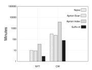
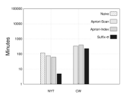
Figure 3: Wallclock times in minutes for (a) training a language model ($\sigma=5$, NYT: $\tau=10$ / CW: $\tau=100$) and (b) text analytics ($\sigma=100$, NYT: $\tau=100$ / CW: $\tau=1,000$) as two typical use cases

Figure 3 reports wallclock-time measurements obtained for these two use cases with 64 map/reduce slots. For our language-model use case, Suffix-$\sigma$ outperforms Apriori-Scan as the best competitor by a factor 3x on both datasets. For our analytics use case, we see a factor 12x improvement over Apriori-Index as the best competitor on NYT; on CW Suffix-$\sigma$ still outperforms the next best Apriori-Scan by a factor 1.5x. Measurements for Naïve on CW in are missing, since the method did not complete in reasonable time.

VII-E Varying Minimum Collection Frequency

Our second experiment studies how the methods behave as we vary the minimum collection frequency $\tau$. We use a maximum length $\sigma=5$ and apply all methods to the entire datasets. Measurements are performed using 64 map/reduce slots and reported in Figure 4.

NYT

(a) Wallclock times

(b) Bytes transferred

(c) # of records

(d) Wallclock times

(e) Bytes transferred

(f) # of records

CW

Figure 4: Varying the minimum collection frequency $\tau$

We observe that for high minimum collection frequencies, Suffix-$\sigma$ performs as well as the best competitor Apriori-Scan. For low minimum collection frequencies, it significantly outperforms the other methods. Both Apriori-based method show steep increases in wallclock time as we lower the minimum collection frequency – especially when we reach the lowest value of $\tau$ on each document collection. This is natural, because for both methods the work that has to be done in the $k$-th iteration depends on the number of $(k-1)$-grams output in the previous iteration, which have to be joined or kept in a dictionary, as described in Section III. As observed in Figure 2 above, the number of $k$-grams grows drastically as we decrease the value of $\tau$. When looking at the number of bytes and the number of records transferred, we see analogous behavior. For low values of $\tau$, Suffix-$\sigma$ transfers significantly less data than its competitors.

VII-F Varying Maximum Length

In this third experiment, we study the methods’ behavior as we vary the maximum length $\sigma$. The minimum collection frequency is set as $\tau=100$ for NYT and $\tau=1,000$ for CW to reflect their different scale. Measurements are performed on the entire datasets with 64 map/reduce slots and reported in Figure 5. Measurements for $\sigma>5$ are missing for Naïve on CW, since the method did not finish within reasonable time for those parameter settings.

NYT

(a) Wallclock times

(b) Bytes transferred

(c) # of records

(d) Wallclock times

(e) Bytes transferred

(f) # of records

CW

Figure 5: Varying the maximum length $\sigma$

Suffix-$\sigma$ is on par with the best-performing competitor on CW, when considering $n$-grams of length up to $50$. For $\sigma=100$, it outperforms the next best Apriori-Scan by a factor 1.5x. On NYT, Suffix-$\sigma$ consistently outperforms all competitors by a wide margin. When we increase the value of $\sigma$, the Apriori-based methods need to run more Hadoop jobs, so that their wallclock times keep increasing. For Naïve and Suffix-$\sigma$, on the other hand, we observe a saturation of wallclock times. This is expected, since these methods have to do additional work only for input sequences longer than $\sigma$ consisting of terms that occur at least $\tau$ times in the document collection. When looking at the number of bytes and the number of records transferred, we observe a saturation for Naïve for the reason mentioned above. For Suffix-$\sigma$ only the number of bytes saturates, the number of records transferred is constant, since it depends only on the minimum collection frequency $\tau$. Further, we see that Suffix-$\sigma$ consistently transfers fewest records.

VII-G Scaling the Datasets

Next, we investigate how the methods react to changes in the scale of the datasets. To this end, both from NYT and CW, we extract smaller datasets that contain a random $25\%$, $50\%$, or $75\%$ subset of the documents. Again, the minimum collection frequency is set as $\tau=100$ for NYT and $\tau=1,000$ for CW. The maximum length is set as $\sigma=5$. Wallclock times are measured using 64 map/reduce slots.

NYT                                           CW

(a) Wallclock times

(b) Wallclock times

Figure 6: Scaling the datasets

From Figure 6, we observe that Naïve handles additional data equally well on both datasets. The other methods’ scalability is comparable to that of Naïve on CW, as can be seen from their almost-identical slopes. On NYT, in contrast, Apriori-Scan, Apriori-Index, and Suffix-$\sigma$ cope slightly better with additional data than Naïve. This is due to the different characteristics of the two datasets.

VII-H Scaling Computational Resources

Our final experiment explores how the methods behave as we scale computational resources. Again, we set $\tau=100$ for NYT and $\tau=1,000$ for CW. All methods are applied to the $50\%$ samples of documents from the collections. We vary the number of map/reduce slots as 16, 32, 48, and 64. The number of cluster nodes remains constant in this experiment, since we cannot add/remove machines to/from the cluster due to organizational restrictions. We thus only vary the amount of parallel work every machine can do; their total number remains constant throughout this experiment.

NYT                                           CW

(a) Wallclock times

(b) Wallclock times

Figure 7: Scaling computational resources

We observe from Figure 7 that all methods show comparable behavior as we make additional computational resources available. Or, put differently, all methods make equally effective use of them. What can also be observed across all methods is that the gains of adding more computational resources are diminishing – because of mappers and reducers competing for shared devices such as hard disks and network interfaces. This phenomenon is more pronounced on NYT than CW, since methods take generally less time on the smaller dataset, so that competition for shared devices is fiercer and has no chance to level out over time.

Summary

What we see in our experiments is that Suffix-$\sigma$ outperforms its competitors when long and/or less frequent $n$-grams are considered. Even otherwise, when the focus is on short and/or very frequent $n$-grams, Suffix-$\sigma$ performs never significantly worse than the other methods. It is hence robust and can handle a wide variety of parameter choices. To substantiate this, consider that Suffix-$\sigma$ could compute statistics about arbitrary-length $n$-grams that occur at least five times (i.e., $\tau=5$ and $\sigma=\infty$), as reported in Figure 2, in less than six minutes on NYT and six hours on CW.

VIII Related Work

We now discuss the connection between this work and existing literature, which can broadly be categorized into:

Frequent Pattern Mining goes back to the seminal work by Agrawal et al. [8] on identifying frequent itemsets in customer transactions. While the Apriori algorithm described therein follows a candidate generation & pruning approach, Han et al. [20] have advocated pattern growth as an alternative approach. To identify frequent sequences, which is a problem closer to our work, the same kinds of approaches can be used. Agrawal and Srikant [10, 38] describe candidate generation & pruning approaches; Pei et al. [37] propose a pattern-growth approach. SPADE by Zaki [44] also generates and prunes candidates but operates on an index structure as opposed to the original data. Parallel methods for frequent pattern mining have been devised both for distributed-memory [19] and shared-memory machines [36, 45]. Little work exists that assumes MapReduce as a model of computation. Li et al. [26] describe a pattern-growth approach to mine frequent itemsets in MapReduce. Huang et al. [22] sketch an approach to maintain frequent sequences while sequences in the database evolve. Their approach is not applicable in our setting, since it expects input sequences to be aligned (e.g, based on time) and only supports document frequency. For more detailed discussions, we refer to Ceglar and Roddick [14] for frequent itemset mining, Mabroukeh and Ezeife [30] for frequent sequence mining, and Han et al. [21] for frequent pattern mining in general.

Natural Language Processing & Information Retrieval. Given their role in NLP, multiple efforts [11, 15, 18, 23, 39] have looked into $n$-gram statistics computation. While these approaches typically consider document collections of modest size, recently Lin et al. [27] and Nguyen et al. [34] targeted web-scale data. Among the aforementioned work, Huston et al. [23] is closest to ours, also focusing on less frequent $n$-grams and using a cluster of machines. However, they only consider $n$-grams consisting of up to eleven words and do not provide details on how their methods can be adapted to MapReduce. Yamamoto and Church [43] augment suffix arrays, so that the collection frequency of substrings in a document collection can be determined efficiently. Bernstein and Zobel [12] identify long $n$-grams as a means to spot co-derivative documents. Brants et al. [13] and Wang et al. [40] describe the $n$-gram statistics made available by Google and Microsoft, respectively. Zhai [46] gives details on the use of $n$-gram statistics in language models. Michel et al. [32] demonstrated recently that $n$-gram time series are powerful tools to understand the evolution of culture and language.

MapReduce Algorithms. Several efforts have looked into how specific problems can be solved using MapReduce, including all-pairs document similarity [28], processing relational joins [35], coverage problems [16], content matching [33]. However, no existing work has specifically addressed computing $n$-gram statistics in MapReduce.

IX Conclusions

In this work, we have presented Suffix-$\sigma$, a novel method to compute $n$-gram statistics using MapReduce as a platform for distributed data processing. Our evaluation on two real-world datasets demonstrated that Suffix-$\sigma$ outperforms MapReduce adaptations of Apriori-based methods significantly, in particular when long and/or less frequent $n$-grams are considered. Otherwise, Suffix-$\sigma$ is robust, performing at least on par with the best competitor. We also argued that our method is easier to implement than its competitors, having been designed with MapReduce in mind. Finally, we established our method’s versatility by showing that it can be extended to produce maximal/closed $n$-grams and perform aggregations beyond occurrence counting.

References

-
[1]
Apache Hadoop
http://hadoop.apache.org/. -
[2]
Apache OpenNLP
http://opennlp.apache.org/. -
[3]
Berkeley DB Java Edition
http://www.oracle.com/products/berkeleydb/. -
[4]
Boilerpipe
http://code.google.com/p/boilerpipe/. -
[5]
Google -Gram Corpus
http://googleresearch.blogspot.de/2006/08/
all-our-n-gram-are-belong-to-you.html. -
[6]
The ClueWeb09 Dataset
http://lemurproject.org/clueweb09. -
[7]