Redshifts, Sample Purity, and BCG Positions for the Galaxy Cluster Catalog from the first 720 Square Degrees of the South Pole Telescope Survey

Abstract

We present the results of the ground- and space-based optical and near-infrared (NIR) follow-up of 224 galaxy cluster candidates detected with the Sunyaev-Zel’dovich (SZ) effect in the 720 deg² of the South Pole Telescope (SPT) survey completed in the 2008 and 2009 observing seasons. We use the optical/NIR data to establish whether each candidate is associated with an overdensity of galaxies and to estimate the cluster redshift. Most photometric redshifts are derived through a combination of three different cluster redshift estimators using red-sequence galaxies, resulting in an accuracy of $\Delta z/(1+z)=0.017$, determined through comparison with a subsample of 57 clusters for which we have spectroscopic redshifts. We successfully measure redshifts for 158 systems and present redshift lower limits for the remaining candidates. The redshift distribution of the confirmed clusters extends to $z=1.35$ with a median of $z_{\mathrm{med}}=0.57$. Approximately 18% of the sample with measured redshifts lies at $z>0.8$. We estimate a lower limit to the purity of this SPT SZ-selected sample by assuming that all unconfirmed clusters are noise fluctuations in the SPT data. We show that the cumulative purity at detection significance $\xi>5$ ( $\xi>4.5$) is $\geq 95\%$ ($\geq 70\%$). We present the red brightest cluster galaxy (rBCG) positions for the sample and examine the offsets between the SPT candidate position and the rBCG. The radial distribution of offsets is similar to that seen in X-ray-selected cluster samples, providing no evidence that SZ-selected cluster samples include a different fraction of recent mergers than X-ray-selected cluster samples.

1. Introduction

In November 2011, the South Pole Telescope (SPT; Carlstrom et al., 2011) collaboration completed a 2500 $\mathrm{deg}^{2}$ survey, primarily aimed at detecting distant, massive galaxy clusters through their Sunyaev-Zel’dovich (SZ) effect signature. In Reichardt et al. (2012, R12 hereafter), the SPT team presented a catalog of 224 cluster candidates from 720 $\mathrm{deg}^{2}$ observed in the 2008-2009 seasons. In this work, we present the optical and near-infrared (NIR) follow-up observations of the cluster candidates reported in R12, mainly focusing on follow-up strategy, confirmation and empirical purity estimate for the cluster candidates, photometric redshift estimations of confirmed clusters, and the spatial position of the red brightest cluster galaxies.

Galaxy clusters have long been used for the study of structure formation and cosmology (e.g., Geller & Beers, 1982; White et al., 1993). Soon after the discovery of the cosmic acceleration (Schmidt et al., 1998; Perlmutter et al., 1999), it became clear that measurements of the redshift evolution of the cluster mass function could provide a powerful tool to further understand the underlying causes (Wang & Steinhardt, 1998; Haiman et al., 2001; Holder et al., 2001; Battye & Weller, 2003). More precise theoretical investigations (Majumdar & Mohr, 2003; Hu, 2003; Majumdar & Mohr, 2004; Molnar et al., 2004; Wang et al., 2004; Lima & Hu, 2005, 2007) identified the key challenges associated with cluster surveys, which include: (1) producing large uncontaminated samples selected by an observable property that is closely related to the cluster mass, (2) measuring cluster redshifts for large samples and (3) precisely calibrating the cluster masses.

Competitive approaches to producing large cluster samples include optical multiband surveys (e.g., Gladders & Yee, 2005; Koester et al., 2007), infrared surveys (e.g., Eisenhardt et al., 2008; Muzzin et al., 2008; Papovich, 2008), X-ray surveys (e.g., Finoguenov et al., 2007; Pacaud et al., 2007; Vikhlinin et al., 2009; Finoguenov et al., 2010; Mantz et al., 2010; Fassbender et al., 2011; Lloyd-Davies et al., 2011; Šuhada et al., 2012), and millimeter-wave (mm-wave) surveys (Vanderlinde et al., 2010; Marriage et al., 2011; Planck Collaboration et al., 2011; Reichardt et al., 2012). The mm-wave surveys capitalize on the cluster SZ effect signature, which is produced by the inverse Compton scattering of cosmic microwave background photons by the energetic electrons within the cluster (Sunyaev & Zel’dovich, 1972). The surface brightness of the SZ effect is redshift-independent, making SZ surveys a particularly powerful tool for identifying the most distant clusters. It is typical for X-ray and mm-wave surveys to have accompanying multiband optical imaging to enable photometric redshift measurements; these multiband optical data also enable a second stage of cluster candidate confirmation, verifying the purity estimation of the X-ray or SZ-selected cluster samples.

Ideally, one would coordinate an SZ survey with a deep, multiband optical survey over the same region; indeed, the Dark Energy Survey (DES; Cease et al., 2008; Mohr et al., 2008) and the SPT are coordinated in this way. Because of the different development timelines for the two projects, it has been necessary to undertake extensive cluster-by-cluster imaging follow-up for SPT using a series of ground-based telescopes together with space-based NIR imaging (from Spitzer and WISE). The NIR data are of particular importance in the confirmation and redshift estimation of the $z>1$ massive galaxy clusters, which are especially interesting for both cosmological studies and studies of the evolution of clusters themselves. Pointed observations were used in High et al. (2010, H10 hereafter) to provide redshift and richness estimates of the SZ detections of Vanderlinde et al. (2010), and subsequently by Williamson et al. (2011) and Story et al. (2011).

Cluster samples from high-resolution SZ surveys can be also used to explore the evolution of cluster properties as a function of redshift. Previous studies using X-ray-selected clusters have identified a correlation between the dynamical state of a cluster and the projected offset between the X-ray centers and the brightest cluster galaxy (e.g., Katayama et al., 2003; Sanderson et al., 2009; Haarsma et al., 2010; Fassbender et al., 2011; Stott et al., 2012). In principle, SZ-selected clusters can serve as laboratories to search for this correlation also, if the spatial resolution of SZ detections is high enough to detect the significance of offsets between the SZ centers and the brightest cluster galaxies. Systematic comparison between X-ray and SZ samples will indicate if the selection of the two methods differs in terms of the dynamical state of clusters.

This paper is structured as follows: we briefly describe the SPT data and methods for extracting the cluster sample in §2.1. In §2.2, we provide details of the follow-up strategy, as well as data processing. §3 is dedicated to a detailed description of the analysis of our follow-up data, including redshift estimation using optical and Spitzer data, the derivation of redshift lower limits for those systems that are not confirmed, and the selection of red brightest cluster galaxies (rBCGs) in the clusters. Results are presented in §4 and discussed further in §5. Throughout this paper, we use the AB magnitude system for optical and NIR observations unless otherwise noted in the text.

2. Discovery & Followup

2.1. SPT Data

Here we briefly summarize the analysis of the SPT data and the extraction of cluster candidates from that data; we refer the reader to R12 and previous SPT cluster publications (Staniszewski et al., 2009; Vanderlinde et al., 2010; Williamson et al., 2011) for more details.

The SPT operates in three frequency bands, although only data from the 95 GHz and 150 GHz detectors were used in finding clusters. The data from all detectors at a given observing frequency during an observing period (usually 1-2 hours) are combined into a single map. The data undergo quality cuts and are high-pass filtered and inverse-noise-weighted before being combined into a map. Many individual-observation maps of every field are co-added (again using inverse noise weighting) into a full-depth map of that field, and the individual-observation maps are differenced to estimate the map noise. The 95 GHz and 150 GHz full-depth maps of a given field are then combined using a spatial-spectral matched filter (e.g., Melin et al., 2006) that optimizes signal-to-noise on cluster-shaped objects with an SZ spectral signature. Cluster candidates are identified in the resulting filtered map using a simple peak detection algorithm, and each candidate is assigned a signal-to-noise value based on the peak amplitude divided by the RMS of the filtered map in the neighborhood of the peak. Twelve different matched filters are used, each assuming a different scale radius for the cluster, and the maximum signal-to-noise for a given candidate across all filter scales is referred to as $\xi$, which we use as our primary SZ observable. In 2008, the 95 GHz detectors in the SPT receiver had significantly lower sensitivity than the 150 GHz array, and the cluster candidates from those observations are identified using 150 GHz data only; the candidates from 2009 observations were identified using data from both bands. The data from the two observing seasons yielded a total of 224 cluster candidates with $\xi$$\geq$$4.5$—the sample discussed here.

2.2. Optical/NIR Imaging

The cluster candidates detected using the method described above are followed up by optical and, in many cases, NIR instruments. In this section, we describe the overall optical/NIR follow-up strategy, the different imaging and spectroscopic observations and facilities used, and the data reduction methods used to process the raw images to catalogs.

2.2.1 Imaging Observations

The optical/NIR follow-up strategy has evolved since the first SPT-SZ candidates were identified. Originally we imaged regions of the sky with uniformly deep, multiband observations in $griz$ optical bands to confirm SZ detections and estimate redshifts as in Staniszewski et al. (2009). For the first SPT cluster candidates, we used imaging from the Blanco Cosmology Survey (BCS; Desai et al., 2012) to follow up candidates in parts of the 2008 fields. The BCS is a 60-night, $\sim$$80$ $\mathrm{deg}^{2}$ NOAO survey program carried out in 2005-2008 using the Blanco/MOSAIC2 $griz$ filters. The BCS survey was completed to the required depths for $5\sigma$ detection at $0.4L^{*}$ within $2\farcs 3$ apertures up to $z$$\sim$$1$. The goal of this survey was to provide optical imaging over a limited area of the SPT survey to enable rapid optical follow-up of the initial SPT survey fields.

For clusters outside the BCS region we initially obtained deep $griz$ imaging on a cluster-by-cluster basis. But as the SPT survey proceeded and the cluster candidate list grew, it became clear that this strategy was too costly, given the limited access to follow-up time. Moreover, eventually the full SPT region will be imaged to uniform 10$\sigma$ depths of mag$\sim$24 in $griz$ by the DES. We therefore switched to an adaptive strategy of follow-up in which we observed each SPT cluster candidate to the depth required to find an optical counterpart and determine its redshift.

For each SPT cluster candidate, we perform an initial pre-screening of candidates using the Digitized Sky Survey (DSS). We examine DSS images using 3 bands for each cluster candidate to determine whether it is “low-$z$” or “high-$z$,” where the redshift boundary lies roughly at $z=0.5$. We find that this visual classification identifies spectroscopically and photometrically confirmed SPT clusters out to $z$=0.5 in the DSS photographic plates. We use the DSS designation to prioritize the target list for the appropriate telescope, instrument and filters with which we observe each candidate. Specifically, candidates that are clearly identified in DSS images are likely to be low-$z$ clusters and are designated for follow-up observations on small-aperture (1m-2m) telescopes. Otherwise, candidates are classified as high-$z$ candidates and therefore designated for large-aperture (4m-6.5m) telescopes. The various ground- and space-based facilities used to collect optical/NIR imaging data on SPT clusters are summarized in Table 1. Each telescope/instrument combination is assigned a numeric alias that is used to identify the source of the redshift data for each cluster in Table A.

For the $\geq 4$m-class observations, we use an adaptive filter and exposure time strategy so that we can efficiently bracket the cluster member galaxy’s 4000Å break to the depth required for redshift estimation. In this approach we start with a first imaging pass, where each candidate is observed in the $g$, $r$, and $z$ bands to achieve a depth corresponding to a $5\sigma$ detection of a $0.4L^{*}$ galaxy at $z=0.8$, $\sim$23.5 mag and 21.8 mag in $r$ and $z$ bands respectively, based on the Bruzual & Charlot (2003) red-sequence model (for more details about the model, see § 3.1). Observations are also taken in a single blue filter for photometric calibration using the stellar locus (discussed in §2.2.2). For candidates with no obvious optical counterpart after first-pass observations, a second-pass is executed to get to $z=$ 0.9, $\sim$23 mag and 22 mag in $i$ and $z$ bands respectively.

If the candidate is still not confirmed after the second-pass in $i$ and $z$ bands, and is not covered by the Spitzer/IRAC pointed observations described below, we attempt to obtain ground-based NIR imaging for that candidate using the NEWFIRM camera on the CTIO Blanco telescope. The data presented here are imaged with NEWFIRM during three observing runs in 2010 and 2011, yielding $K_{s}$ data for a total of 31 candidates. Typical observations in $K_{s}$ consist of 16 point dither patterns, with 60 second exposures divided among 6 coadds at each dither position. Median seeing during the 2010 runs was 1$\farcs$05; during the 2011 run observing conditions were highly variable and the seeing ranged from $1\farcs 05$ to 2$\farcs 6$ with median seeing $\sim 1\farcs 2$.

We note that most of the galaxy cluster candidates in this work with significance $\xi>4.8$ were imaged with Spitzer (Werner et al., 2004). More specifically, Spitzer/IRAC (Fazio et al., 2004) imaging has been obtained for 99 SZ cluster candidates in this work. The on-target Spitzer observations consist of 8$\times 100$ s and 6$\times 30$ s dithered exposures at 3.6$\mu$m and 4.5$\mu$m, respectively. The deep 3.6$\mu$m observations should produce $5\sigma$ detections of passively-evolving $0.1L^{*}$ cluster galaxies at $z=1.5$ ($\sim$17.8 mag (Vega) at $z=1.5$).

For some of the NIR analysis, we augment the data from our Spitzer and NEWFIRM observations with the recently released all-sky Wide-field Infrared Survey Explorer (WISE; Wright et al., 2010) data. Finally, we note that a few of the clusters were observed with Magellan/Megacam to obtain weak gravitational lensing mass measurements (High et al., 2012). These data are naturally much deeper than our initial followup imaging.

Table 1Optical and infrared imagers

Ref.	Site	Telescope	Aperture	Camera	Filters	Field	Pixel scale
			(m)				($\arcsec$)
1	Cerro Tololo	Blanco	4	MOSAIC-II	$griz$	$36\arcmin\times 36\arcmin$	$0.27$
2	Las Campanas	Magellan/Baade	6.5	IMACS f/2	$griz$	$27\farcm 4\times 27\farcm 4$	$0.200$
3	Las Campanas	Magellan/Clay	6.5	LDSS3	$griz$	$8\farcm 3$ diam. circle	$0.189$
4	Las Campanas	Magellan/Clay	6.5	Megacam	$gri$	$25\arcmin\times 25\arcmin$	$0.16$
5	Las Campanas	Swope	1	SITe3	$BVRI$	$14\farcm 8\times 22\farcm 8$	$0.435$
6	Cerro Tololo	Blanco	4	NEWFIRM	$K_{s}$	$28\arcmin\times 28\arcmin$	$0.4$
7	$\cdots$	Spitzer Space Telescope	0.85	IRAC	3.6$\mu$m, 4.5$\mu$m	$5\farcm 2\times 5\farcm 2$	$1.2$
8	$\cdots$	Wide-field Infrared Survey Explorer	0.40	$\cdots$	3.4$\mu$m, 4.6$\mu$m	$47\arcmin\times 47\arcmin$	$6$

Note. — Optical and infrared cameras used in SPT follow-up observations.

2.2.2 Data Processing

We use two independent optical data processing systems. One system, which we refer to as the PHOTPIPE pipeline, is used to process all optical data except Magellan/Megacam data, and the other, which is a development version of the Dark Energy Survey data management (DESDM) system, is used only to process the Blanco/Mosaic2 data. PHOTPIPE was used to process optical data for previous SPT cluster catalogs (Vanderlinde et al., 2010; High et al., 2010; Williamson et al., 2011); the DESDM system has been used as a cross-check in these works and was the primary reduction pipeline used in Staniszewski et al. (2009).

The basic stages of the PHOTPIPE pipeline, initially developed for the SuperMACHO and ESSENCE projects and described in Rest et al. (2005), Garg et al. (2007), and Miknaitis et al. (2007), include flat-fielding, astrometry, coadding, and source extraction. Further details are given in H10. In the DESDM system (Ngeow et al., 2006; Mohr et al., 2008; Desai et al., 2012), the data from each night first undergo detrending corrections, which include cross-talk correction, overscan correction, trimming, bias subtraction, flat fielding and illumination correction. Single epoch images are not remapped to avoid correlating noise, and so we also perform a pixel-scale correction that brings all sources on an image to a common photometric zeropoint. For $i$ and $z$ bands we also carry out a fringe correction. Astrometric calibration is done by using the AstrOmatic code SCAMP (Bertin, 2006) and the USNO-B catalog. Color terms to transform to the SDSS system rely on photometric solutions derived from observations of SDSS equatorial fields during photometric nights (Desai et al., 2012).

In both pipelines, coaddition is done using SWarp (Bertin et al., 2002). In the DESDM system the single epoch images contributing to the coadd are brought to a common zeropoint using stellar sources common to pairs of images. The final photometric calibration of the coadd images is carried out using the stellar color-color locus as a constraint on the zeropoint offsets between neighboring bands (e.g., High et al., 2009), where the absolute photometric calibration comes from 2MASS (Skrutskie et al., 2006). For $griz$ photometry the calibration is done with reference to the median SDSS stellar locus (Covey et al., 2007), but for the Swope data using Johnson filters, the calibration relies on a stellar locus derived from a sequence of models of stellar atmospheres from PHOENIX (Brott & Hauschildt, 2005) with empirically measured CCD, filter, and atmosphere responses. Cataloging is done using SExtractor (Bertin & Arnouts, 1996), and within the DESDM catalogs we calibrate mag_auto using stellar locus.

Quality checks of the photometry are carried out on a cluster by cluster basis using the scatter of stars about the expected stellar locus and the distribution of offsets in the single-epoch photometry as a function of calibrated magnitude (so-called photometric repeatability tests). Poor quality data or failed calibrations are easily identified as those coadds with high stellar locus scatter and or high scatter in the photometric repeatability tests (see Desai et al., 2012).

NEWFIRM imaging data are reduced using the FATBOY pipeline (Eikenberry et al., 2006), originally developed for the FLAMINGOS-2 instrument, and modified to work with NEWFIRM data in support of the Infrared Bootes Imaging Survey (Gonzalez et al., 2010). Individual processed frames are combined using SCAMP and SWarp, and photometry is calibrated to 2MASS.

Spitzer/IRAC data are reduced following the method of Ashby et al. (2009). Briefly, we correct for column pulldown, mosaic the individual exposures, resample to 0$\farcs$86 pixels (half the solid angle of the native IRAC pixels), and reject cosmic rays. Magnitudes are measured in 4″–diameter apertures and corrected for the 38% and 40% loss at 3.6$\mu$m and 4.5$\mu$m respectively due to the broad PSF (see Table 3 in Ashby et al., 2009). The Spitzer photometry is crucial to the measurement of photometric redshifts for clusters at $z\gtrsim 0.8$, as described in §3.1.

The acquisition and processing for the initial weak lensing Megacam data is described in detail in High et al. (2012). These data are reduced separately from the other imaging data using the Smithsonian Astrophysical Observatory (SAO) Megacam reduction pipeline. Standard raw CCD image processing, cosmic-ray removal, and flat-fielding are performed, as well as an additional illumination correction to account for a low-order scattered light pattern. The final images are coadded onto a single pixel grid with a pixel scale of $0\farcs 16$ using SWarp. Sources are detected in the coadded data in dual-image mode using SExtractor, where the $r$ band image serves as the detection image. The photometry is calibrated by fitting colors to the stellar locus, and color-term corrections are accounted for in this step. The color term is roughly $0.10(g-i)$ for the $g^{\prime}$ band, $-0.02(g-i)$ for the $r^{\prime}$ band, and $-0.03(g-i)$ for the $i^{\prime}$ band.

2.3. Spectroscopic Observations

We have targeted many of the SPT clusters with long-slit and multi-object spectroscopy, and some of the spectroscopic redshifts have appeared in previous SPT publications. We have used a variety of instruments: GMOS-S on Gemini South, FORS2 (Appenzeller et al., 1998) on VLT, LDSS3 on Magellan-Clay, and the IMACS camera on Magellan Baade (in long-slit mode and with the GISMO complement).

A detailed description of the configurations, observing runs and reductions will be presented elsewhere (J. Ruel et al., in prep). For a given cluster we target bright galaxies that lie on the clusters’ red sequence and observe these galaxies with a combination of filter and disperser that yields a low-resolution spectrum around their Ca II H&K lines and 4000Å break. CCD reductions are made using standard packages, including COSMOS (Kelson, 2003) for IMACS data and IRAF for GMOS and FORS2. Redshift measurements are made by cross-correlation with the RVSAO package (Kurtz & Mink, 1998) and a proprietary template fitting method that uses SDSS DR2 templates. Results are then visually confirmed using strong spectral features.

In Table 2, the source for every spectroscopic redshift is listed, along with the number of cluster members used in deriving the redshift. For clusters for which we report our own spectroscopic measurements, we list an instrument name and observation date; we give a literature reference for those for which we report a value from the literature. In Table A, we report spectroscopic redshifts for 57 clusters, of which 36 had no previous spectroscopic redshift in the literature. Unless otherwise noted, the reported cluster redshift is the robust biweight average of the redshifts of all spectroscopically confirmed cluster members, and the cluster redshift uncertainty is found from bootstrap resampling.

Table 2Spectroscopic Follow-Up

Cluster	Inst	Obs	#	Refs	Cluster	Inst	Obs	#	Refs
SPT-CLJ0000-5748	GMOS-S	Sep 2010	26	–	SPT-CLJ2058-5608	GMOS-S	Sep 2011	9	–
SPT-CLJ0205-5829	IMACS	Sep 2011	9	a	SPT-CLJ2100-4548	FORS2	Aug 2011	19	–
SPT-CLJ0205-6432	GMOS-S	Sep 2011	15		SPT-CLJ2104-5224	FORS2	Jun 2011	23	–
SPT-CLJ0233-5819	GMOS-S	Sep 2011	10		SPT-CLJ2106-5844	FORS2	Dec 2010	15	–
SPT-CLJ0234-5831	GISMO	Oct 2010	22	b		GISMO	Jun 2010	3	i
SPT-CLJ0240-5946	GISMO	Oct 2010	25	–	SPT-CLJ2118-5055	FORS2	May 2011	25	–
SPT-CLJ0254-5857	GISMO	Oct 2010	35	b	SPT-CLJ2124-6124	GISMO	Sep 2009	24	–
SPT-CLJ0257-5732	GISMO	Oct 2010	22	–	SPT-CLJ2130-6458	GISMO	Sep 2009	47	–
SPT-CLJ0317-5935	GISMO	Oct 2010	17	–	SPT-CLJ2135-5726	GISMO	Sep 2010	33	–
SPT-CLJ0328-5541	–	–	–	c	SPT-CLJ2136-4704	GMOS-S	Sep 2011	24	–
SPT-CLJ0431-6126	–	–	–	c	SPT-CLJ2136-6307	GISMO	Aug 2010	10	–
SPT-CLJ0433-5630	GISMO	Jan 2011	22	–	SPT-CLJ2138-6007	GISMO	Sep 2010	34	–
SPT-CLJ0509-5342	GMOS-S	Dec 2009	18	d, e	SPT-CLJ2145-5644	GISMO	Sep 2009	37	–
SPT-CLJ0511-5154	GMOS-S	Sep 2011	15	–	SPT-CLJ2146-4633	IMACS	Sep 2011	17	–
SPT-CLJ0516-5430	GISMO	Sep 2010	48	f	SPT-CLJ2146-4846	GMOS-S	Sep 2011	26	–
SPT-CLJ0521-5104	–	–	–	e	SPT-CLJ2148-6116	GISMO	Sep 2009	30	–
SPT-CLJ0528-5300	GMOS-S	Jan 2010	20	d, e	SPT-CLJ2155-6048	GMOS-S	Sep 2011	25	–
SPT-CLJ0533-5005	LDSS3	Dec 2008	4	d	SPT-CLJ2201-5956	–	–	–	c
SPT-CLJ0534-5937	LDSS3	Dec 2008	3	–	SPT-CLJ2300-5331	GISMO	Oct 2010	24	–
SPT-CLJ0546-5345	GISMO	Feb 2010	21	g	SPT-CLJ2301-5546	GISMO	Aug 2010	11	–
	GMOS-S	Dec 2009	2	e	SPT-CLJ2331-5051	GMOS-S	Aug 2010	28	–
SPT-CLJ0551-5709	GISMO	Sep 2010	34	d		GISMO		50	d
SPT-CLJ0559-5249	GMOS-S	Nov 2009	37	d, e	SPT-CLJ2332-5358	GISMO	Jul 2009	24	–
SPT-CLJ2011-5725	–	–	–	f	SPT-CLJ2337-5942	GMOS-S	Aug 2010	19	d
SPT-CLJ2012-5649	–	–	–	c	SPT-CLJ2341-5119	GMOS-S	Aug 2010	15	d
SPT-CLJ2022-6323	GISMO	Oct 2010	37	–	SPT-CLJ2342-5411	GMOS-S	Sep 2010	11	–
SPT-CLJ2023-5535	–	–	–	f	SPT-CLJ2351-5452	–	–	–	h
SPT-CLJ2032-5627	GISMO	Oct 2010	31	–	SPT-CLJ2355-5056	GISMO	Sep 2010	37	–
SPT-CLJ2040-5725	GISMO	Aug 2010	5	–	SPT-CLJ2359-5009	GISMO	Aug 2010	21	–
SPT-CLJ2043-5035	FORS2	Aug 2011	21	–		GMOS-S	Dec 2009	9	–
SPT-CLJ2056-5459	GISMO	Aug 2010	12	–

Note. — Instruments [Inst] : GMOS-S on Gemini South 8m, IMACS on Magellan Baade 6.5m, GISMO complement to IMACS on Magellan Baade 6.5m, LDSS3 on Magellan Clay 6.5, FORS2 on VLT Antu 8m; Observing dates [Obs]: dates each data taken; Number of galaxies [#]: Number of galaxies used in deriving redshifts; References [Refs]: ^aStalder et al. (2012), ^bWilliamson et al. (2011), ^cStruble & Rood (1999), ^dHigh et al. (2010), ^eSifon et al. (2012), ^fBöhringer et al. (2004), ^gBrodwin et al. (2010), ^hBuckley-Geer et al. (2011), ⁱFoley et al. (2011)

3. Methodology

In this section, we describe the analysis methods used to: 1) extract cluster redshift estimates and place redshift limits; 2) empirically verify the estimates of catalog purity; and 3) measure rBCG positions.

3.1. Photometric Redshifts

Using the procedure described in §2.2, we obtain ground-based imaging data and galaxy catalogs that in most cases allow us to identify an obvious overdensity of red-sequence galaxies within approximately an arcminute of the SPT candidate position. For these optically confirmed cluster candidates, we proceed to estimate a photometric redshift.

In this work, we employ three methods (which we refer to Method 1, 2, and 3 in the following sections) to estimate cluster redshifts from optical imaging data. Two methods (Method 1 and 2) use the color of the galaxies in the cluster red sequence, and the third (Method 3) uses the average of red-sequence galaxy photometric redshifts estimated with a neural-network algorithm, trained with the magnitudes of similar galaxies. In the optical analysis for our two previous cluster catalog releases (High et al., 2010; Williamson et al., 2011), we relied on Method 1 for the results and Method 3 as a cross-check. In this work, we improve the precision of the measured redshifts by applying multiple redshift estimation algorithms and combining the results. Through cross-checks during the analysis, we find that these methods have different failure modes and that comparing the results provides a way of identifying systems that require additional attention (including systems where the cluster’s central region is contaminated by foreground stars or the cluster resides in a crowded field).

All three methods use the single-stellar-population (SSP) models of Bruzual & Charlot (BC03; 2003). These models allow us to transform the location of the red-sequence overdensity in color space to a redshift estimate. A model for the red galaxy population as a function of redshift is built assuming a single burst of star formation at $z_{f}=3$ followed by passive evolution thereafter. Models are selected over a range of metallicities and then calibrated to reproduce the color and tilt of the red sequence in the Coma cluster (Eisenhardt et al., 2007) at $z=0.023$. The calibration procedure is described in more detail in Song et al. (2012). The red sequence model prescribed in a similar way has been demonstrated to adequately describe the bright end of the cluster red sequence (Blakeslee et al., 2003; Tran et al., 2007; Muzzin et al., 2009; High et al., 2010; Mancone et al., 2010; Stott et al., 2010; Song et al., 2012). These models are used in determining exposure times and appropriate filter combinations for imaging observations, and in the calculation of redshifts and redshift limits from those observations.

3.1.1 Photometric Redshift Measurement Methods

In Method 1, a cluster is confirmed by identifying an excess of galaxies with colors consistent with those derived from BC03 (simultaneously for all observed filters), after subtracting the background surface density. The background-subtracted galaxy number is extracted from an aperture within a radius of (3.5,2.5,1.5)^′ from the SPT candidate position and uses galaxies with photometric color uncertainties $\leq$(0.25,0.35,0.45) and apparent magnitudes brighter than $m^{*}$+(3,2,1) (or the magnitude limit of the data) in the red sequence based on the same BC03 models, for $z$$<$$0.2$, $0.2$$<$$z$$<0.6$, and $z$$>$$0.6$ respectively. The background measurement is obtained by applying the same criteria outside of the cluster search aperture. The redshift is estimated from the most significant peak in this red-sequence galaxy excess. Improvements over the implementation in H10 include using additional colors ($r$-$z$ and $g$-$i$, plus NIR colors) in the red-sequence fitting, using the deeper photometry available from coadded images, and sampling the entire CCD mosaic rather than a single CCD for better background estimation.

Method 2 is similar in that it searches for an overdensity of red-sequence galaxies. This method, used to estimate the redshifts for a sample of 46 X-ray-selected clusters (Šuhada et al., 2012), is described and tested in more detail in Song et al. (2012). It includes a measure of the background surface density based on the entire imaged sky area surrounding each cluster candidate and subtracts the background from the red galaxy counts in an aperture of 0.8 Mpc. Only galaxies with luminosity $>0.4$L^∗ and magnitude uncertainty $\leq 0.25$ are used, and the aperture and luminosity are recalculated for each potential redshift. Originally as described in Song et al. (2012), we search for an overdensity of red-sequence galaxies using two or three available color-redshift combinations simultaneously for every cluster; essentially, we scan outwards in redshift using the following color combinations: $g$-$r$ and $g$-$i$ for $z<$$0.35$, $g$-$i$ and $r$-$i$ and $r$-$z$ for $0.3$$<$$z$$<$$0.75$, $r$-$z$ and $i$-$z$ for $z$$>$$0.75$. The cluster photometric redshift is extracted from the peak of the galaxy overdensity in redshift space. The redshift is then refined by fitting the red-sequence overdensity distribution in redshift space with a Gaussian function. The version used here (which is the same as the method used in Šuhada et al. 2012) has one more refinement, in which the colors of the galaxies that lie in the peak redshift bin identified by the overdensity method are converted into individual galaxy photometric redshifts. In this conversion we assume that the galaxies are red-sequence cluster member galaxies, and the photometric redshift uncertainty reflects the individual photometric color errors. A final cluster redshift is calculated as an inverse-variance-weighted mean of these galaxy photometric redshifts.

Method 3 shares the same principle as the other two in that it involves searching for a density peak in the galaxy distribution near the position of the SPT candidate. We first select individual red cluster members using location relative to the SPT candidate position and galaxy color as the criteria for cluster membership. For the redshifts presented here, this is done visually using pseudo-color coadded images for each cluster, although in principle this could be automated. Galaxy selection is not confined by a specific radial distance from SZ centers as in the other two methods, nor by photometric uncertainties. Selected galaxies are then fed into Artificial Neural Networks (ANN$z$; Collister & Lahav, 2004), which is trained using the same BC03 models used in the other methods. ANN$z$ returns redshift estimates for individual galaxies, and a peak in galaxy redshift distribution is adopted as the initial cluster redshift. Then, as in Method 2, individual galaxy photometric redshifts are averaged using inverse-variance weighting to produce the cluster photometric redshift. With this initial estimate of the redshift, we then perform an outlier rejection using iterative $1\sigma$ clipping, where the $1\sigma$ corresponds to the root-mean-square (RMS) variation of the measured galaxy photometric redshift distribution. Once the rejection is carried out, we refine the cluster photometric redshift estimate using the weighted mean of the non-rejected sample of cluster galaxies. No outlier rejection is undertaken if there are fewer than 20 selected galaxies in the original sample.

Method 3 is a good cross-check, as well as a stand-alone redshift estimator, because we can visually confirm which galaxies contribute to the redshift determination. Although this method requires photometry in more than just two bands, it appears to be less susceptible to the problems in two-band methods that are associated with pileup of red sequence galaxies at redshifts where the 4000Å  break is transitioning out of a band.

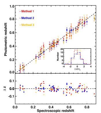
Figure 1.— $\it{Top}$: Photometric redshift $z_{\mathrm{phot}}$ versus spectroscopic redshift $z_{\mathrm{spec}}$  for each redshift estimation method for 47 spectroscopically confirmed clusters at $z<0.9$ where we use only $griz$ photometry. $\it{Bottom}$: the distribution of the photometric redshift residuals $\Delta z=z_{\mathrm{phot}}-z_{\mathrm{spec}}$ as a function of $z_{\mathrm{spec}}$. $\it{Inset}$: the normalized residual distributions, which all have $RMS(\Delta z/\sigma_{z_{\mathrm{phot}}})\sim 1$. The RMS scatter of $\Delta z/(1+z)$ is 0.028, 0.023 and 0.024 for Methods 1 (red dot and red dashed line), 2 (blue square and blue dash-dot-dot line) and 3 (yellow triangle and yellow dotted line), respectively.

Next we characterize redshift estimates from each method using spectroscopically confirmed clusters. We use 47 clusters with spectroscopic redshifts ($z_{\mathrm{spec}}$) where only $griz$ data are used for photometric redshift estimation. In this process, photometric redshift ($z_{\mathrm{phot}}$) biases (namely, smooth trends of photometric redshift offset as a function of redshift) are measured and corrected in Method 1 and 2, while no significant bias correction is necessary for Method 3. Bias corrections depend on several factors, such as filters used for data, redshift of clusters, and the depth of the data. They are separately measured in those different cases per method as a function of (1+$z$) at a level of 0.01-0.03 in redshift for clusters with redshift measured in $griz$ filters, Spitzer-only, and $BVRI$ filters at $z>0.5$. The largest bias correction is needed for clusters observed from SWOPE using $BVRI$ filters with maximum correction of 0.13 at around $z\sim 0.4$ where the filter transitions from $B$-$V$ to $V$-$R$ occurs to capture the red sequence population. This affects two clusters in the final sample. Once biases are removed, we examine the photometric-to-spectroscopic redshift offsets to characterize the performance of each method. We find the RMS in the quantity $\Delta z$/(1+$z_{\mathrm{spec}}$), where $\Delta z=z_{\mathrm{phot}}-z_{\mathrm{spec}}$ to have values of 0.028, 0.023, and 0.024 in Methods 1, 2, and 3, respectively (see Figure 1). We note that some of the bias and systematic error, especially at higher redshift, could be due to the mismatch between the SEDs in the red sequence model and the cluster population, which could arise from variations in star formation history or AGN activity.

Our goal is not only to estimate accurate and precise cluster redshifts, but also to accurately characterize the uncertainty in these estimates. To this end, we use the spectroscopic subsample of clusters to estimate a systematic floor $\sigma_{\mathrm{sys}}$ in addition to the statistical component. We do this by requiring that the reduced $\chi^{2}$ describing the normalized photometric redshift deviations from the true redshifts $\chi^{2}_{\mathrm{red}}=\sum(\Delta z/\sigma_{z_{\mathrm{phot}}})^{2}/N_{\mathrm{dof}}$ have a value $\chi^{2}_{\mathrm{red}}\sim 1$ for each method, where $\sigma_{z_{\mathrm{phot}}}$ is the uncertainty in measured $z_{\mathrm{phot}}$ and $N_{\mathrm{dof}}$ is the number of degrees of freedom. We adopt uncertainties $\sigma_{z_{\mathrm{phot}}}^{2}=\sigma_{\mathrm{stat}}^{2}+\sigma_{\mathrm{sys}}^{2}$ and adjust $\sigma_{\mathrm{sys}}$ to obtain the correct $\chi^{2}_{\mathrm{red}}$. In this tuning process we also include redshift estimates of the same cluster from multiple instruments when that cluster has been observed multiple times. This allows us to test the performance of our uncertainties over a broader range of observing modes and depths than is possible if we just use the best available data for each cluster.

For Method 1 we separately measure the systematic floor $\sigma_{\mathrm{sys}}$ for each different photometric band set. For the $grizK_{S}$ instruments (Megacam, IMACS, LDSS3, MOSAIC2, NEWFIRM), we estimate $\sigma_{\mathrm{sys}}=0.039$ ; for the $BVRI$ instrument (Swope), $\sigma_{\mathrm{sys}}=0.033$; and for Spitzer-only, $\sigma_{\mathrm{sys}}=0.070$. In Method 2, we find $\sigma_{\mathrm{sys}}=0.030$ for the $griz$ instruments (Megacam, IMACS, LDSS3, MOSAIC2). For Method 3 we estimate $\sigma_{\mathrm{sys}}=0.028$ for the $griz$ instruments.

Once this individual estimation and calibration is done, we conduct an additional test on the redshift estimation methods, again using the spectroscopic subsample. The purpose of this test is to see how the quality of photometry (i.e., follow-up depth) affects the estimations. We divide the spectroscopic sample into two groups: in one group, the photometric data is kept at full depth, while the photometric data in the other group is manually degraded to resemble the data from the shallowest observations in the total follow-up sample. To create the ‘shallow’ catalogs, we add white noise to the full-depth coadds and then extract and calibrate catalogs from these artificially noisier images. Results of this test show that the accuracy of the photometric redshift estimation is affected by the poorer photometry, but that this trend is well captured by the statistical uncertainties in each estimation method.

3.1.2 Combining Photo-z Estimates to Obtain $z_{\mathrm{comb}}$

Once redshifts and redshift uncertainties are estimated with each method independently, we compare the different redshift estimates of the same cluster. Note that this comparison is not possible for Swope or Spitzer-only redshifts, which are measured only with Method 1. Outliers at $\geq 3\sigma$ ($>$6%) in 1+$z_{\mathrm{phot}}$ are identified for additional inspection. In some cases, there is an easily identifiable and correctable issue with one of the methods, such as misidentification of cluster members. If, however, it is not possible to identify an obvious problem, the outliers are excluded from the combining procedure. This outlier rejection, which occurs only in two cases, causes less than 0.05 change in the combined $z_{\mathrm{phot}}$in both cases.

We combine the individual estimates into a final best redshift estimate, $z_{\mathrm{comb}}$, using inverse-variance weighting and accounting for the covariance between the methods, which we expect to be non-zero given the similarities in the methods and the common data used. Correlation coefficients for the photometric redshift errors among the different methods are measured using the spectroscopic sample. The measured correlation coefficient, $r_{ij}$, between each pair of methods is 0.11 (Method 1 & 2), 0.40 (Method 2 & 3) and 0.19 (Method 1 & 3).

With the correlation coefficients we construct the optimal combination of the individual estimates as:

$$z_{\mathrm{comb}}=\frac{1}{\sum_{ij}W_{ij}}\sum_{i}\sum_{j}W_{ij}z_{j},$$ (1)

where $W_{ij}=C^{-1}_{ij}$, and the covariance matrix $C_{ij}$ is comprised of the square of the individual uncertainties along the diagonal elements ($\sigma_{i}^{2}$) and the product of the measured correlation coefficient and the two individual uncertainty components (i.e., $r_{ij}$$\sigma_{i}$$\sigma_{j}$) on the off-diagonal elements. The associated uncertainty is

$$\sigma^{2}_{z_{\mathrm{comb}}}=\frac{1}{\sum_{ij}W_{ij}}.$$ (2)

Because of the positive correlations between the three methods’ errors, the errors on $z_{\mathrm{comb}}$ are larger than would be the case for combining three independent estimates; however, we do see an improvement in the performance of the combined redshifts relative to the individual estimates that is consistent with the expectation given the correlations. The performance of this combined redshift method is presented in Figure 2; the residual distribution is roughly Gaussian, and the associated uncertainties provide a good description of the scatter of the redshift estimates about the spectroscopic redshifts (the RMS variation of $\Delta z/\sigma_{z_{\mathrm{phot}}}$ is 1.04). The benefit from combining different measurements is evidenced from the tighter distribution in the redshift versus $z_{\mathrm{spec}}$ plot; the RMS scatter of $\Delta z/(1+z_{\mathrm{spec}})$ is 0.017, corresponding to a $\sim$40% improvement in the accuracy relative to the accuracy of a single method.

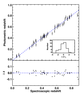
Figure 2.— $\it{Top}$: Weighted mean photometric redshift $z_{\mathrm{comb}}$ versus  spectroscopic redshift using the same sub-sample as in Figure 1. $\it{Bottom}$: the distribution of the redshift errors. The RMS scatter in $\Delta z/(1+z_{\mathrm{spec}})$=0.017. $\it{Inset}$: histogram of the normalized redshift error distribution, which is roughly Gaussian with RMS $\simeq 1$.

3.1.3 Spitzer Photometric Redshifts

For clusters where we do not have deep enough optical data to estimate a redshift but that do have Spitzer coverage, we use the algorithm used in Method 1 to measure the redshifts using Spitzer-only colors in the same manner as we do with optical data. Overdensities of red galaxies in clusters have been identified using Spitzer-only color selection at high redshift, where the IRAC bands are probing the peak of the stellar emission (Stern et al., 2005; Papovich, 2008), rather than bracketing the 4000Å break. Note that the concerns about the impact of recent star formation or AGN activity on photometric redshift estimates are not as serious in the IRAC bands as in the optical bands, because the portion of the spectrum probed is less sensitive to these potential sources of contamination. In our sample, the comparison of Spitzer-only redshifts with spectroscopically derived redshifts shows good performance, indicating that the assumption of a well-developed red-sequence appears to hold out to $z\gtrsim 1$ (e.g., Bower et al., 1992; Eisenhardt et al., 2008; Muzzin et al., 2009). Note that the possibility of the cluster being at lower redshift is already ruled out from the available optical data for these candidates.

Figure 3 shows the performance of the Spitzer-only redshifts in eight clusters where spectroscopic redshifts are available. Although the accuracy in $z_{\mathrm{phot}}$ is lower ($\Delta z/(1+z)\approx 0.049$) than those derived from optical-only or optical-IRAC colors, the performance is reliable. We flag these cases in the final table to make note of this difference in method. The larger uncertainties of Spitzer–only derived redshifts are possibly due to the broad width of IRAC filters and the fact that AGN emission or vigorous star formation can shift the location of the 1.6$\mu$m bump.

Figure 3.— Photometric redshift vs. $z_{\mathrm{spec}}$ for clusters where only the Spitzer IRAC 3.6$\mu$m-4.5$\mu$m colors are used. In all cases where we present Spitzer photo-z’s, we have optical data to rule out the presence of a low-redshift cluster.

3.1.4 Redshift Limits

In most cases there is an obvious, rich overdensity of red cluster galaxies in our follow-up imaging, from which it is straightforward to confirm the galaxy cluster giving rise to the SZ signal and to estimate the cluster redshift. For unconfirmed candidates, it is not possible to say with absolute certainty that no optical/NIR counterpart exists; with real, finite-depth optical and NIR data, the possibility always exists that the cluster is distant enough that no counterpart would have been detected at the achieved optical/NIR depth. Assigning a relative probability to these two interpretations of an optical/NIR non-detection (i.e., a false detection in the SZ data or a higher-redshift cluster than the optical/NIR observations could detect) is especially important for interpreting the SZ cluster sample cosmologically. To this end, we calculate a lower redshift limit for every SZ-selected candidate for which no counterpart has been found. Because the optical/NIR follow-up data is not homogeneous, we do this separately for each unconfirmed candidate.

To estimate the depth of the optical/NIR coadded images, we utilize a Monte-Carlo based technique described in Ashby et al. (2009). In brief, we perform photometry of the sky in various apertures at 1500 random positions in each image. To measure the sky noise, we then fit a Gaussian function to the resulting flux distribution (excluding the bright tail which is biased by real sources in the image). Taking the measured sky noise from 3″-diameter apertures, we add a PSF-dependent aperture correction. A redshift limit is derived for each filter by matching a 0.4$L^{*}$ red-sequence galaxy from the BC03 model to the measured 10$\sigma$ magnitude limit. We use the redshift limit from the second deepest filter with regards to 0.4$L^{*}$ red-sequence objects, as we require a minimum of two filters to measure a redshift. These redshift limits are compared to limits derived by comparing observed number counts of galaxies as a function of magnitude to distributions derived from much deeper data (Zenteno et al., 2011). We find the two independent redshift limit estimations are in good agreement.

For cluster candidates with Spitzer/IRAC observations, the redshift estimation is not limited by the depth of the optical data, and we use the IRAC data to calculate a lower redshift limit for these candidates. The IRAC data are highly uniform, with depth sufficient to extract robust photometry down to $0.1L^{*}$ out to a redshift of $z=1.5$. In principle, $\sim 0.5L^{*}$ photometry should be sufficient for redshift estimation; however, we adopt $z=1.5$ as a conservative lower redshift limit for any unconfirmed candidates with IRAC data.

3.2. NIR Overdensity Estimates for Unconfirmed Candidates

For cluster candidates for which we are unable to estimate a redshift, we can in principle go beyond a simple binary statement of “confirmed/unconfirmed” using NIR data. Even if there is not a sufficient number of galaxies in the NIR data to estimate a red sequence, there is information in the simple overdensity of objects (identified in a single NIR band) within a certain radius of an SPT candidate, and we can use this information to estimate the probability of that candidate being a real, massive cluster. We can then use this estimate to sharpen our estimate of the purity of the SPT-selected cluster sample. We calculate the single-band NIR overdensity for all unconfirmed candidates using WISE data, and we compare that value to the same statistic estimated on blank-field data. We perform the same procedure using Spitzer/IRAC and NEWFIRM data for unconfirmed candidates that were targeted with those instruments. For comparison, we also calculate the same set of statistics for each confirmed cluster above $z=0.7$.

We estimate the galaxy overdensity within a $1\ \mathrm{arcmin}^{2}$ aperture. To increase the signal-to-noise of the estimator, we assume an angular profile shape for the cluster galaxy distribution and fit the observed distribution to this shape. The assumed galaxy density profile is a projected $\beta$ model with $\beta=1$ (the same profile assumed for the SZ signal in the matched-filter cluster detection algorithm in R12). We have tried using a projected NFW profile as well, and the results do not change in any significant way (due to the relatively low signal-to-noise in the NIR data). The central amplitude, background amplitude, scale radius, and center position (with respect to the center of the SZ signal in SPT data) are free parameters in the fit. The number of galaxies above background within $1\ \mathrm{arcmin}^{2}$—which we will call $\Sigma_{1^{\prime}}$—is then calculated from the best-fit profile. The same procedure is repeated on fields not expected to contain massive galaxy clusters, and the value of $\Sigma_{1^{\prime}}$ for every SPT candidate is compared to the distribution of $\Sigma_{1^{\prime}}$ values in the blank fields. The key statistic is the fraction of blank fields that had a $\Sigma_{1^{\prime}}$ value larger than a given SPT candidate, and that value is recorded as $P_{\mathrm{blank}}$ in Table A for every high-redshift ($z\geq 0.7$) or unconfirmed candidate. This technique, including using the blank-field statistic as the primary result, is similar to the analysis of WISE data in the direction of unconfirmed Planck Early SZ clusters in Sayers et al. (2012), although that analysis used raw galaxy counts within an aperture rather than profile fitting.

The model fitting is performed using a simplex-based $\chi^{2}$ minimization, with any parameter priors enforced by adding a $\chi^{2}$ penalty. The positional offset $\chi^{2}$ penalty is $\Delta\chi^{2}=(\Delta\theta/\sigma_{\Delta\theta})^{2}$, where $\sigma_{\Delta\theta}$ is chosen to be 0.25′, based on the SZ/BCG offset distribution in Figure 7 and the value of $r_{200}$ for a typical-mass SPT cluster at high redshift. A prior is enforced on the scale radius from below and above by adding $\chi^{2}$ penalties of $(\theta_{s}/\theta_{s,\mathrm{max}})^{2}$ and $(\theta_{s,\mathrm{min}}/\theta_{s})^{2}$, where $\theta_{s,\mathrm{max}}$ is chosen to be 0.75′based on the $\theta_{s}$ distribution in known high-redshift SPT clusters with NIR data, and $\theta_{s,\mathrm{min}}$ is chosen to be 0.125′to prevent the fitter from latching onto small-scale noise peaks.

For Spitzer/IRAC and WISE, the fit is performed on the 3.6$\mu$m and the 3.4$\mu$m data, respectively; for NEWFIRM, the fit is performed on the $K_{s}$-band data. For both Spitzer/IRAC and NEWFIRM, a single magnitude threshold is used for every candidate; this threshold is determined by maximizing the signal-to-noise on the $\Sigma_{1^{\prime}}$ estimator on known clusters while staying safely away from the magnitude limit of the shallowest observations. The Spitzer/IRAC data is very uniform, and the 3.6$\mu$m magnitude threshold chosen is 18.5 (Vega). The NEWFIRM $K_{s}$-band data is less uniform, but a magnitude threshold of $18$ (Vega) is safe for all observations. For these instruments (IRAC and NEWFIRM), the blank fields on which the fit is performed come from the Spitzer Deep Wide-Field Survey (SDWFS) region (Ashby et al., 2009), which corresponds to the Bootes field of the NOAO Deep Wide-Field Survey (NDWFS; Jannuzi & Dey, 1999). The depth of the SDWFS/NDWFS observations for both instruments (19.8 in Vega for Spitzer/IRAC 3.6$\mu$m and 19.5 in Vega for NEWFIRM $K_{s}$) is more than sufficient for our chosen magnitude thresholds.

For WISE, in which the non-uniform sky coverage results in significant variation in magnitude limits, we perform the blank-field fit on data in the immediate area of the cluster (within a $\sim 20^{\prime}$ radius). Under the assumption that the WISE magnitude limit does not vary over this small an angular scale, we use all detected galaxies brighter than 18th magnitude (Vega) in both the cluster and blank-field fits.

3.3. Identifying rBCGs in SPT Clusters

An rBCG in this work is defined as the brightest galaxy among the red-sequence galaxies for each cluster. We employ the terminology rBCGs, rather than BCGs, to allow for the rare possibility of an even brighter galaxy with significant amounts of ongoing star formation, because the selection is restricted by galaxy colors along the cluster red sequence. We visually inspect pseudo-color images built with the appropriate filter combinations (given the cluster redshift) around the SZ candidate position. We search a region corresponding to the projected cluster virial region, defined by $\theta_{200}$, given the mass estimate from the observed cluster SPT significance $\xi$ and photometric redshift $z_{\mathrm{phot}}$.

There are 12 clusters out of the 158 with measured photometric redshifts (excluding the candidates with redshift limits) that are excluded from the rBCG selections. Eight of those are excluded due to contamination by a bright star that obscures more than one third of the area of the 3$\sigma$ SPT positional uncertainty region. Another cluster is excluded due to a bleed trail making the rBCG selection ambiguous, and three other clusters are excluded due to a high density in the galaxy population that, given the delivered image quality, makes it impossible to select the rBCG.

4. Results

The complete list of 224 SPT cluster candidates with SZ detection significance $\xi\geq 4.5$ appears in Table A. The table includes SZ cluster candidate positions on the sky [RA Dec], SZ detection significance [$\xi$], and spectroscopic redshift [$z_{\mathrm{spec}}$] when available. For confirmed clusters, the table includes photometric redshift and uncertainty [$z_{\mathrm{comb}}$$\pm$$\sigma_{z_{\mathrm{comb}}}$], estimated as described in §3.1. Unconfirmed candidates are assigned redshift lower limits, estimated as described in §3.1.4.

We also report a redshift quality flag for each $z_{\mathrm{phot}}$ in Table A. For most of the confirmed clusters with reliable photometric redshift measurements, we set Flag = 1. There is one cluster (SPT-CL J2146-4846) for which the three individual photometric redshifts are not statistically consistent ($\gtrsim 3\sigma$ outliers) for which we set Flag = 2. We still report the combined redshift for that cluster as in other secure systems. We have 6 cases where we only use Swope + Method 1, and 25 cases where we only use Spitzer + Method 1 for redshift estimation, both cases marked with Flag = 3. We note that the photometric redshift bias correction for two clusters (SPT-CL J0333-5842 and SPT-CL J0456-6141) is at a higher level than the typical bias correction on other clusters (see 3.1.1 for more detail on the bias correction. There are 2 cases (SPT-CL J0556-5403 and SPT-CL J0430-6251) where we quote only a Method 1 redshift even for MOSAIC or IMACS data, marked with Flag = 4. In the coadded optical images for SPT-CL J0556-5403, we identify an overdensity of faint red galaxies at the location of the SPT candidate. This optical data is too shallow, however, to allow for secure redshift estimation, but we are able to measure a redshift by combining this data with NEWFIRM imaging. This cluster is the only candidate where we rely on photometric redshift from $i$-$K_{s}$. SPT-CL J0430-6251 is in a field very crowded with large scale structure, making redshift estimation difficult.

In the Appendix, we discuss certain individually notable candidates—such as associations with known clusters that appear to be random superpositions and candidates with no optical/NIR confirmation but strong evidence from the NIR overdensity statistic.

Figure 4.— Redshift histogram of 158 confirmed clusters, in bins of $\Delta z=0.1$. Note that about 18% of the total sample comes from $z\geq 0.8$.

4.1. Redshift Distribution

The redshift distribution for the 158 confirmed clusters is shown in Figure 4. The median redshift is $z=0.57$, with 28 systems ($\sim$18% of the sample) lying at $z>0.8$. The cluster with the highest photometric redshift is SPT-CL J2040-4451 at $z=1.35\pm 0.07$ (estimated using Spitzer/IRAC data) and the highest-redshift spectroscopically confirmed cluster is SPT-CL J0205-5829 at $z=1.32$. (This cluster is discussed in detail in Stalder et al. 2012.)

The high fraction of SPT clusters at $z>0.8$ is a consequence of the redshift independence of the SZ surface brightness and the arcminute angular resolution of the SPT, which is well-matched to the angular size of high-$z$ clusters. X-ray surveys, in contrast, are highly efficient at finding nearby clusters, but the mass limit of an X-ray survey will increase with redshift due to cosmological dimming. ROSAT cluster surveys lack the sensitivity to push to these high redshifts except in the deepest archival exposures. XMM–Newton archival surveys (e.g., Lloyd-Davies et al., 2011; Fassbender et al., 2011) and coordinated surveys of contiguous regions (e.g., Pacaud et al., 2007; Šuhada et al., 2012) have sufficient sensitivity to detect systems like those found by SPT, but the solid angle surveyed is currently smaller. For example, the Fassbender et al. (2011) survey for high redshift clusters will eventually cover approximately 80 deg², whereas the mean sky density of the SPT high-redshift and high-mass systems is around one every 25 deg². Therefore, one would have expected the Fassbender et al. (2011) XDCP survey to have found around three clusters of comparable mass to the SPT clusters, which is in fact consistent with their findings. The vast majority of the high redshift X-ray-selected sample available today is of significantly lower mass than SPT selected samples, simply because the X-ray surveys do not yet cover adequate solid angle to find these rare, high mass systems.

Clusters samples built from NIR galaxy catalogs have an even higher fraction of high-redshift systems than SZ-selected samples—for example, in the IRAC Shallow Cluster Survey (ISCS; Eisenhardt et al., 2008) a sample of 335 clusters has been identified out to $z\sim 2$, a third of which are at $z>1$. However, the typical ISCS cluster mass is $\sim 10^{14}$ M_⊙ (Brodwin et al., 2007), significantly lower than the minimum mass of the SPT high-redshift sample. As with the X-ray selected samples, the Spitzer sample includes some massive clusters, including the recently discovered IDCS J1426.5+3508 at $z=1.75$, which was subsequently also detected in the SZ (Stanford et al., 2012; Brodwin et al., 2012). However, the Spitzer surveys to date do not cover the required solid angle to find these massive systems in the numbers being discovered by SPT.

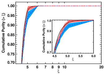
Figure 5.— Cumulative purity estimates derived from the optical/NIR followup compared to simulated purity predictions (solid black line). The inset plot is zoomed-in to the $\xi$ range between 4.5 and 6.0 and binned more finely. The purity is calculated from the follow-up confirmation rate: 1) (dashed blue) assuming all clusters without a clear optical or NIR counterpart are false SZ detections (i.e., 100% optical completeness) and all optical confirmations are robust (100% optical purity); and 2) (dash-dot-dot red) assuming, as justified in the text, 97% optical completeness and 96% optical purity but taking into account clusters confirmed through other means such as X-ray observations. 1$\sigma$ uncertainties in the purity estimates from follow-up are shown with shaded blue or red regions (see Section 4.2).

4.2. Purity of the SPT Cluster Candidates

For a cluster sample to be useful for cosmological purposes, it is important to know the purity of the sample, defined as

$$f_{\mathrm{pure}}=\frac{N_{\mathrm{real}}}{N_{\mathrm{tot}}}=1-\frac{N_{\mathrm{false}}}{N_{\mathrm{tot}}},$$ (3)

where $N_{\mathrm{tot}}$ is the total number of cluster candidates, $N_{\mathrm{real}}$ is the number of candidates corresponding to real clusters, and $N_{\mathrm{false}}$ is the number of false detections. For an SZ-selected cluster sample with reasonably deep and complete optical/NIR follow-up, a first-order estimate of $N_{\mathrm{real}}$ is simply the number of candidates with successfully estimated redshifts. In Figure 5, we show two estimations of purity for the 720 deg² SPT-SZ sample; the first in blue, assuming that all cluster candidates with no redshift measurements are noise fluctuations, and the other in red, taking into account incompleteness of our follow-up data. The blue/red shaded regions in the figure correspond to the 1$\sigma$ uncertainties on the purity, estimated from Poisson noise on $N_{\mathrm{false}}$ for the blue region and as described below for the red region. We also show the expected purity, estimated from the total number of candidates in the sample presented in this work combined with the false detection rate from the simulations used to test the SZ cluster finder (R12 Figure 1).

The possibility of real clusters beyond the redshift reach of our optical/NIR redshift estimation techniques makes the blue line in Figure 5 a lower limit to the true purity of the sample. As discussed in §3.2, we use single-band NIR data to estimate the probability that each unconfirmed candidate is a “blank field”, i.e., a field with typical or lower-than-typical NIR galaxy density. Candidates with no optical/NIR confirmation but with a low blank field probability $P_{\mathrm{blank}}$, are potential high-redshift systems that merit further follow-up study. These systems can also give an indication of how much we underestimate our sample purity when we assume any optical/NIR non-confirmation is a spurious SPT detection. By definition, a low $P_{\mathrm{blank}}$ implies some NIR overdensity towards the SPT detection, but perhaps not large enough to be an SPT-detectable cluster. We can roughly calibrate the $P_{\mathrm{blank}}$ values to SPT detectability by investigating the results of the NIR overdensity estimator on solidly confirmed, high-redshift SPT clusters. There are 19 clusters with spectroscopic redshifts above $z=0.7$, and the average Spitzer/IRAC $P_{\mathrm{blank}}$ value for these clusters is $0.04$, while the average WISE $P_{\mathrm{blank}}$ value is $0.05$. Only three of these clusters have NEWFIRM data, and the average NEWFIRM $P_{\mathrm{blank}}$ value is $0.07$. Only one cluster in this high-$z$ spectroscopic sample has an IRAC $P_{\mathrm{blank}}>0.1$, while three have WISE $P_{\mathrm{blank}}>0.1$. So a rough threshold for SPT-type clusters appears to be $P_{\mathrm{blank}}\leq 0.1$. We have nine unconfirmed cluster candidates that meet this criterion in at least one of the NIR catalogs, including five that are at $P_{\mathrm{blank}}\leq 0.05$. If we assumed all of the $P_{\mathrm{blank}}\leq 0.05$ clusters were real, it would imply that the completeness of the optical/NIR redshift estimation was $\sim 97\%$, i.e., we have 163 real clusters of which we were able to estimate redshifts for 158.

Conversely, the possibility of false associations of spurious SZ detections with optical/NIR overdensities would act in the other direction. Tests of one of the red-sequence methods on blank-field data produced a significant red-sequence detection on approximately $4\%$ of fields without SPT detected clusters. Assuming that the cross-checks with other methods would remove some of these, we can take this as an upper limit to this effect.

We therefore provide a second estimate of purity from the optical/NIR confirmation rate, taking into account the possibility of real clusters for which we were unable to successfully estimate a redshift (redshift completeness $<100\%$) and spurious optical/NIR associations with SPT noise peaks (redshift purity $<100\%$). From the above arguments, we assume 97% for redshift completeness and 96% for redshift purity. For each value of SPT significance $\xi$, we use binomial statistics to ask how often a sample of a given purity with total candidates $N(>\xi)$ would produce the observed number of successful optical/NIR redshift estimates $N_{\mathrm{conf}}(>\xi)$, given the redshift completeness and false rate. An extra constraint is added to this calculation based on data independent of the optical/NIR imaging that confirms many of the SPT candidates as real, massive galaxy clusters. Specifically, we assume an SPT candidate is a real, massive cluster independent of the optical/NIR imaging data (and remove the possibility of that candidate being a false optical/NIR confirmation of an SPT noise peak) if: 1) it is associated with a ROSAT Bright Source Catalog source; 2) we have obtained X-ray data in which we can confirm a strong, extended source; or 3) we have obtained spectroscopic data and measured a velocity dispersion for that system. The red solid line and shaded region in Figure 5 show the maximum-likelihood value and $68\%$ limits for the true purity of the SPT sample under these assumptions.

The purity measured in this work is in good agreement with the model for the SPT sample purity. In particular, all clusters with $\xi>6$ have identified optical counterparts with photometric redshift estimates. This is consistent with the expectation of the model and a demonstration that the SPT selected galaxy cluster sample is effectively uncontaminated at $\xi>6$. With decreasing significance, the number of noise fluctuations in the SPT maps increases compared to the number of real clusters on the sky, and the purity decreases. The cumulative purity of the sample is $\sim$70% above $\xi=4.5$ and reaches $\sim$100% above $\xi=5.9$. Of course, if one requires optical confirmation in addition to the SPT detection, then the sample is effectively 100% pure over the full sample at $\xi>4.5$.

=We note that there is no significant difference in false detection rate (based on optical confirmation alone) between cluster candidates selected with 150 GHz data alone and those detected with the multiband strategy (see §2.1 for details). Roughly 1/4 of the survey area was searched for clusters using 150 GHz data only, and in that area we have 12 unconfirmed candidates, including one above $\xi=5$; in the 3/4 of the area selected using multiband data, we have 54 unconfirmed candidates, including five above $\xi=5$. These totals are consistent within $1\sigma$ Poisson uncertainties.

The high purity of the SPT selected cluster sample is comparable to the purity obtained in previous X-ray cluster surveys (i.e. Vikhlinin et al., 1998; Mantz et al., 2008; Vikhlinin et al., 2009), indicating that these intracluster medium based selection techniques, when coupled with optical follow-up, provide a reliable way to select clean samples of clusters for cosmological analysis.

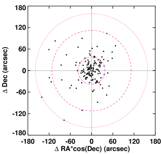
Figure 6.— rBCG positions are plotted as offsets from SPT candidate positions for 146 systems with clearly defined rBCGs. The magenta concentric circles enclose 68% (dash-dot line), 95% (dashed line) and 99% (dotted line) of the whole rBCG sample and have radii of 38.0″, 112.1″and 158.6″.

4.3. rBCG Offsets in SPT Clusters

The position of the rBCG in galaxy clusters is a property of interest for both astrophysical and cosmological cluster studies, as it is a possible indication of a cluster’s dynamical state. In relaxed clusters, it is expected that dynamical friction will tend to drive the most massive galaxies to the bottom of the cluster potential well, which would coincide with the centroid of the X–ray and SZ signatures. On the other hand, in cases of merging systems one would expect two different rBCGs, and one or both could appear well-separated from the X-ray or SZ centroid. Several studies have shown a tight correlation between the X-ray centroid and the rBCG position (Lin & Mohr, 2004; Haarsma et al., 2010; Mann & Ebeling, 2012; Stott et al., 2012), although Fassbender et al. (2011) provide evidence that at high redshift the BCG distribution is less centrally peaked. Here we examine the rBCG positions with respect to the centroid of the SZ signal in the SPT cluster sample.

The position of each rBCG is listed in Table A, and the offsets from the SZ centroids in arcsec are plotted in Figure 6. The rings correspond to different fractions of the full population of clusters: 68%, 95%, and 99%. These rings have radii of 38.0″, 112.1″and 158.6″, respectively. The rBCG population is centrally concentrated with the bulk of the SPT selected clusters having rBCGs lying within about 1^′ of the candidate position.

Given the broad redshift range of the cluster sample, the rBCG distribution in cluster coordinates $r/r_{200}$ is more physically interesting. We use the cluster redshifts from this work and the SZ-derived masses from R12 to calculate $r_{200}$ for each cluster. The red line in Figure 7 is the cumulative distribution of the rBCGs as a function of $r/r_{200}$. In this distribution, 68% of the rBCGs lies within 0.17$r_{200}$, 95% within 0.43$r_{200}$ and 99% within 0.70$r_{200}$.

We check for any effects of mm-wave selection and redshift estimation on the rBCG offset distribution by splitting the sample three ways: 1) clusters selected using 150 GHz data only vs. clusters selected using multiband data; 2) clusters with spectroscopic redshifts vs. clusters with photometric redshifts only; 3) clusters with secure photometric redshifts (Flag = 1) vs. clusters with flagged redshifts (Flag $>$ 1, see §4 for details). We see no evidence that the rBCG offsets (in units of $r_{200}$) in these subsamples are statistically different. A Kolmogorov-Smirnov (KS) test results in probabilities of $84\%$, $39\%$, and $34\%$ that these respective subsamples are drawn from the same underlying distribution.

We investigate the importance of the SPT candidate positional uncertainty by modeling the expected radial distribution in the case where all rBCGs are located exactly at the cluster center. The $1\sigma$ SPT positional uncertainty for a cluster with a pressure profile given by a spherical $\beta$ model with $\beta=1$ and scale size $\theta_{c}$, detected by SPT at significance $\xi$, is given by

$$\Delta\theta=\sqrt{(\theta_{\mathrm{beam}}^{2}+(k\theta_{c})^{2})}/\xi,$$ (4)

where $\theta_{\mathrm{beam}}$ is the beam FWHM, and $k$ is a factor of order unity (see Story et al. 2011 for more details). With this information, we estimate the expected cumulative distribution of the observed rBCG offsets, assuming a Gaussian with the appropriate width for each cluster; this is equivalent to assuming the underlying rBCG distribution is a delta function centered at zero offset with respect to the true cluster SZ centroid. Results are shown as the blue dotted curve in Figure 7. It is clear that the observed distribution of rBCG offsets is broader than that expected if all rBCGs were located exactly at the cluster center. We conduct a Kolmogorov-Smirnov (KS) test to address the similarity of the two distributions. The hypothesis that the two distributions are drawn from the same parent distribution has a probability of 0.09%, suggesting that the observed rBCG offset distribution cannot be easily explained by the SPT positional uncertainties alone.

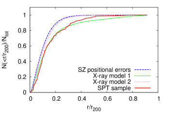
Figure 7.— Normalized cumulative distribution of rBCG offsets from SPT candidate positions as a function of $r/r_{200}$ for the SPT cluster sample (red solid line), the expected distribution given SPT positional uncertainties if all rBCGs were at exactly the center of the true SZ centroid (blue dash-dot line), and the expected distribution given SPT positional uncertainties if the underlying distribution of offsets matched those of two different X-ray selected cluster samples (green dashed line; Lin & Mohr, 2004) and (magenta dotted line; Mann & Ebeling, 2012). The KS probability that the observed rBCG distribution and the SPT positional error distribution are drawn from the same parent distribution is 0.09%, but the observed distribution is statistically consistent with the distribution from the X-ray-selected sample convolved with the SPT positional uncertainty distribution. There is no evidence in the rBCG offset distribution that SPT-selected clusters are more merger-rich than X-ray-selected clusters.

Because the SPT candidate positional uncertainties $\Delta\theta$ are roughly the same, one can expect that our ability to measure the underlying rBCG distribution will weaken as we push to higher redshift where the cluster virial regions subtend smaller angles on the sky. We test this by dividing the sample into four redshift bins with similar numbers of members. The KS tests confirm our expectations; using redshift bins of 0.0-0.40, 0.40-0.54, 0.54-0.73 and $z>0.73$ we find the probability that the observed and positional error distributions are drawn from the same parent distribution is 0.11%, 0.008%, 1.97% and 43.4%, respectively. Thus, with the current cluster sample, we cannot detect any extent in the rBCG distribution beyond a redshift $z\sim 0.7$. If we assume the underlying rBCG offset distribution is Gaussian, the KS test shows a maximum probability of 5.3% for a Gaussian distributed width of 0.074$r_{200}$ with the probability of consistency dropping below 0.1% for $\sigma>0.08r_{200}$. Therefore, while the Gaussian is not a particularly good fit, the measured distribution strongly favors $\sigma<0.08r_{200}$.

We test whether our SZ-selected cluster sample exhibits similar rBCG offsets to those seen in previous X-ray studies. To do this, we adopt the previously published BCG offset distribution from the X-ray studies as the underlying BCG offset distribution for our sample and then convolve this distribution with the SPT candidate positional uncertainties. If rBCGs in SZ-selected clusters are no different from those in these previously studied samples, then we would expect the KS test probability of consistency to be high. We explore two samples: X-ray model 1 (Lin & Mohr 2004; green dashed line in Figure 7) and X-ray model 2 (Mann & Ebeling 2012; magenta dotted line in Figure 7). The probability of consistency between the SPT sample and X-ray model 1 is 41%, and the probability of consistency between the SPT sample and X-ray model 2 is 0.46%. We also examine another X-ray sample (Stott et al., 2012) which produces a very similar result with our X-ray model 2 with the probability of consistency of 0.55%.

It appears likely that the differences between the two previously published X-ray samples can be explained in terms of differences in the BCG selection. The measured rBCG offset distribution presented in this work agrees with the Lin & Mohr (2004) sample, in which the BCGs were defined as the brightest $K$-band galaxy projected within the virial radius $\theta_{200}$ with spectroscopic redshift consistent with the cluster redshift. This BCG selection is very similar to the SPT rBCG selection, with the main difference being that we do not have spectroscopic redshifts for all rBCG candidates in the SPT sample. The agreement between the SZ- and X-ray-selected samples in this case suggests that there are no strong differences between the merger fractions in these two cluster samples.

The Mann & Ebeling (2012) BCG sample, in contrast, was assembled using bluer optical bands, which are more sensitive to the star formation history. In addition, in cases where a second concentration of galaxies was found within the projected virial region, the central galaxy of the galaxy concentration coincident with the X-ray emission peak was chosen as the BCG, regardless of whether it was brighter or not (Mann, private communication). This selection criteria would make it difficult to identify significantly offset BCGs, which would be more likely to be present in merging systems. Similarly, the Stott et al. (2012) BCG sample was assembled using $i$-band data and a prior on the offset that excludes any offset greater than 500 kpc. Such a prior would also bias the measured distribution against large offsets due to ongoing merger activity.

The rBCG offset distribution measured in the SPT SZ-selected sample of clusters does not provide any compelling evidence that SZ-selected clusters differ in their merger rate as compared to X-ray-selected clusters. It will be possible to test this more precisely once we have the more accurate X-ray cluster centers with consistent rBCG selections. Currently, the X-ray properties of only 15 SPT SZ-selected clusters have been published (Andersson et al., 2011; Benson et al., 2011); however, over 100 additional SPT selected clusters have been approved for observation in on-going programs with Chandra and XMM-Newton. With those data in hand we will be able to measure the rBCG offset distribution over the full redshift range of SPT clusters, allowing us to probe for evolution in the merger rates with redshift.

5. Conclusions

The SPT-SZ survey has produced an approximately mass-limited, redshift-independent sample of clusters. Approximately 80% of these clusters are newly discovered systems; the SPT survey has significantly increased the number of clusters discovered through the SZ effect and the number of massive clusters detected at high redshift. In this paper, we present optical/NIR properties of 224 galaxy cluster candidates selected from 720 deg² of the SPT survey that was completed in 2008 and 2009. The results presented here constitute the subset of the survey in which the optical/NIR follow-up is essentially complete.

With a dedicated pointed follow-up campaign using ground- and space-based optical and NIR telescopes, we confirm 158 out of 224 SPT cluster candidates and measure their photometric redshifts. We show that 18% of the optically confirmed sample lies at $z>0.8$, the median redshift is $z=0.57$, and the highest redshift cluster is at $z=1.35\pm 0.07$. We have undertaken a cross-comparison among three different cluster redshift estimators to maximize the precision in the presented photometric redshifts. For each cluster, we combine the redshift estimates from the three methods, accounting for the covariance among the methods. Using 57 clusters with spectroscopic redshifts, we calibrate the photometric redshifts and uncertainties and demonstrate that our combining procedure provides a characteristic final cluster redshift accuracy of $\Delta z/(1+z)=0.017$.

For the 66 candidates without photometric redshift measurements, we calculate lower redshift limits. These limits are set by the depth of the optical/NIR imaging and the band combinations used. For nine of these candidates there is evidence from NIR data that the cluster is a high redshift system, and that we simply need deeper NIR data to measure a photometric redshift.

Under the assumption that all 66 candidates without photometric redshift measurements are noise fluctuations, we estimate the purity of the SPT selected cluster sample as a function of the SPT detection significance $\xi$. Results are in good agreement with expectations for sample purity, with no single unconfirmed system above $\xi=6$, $>95\%$ purity above $\xi=5$, and $\sim 70\%$ purity for $\xi>4.5$. By requiring an optical/NIR counterpart for each SPT candidate, the purity in the final cluster sample approaches 100% over the full $\xi>4.5$ sample. The purity of the SPT cluster sample simplifies its cosmological interpretation.

Next, we examine the measured rBCG offset from the SZ candidate positions to explore whether SZ-selected clusters exhibit similar levels of ongoing merging as X-ray selected samples. We show that the characteristic offset between the rBCG and the candidate position is $\sim$0.5^′. We examine the radial distribution of rBCG offsets as a function of scaled cluster radius $r/r_{200}$ and show that a model where we include scatter due to SPT positional uncertainties assuming all BCGs are at cluster centers has only a 0.09% chance of consistency with the observed distribution. That is, the observed distribution is broader than would be expected from SPT positional uncertainties alone. If we assume the rBCG offset distribution is Gaussian, the observations rule out a Gaussian width of $\sigma>0.08r_{200}$, however, even with smaller width a Gaussian distribution is only marginally consistent with the data. When comparing the SPT rBCG distribution with a X-ray selected cluster sample with a similar rBCG selection criteria (Lin & Mohr, 2004), the SPT and X-ray selected rBCG distributions are similar, suggesting that their merger rates are also similar. Comparisons to other X-ray selected samples are complicated by differences in rBCG selection criteria. For example, comparing to Mann & Ebeling (2012), which selects BCGs using bluer optical bands, we find a significantly less consistent rBCG distribution compared to SPT. We conclude that SZ and X-ray selected cluster samples show consistent rBCG distributions, and note that BCG selection criteria can have a significant effect in such comparisons.

With the full 2500 $\mathrm{deg}^{2}$ SZ survey completed in 2011, we are now working to complete the confirmations and redshift measurements of the full cluster candidate sample. Scaling from this 720 deg² sample with effectively complete optical follow-up, we estimate that the full survey will produce $\sim$500 confirmed clusters, with approximately 100 of them at $z>0.8$. This sample of clusters will enable an important next step in cluster cosmological studies as well as the first detailed glimpse of the high redshift tail of young, massive clusters.

Appendix A Notable clusters

SPT-CL J0337-6207

This candidate is optically unconfirmed but has small NIR blank-field probability in at least one data set ($P_{\mathrm{blank}}=0.5\%$ in WISE data—also, $P_{\mathrm{blank}}=18.2\%$ in NEWFIRM data—see §3.2 for details).

SPT-CL J0428-6049

This candidate is optically unconfirmed but has a high SPT significance ($\xi=5.1$) and small NIR blank-field probability in at least one data set ($P_{\mathrm{blank}}=0.5\%$ in WISE data, see §3.2 for details). Though $P_{\mathrm{blank}}=69.0\%$ in NEWFIRM data, there is clear visual evidence of a NIR overdensity in the NEWFIRM images, but at $\sim 40\arcsec$ from the SPT position. Such a large offset is heavily disfavored by the fitting procedure, such that the model that minimizes the overall $\chi^{2}$ for the NEWFIRM data is effectively a blank field. The position of the WISE overdensity is consistent with the SPT position.

SPT-CL J0458-5741

This cluster is listed as optically unconfirmed, but it is also listed in Table 2 of R12 as coincident with the low-redshift cluster ACO 3298 (at a separation of $77\arcsec$). We see a clear red-sequence overdensity in our Magellan/IMACS data at $z\simeq 0.2$, centered on the Abell cluster position. The best-fit SZ core radius for this candidate is $2.5\arcmin$, which implies an SPT positional uncertainty of $\sim 0.5\arcmin$, in which case a $77\arcsec$ offset is only a $\sim 2\sigma$ outlier. However, visual inspection of a lightly filtered SPT map shows that the SZ signal is coming from two distinct components, one of which corresponds to the Abell cluster position, and neither of which would have been significant enough to be included in the R12 catalog on its own. For this reason, we leave the $\theta_{c}=2.5\arcmin$ candidate, which blends the SZ signal from the two individual components, as unconfirmed.

SPT-CL J2002-5335

This candidate is optically unconfirmed but has small NIR blank-field probability in at least one data set ($P_{\mathrm{blank}}=7.5\%$ in WISE data—see §3.2 for details).

SPT-CL J2032-5627

This cluster is listed in Table 2 of R12 as coincident with the $z=0.06$ cluster ClG 2028.3-5637 / ACO 3685 (at a separation of $115\arcsec$ from the literature Abell cluster position) and as coincident with the $z=0.14$ cluster RXC J2032.1-5627 (at a separation of $87\arcsec$ from the reported REFLEX cluster position). However, from our Magellan/IMACS imaging data, we estimate a red-sequence redshift of $z=0.31\pm 0.02$, and, using the red-sequence measurements as a criterion for cluster member selection, we have obtained spectra for 32 cluster members using GISMO and have measured a robust spectroscopic redshift of $z_{\mathrm{spec}}=0.2840$. Examination of the REFLEX spectroscopic catalog (Guzzo et al., 2009) reveals that their spectroscopic observations yielded five galaxies near their reported redshift of $z_{\mathrm{spec}}=0.1380$ but also six galaxies within $2\%$ of the value we derive from our GISMO observations ($z_{\mathrm{spec}}=0.2840$). The value of $z_{\mathrm{spec}}=0.0608$ for ACO 3685 is from only one galaxy (and, while reported in Struble & Rood 1999, is originally from Fetisova 1981). We conclude that there are two clear optical overdensities at different redshifts along the line of sight to this SZ/X-ray system, and that the literature redshift of $z=0.0608$ for ACO 3685 is probably incorrect. Because of the redshift dependence of the SPT selection function (see, e.g., Vanderlinde et al. 2010), it is likely that the bulk of the SZ signal is coming from the higher-redshift cluster. We have obtained XMM–Newton data on this system, and the X-ray and SZ signals have very similar morphology, indicating that the X-ray signal is also predominantly associated with the higher-redshift system. This makes it likely that the $z=0.2840$ system is a massive cluster and that the $z=0.1380$ system is a low-mass interloper, possibly the cluster originally identified as ClG 2028.3-5637 / ACO 3685. SPT-CL J2032-5627 is discussed further—including weak lensing data from Magellan/Megacam—in High et al. (2012).

SPT-CL J2035-5614

This candidate is optically unconfirmed but has small NIR blank-field probability in at least one data set ($P_{\mathrm{blank}}=0.1\%$ in WISE data—see §3.2 for details).

SPT-CL J2039-5723

This candidate is optically unconfirmed but has a small SZ core radius ($0.5\arcmin$) and small NIR blank-field probability in at least one data set ($P_{\mathrm{blank}}=1.2\%$ in WISE data and $8.7\%$ in NEWFIRM data—see §3.2 for details).

SPT-CL J2121-5546

This candidate is optically unconfirmed but has small NIR blank-field probability in at least one data set ($P_{\mathrm{blank}}=0.9\%$ in WISE data–also, $P_{\mathrm{blank}}=11.5\%$ in NEWFIRM data—see §3.2 for details).

SPT-CL J2136-5535

This candidate is optically unconfirmed but has small NIR blank-field probability in at least one data set ($P_{\mathrm{blank}}=5.2\%$ in WISE data—see §3.2 for details).

SPT-CL J2152-4629

This candidate is optically unconfirmed but has a high SPT significance ($\xi=5.6$), a small SZ core radius ($0.25\arcmin$), and small NIR blank-field probability in at least one data set ($P_{\mathrm{blank}}=8.0\%$ in WISE data; also $P_{\mathrm{blank}}=10.6\%$ in Spitzer/IRAC data and $20.0\%$ in NEWFIRM data—see §3.2 for details). This is the only candidate with Spitzer/IRAC $P_{\mathrm{blank}}<20\%$ for which we were not able to estimate a redshift.

SPT-CL J2343-5556

This candidate is optically unconfirmed but has small NIR blank-field probability in at least one data set ($P_{\mathrm{blank}}=5.6\%$ in WISE data and $21.0\%$ in NEWFIRM data—see §3.2 for details).

Table 3All candidates above $\xi=4.5$ in 720 deg² of the SPT-SZ survey.

SPT ID	POSITION		$\xi$	$z_{\mathrm{spec}}$	$z_{\mathrm{comb}}$$\pm$ $\sigma_{z_{\mathrm{comb}}}$	Flag	NIR blank field probability $P_{\mathrm{blank}}$(%)			rBCG POSITION		Imaging Ref.
	RA (deg)	Dec (deg)			(or redshift lower limit)		NEWFIRM	Spitzer	WISE	RA (deg)	Dec (deg)
SPT-CLJ0000-5748	0.2496	-57.8066	5.48	0.702	0.68 $\pm$ 0.03	1	–	–	–	0.2503	-57.8093	1,2
SPT-CLJ0201-6051	30.3933	-60.8592	4.83	–	$>$ 1.0	–	61.3	–	100.0	–	–	1
SPT-CLJ0203-5651	30.8309	-56.8612	4.98	–	$>$ 1.0	–	28.1	–	56.5	–	–	1
SPT-CLJ0205-5829	31.4437	-58.4855	10.54	1.322	1.30 $\pm$ 0.07	3	8.0	2.0	1.8	31.4510	-58.4803	1
SPT-CLJ0205-6432	31.2786	-64.5461	6.02	0.744	0.75 $\pm$ 0.03	1	6.8	0.5	17.3	31.3244	-64.5583	1
SPT-CLJ0209-5452	32.3491	-54.8794	4.52	–	0.42 $\pm$ 0.03	1	–	–	–	32.3494	-54.8720	1
SPT-CLJ0211-5712	32.8232	-57.2157	4.77	–	$>$ 1.0	–	26.7	–	56.1	–	–	1
SPT-CLJ0216-5730	34.1363	-57.5100	4.72	–	$>$ 1.0	–	43.4	–	80.6	–	–	1,2
SPT-CLJ0216-6409	34.1723	-64.1562	5.54	–	0.64 $\pm$ 0.03	1	–	–	–	34.1599	-64.1599	1
SPT-CLJ0218-5826	34.6251	-58.4386	4.54	–	0.57 $\pm$ 0.03	1	–	–	–	34.6267	-58.4421	1,2
SPT-CLJ0221-6212	35.4382	-62.2044	4.71	–	$>$ 1.2	–	75.7	–	84.9	–	–	1
SPT-CLJ0230-6028	37.6410	-60.4694	5.88	–	0.74 $\pm$ 0.08	3	–	11.3	0.3	37.6354	-60.4628	3
SPT-CLJ0233-5819	38.2561	-58.3269	6.64	0.663	0.76 $\pm$ 0.07	3	4.2	0.0	–	38.2541	-58.3269	1
SPT-CLJ0234-5831	38.6790	-58.5217	14.65	0.415	0.42 $\pm$ 0.03	1	–	–	–	38.6762	-58.5236	1
SPT-CLJ0239-6148	39.9120	-61.8032	4.67	–	$>$ 1.1	–	44.2	–	38.0	–	–	1,2
SPT-CLJ0240-5946	40.1620	-59.7703	9.04	0.400	0.41 $\pm$ 0.03	1	–	–	–	40.1599	-59.7635	3
SPT-CLJ0240-5952	40.1982	-59.8785	4.65	–	0.62 $\pm$ 0.03	3	–	–	–	40.2048	-59.8732	5
SPT-CLJ0242-6039	40.6551	-60.6526	4.92	–	$>$ 1.5	–	–	51.5	64.9	–	–	2
SPT-CLJ0243-5930	40.8616	-59.5132	7.42	–	0.65 $\pm$ 0.03	1	–	–	–	40.8628	-59.5172	3
SPT-CLJ0249-5658	42.4068	-56.9764	5.44	–	0.23 $\pm$ 0.02	1	–	–	–	42.3918	-56.9870	1
SPT-CLJ0253-6046	43.4605	-60.7744	4.83	–	0.44 $\pm$ 0.02	1	–	–	–	43.4508	-60.7499	1
SPT-CLJ0254-5857	43.5729	-58.9526	14.42	0.438	0.43 $\pm$ 0.03	1	–	–	–	43.5365	-58.9718	3
SPT-CLJ0254-6051	43.6015	-60.8643	6.71	–	0.44 $\pm$ 0.02	1	–	–	–	43.5884	-60.8689	1
SPT-CLJ0256-5617	44.1009	-56.2973	7.54	–	0.63 $\pm$ 0.03	1	–	–	–	44.0880	-56.3031	3
SPT-CLJ0257-5732	44.3516	-57.5423	5.40	0.434	0.42 $\pm$ 0.02	1	–	–	–	44.3373	-57.5484	1
SPT-CLJ0257-5842	44.3924	-58.7117	5.38	–	0.42 $\pm$ 0.02	1	–	–	–	44.4374	-58.7045	1
SPT-CLJ0257-6050	44.3354	-60.8450	4.76	–	0.48 $\pm$ 0.03	1	–	–	–	44.3386	-60.8358	2
SPT-CLJ0258-5756	44.5563	-57.9438	4.50	–	$>$ 1.0	–	–	–	17.4	–	–	1,2
SPT-CLJ0300-6315	45.1430	-63.2643	4.88	–	$>$ 1.5	–	–	31.6	63.6	–	–	1
SPT-CLJ0301-6456	45.4780	-64.9470	4.94	–	0.65 $\pm$ 0.03	1	–	–	–	45.4809	-64.9492	1
SPT-CLJ0307-6226	46.8335	-62.4336	8.32	–	0.61 $\pm$ 0.03	1	–	–	–	46.8495	-62.4028	3
SPT-CLJ0311-6354	47.8283	-63.9083	7.33	–	0.30 $\pm$ 0.02	1	–	–	–	47.8229	-63.9157	1
SPT-CLJ0313-5645	48.2604	-56.7554	4.82	–	0.63 $\pm$ 0.03	1	–	–	–	48.2912	-56.7420	1
SPT-CLJ0316-6059	49.2179	-60.9849	4.59	–	$>$ 1.5	–	–	26.4	26.9	–	–	1
SPT-CLJ0317-5935	49.3208	-59.5856	5.91	0.469	0.47 $\pm$ 0.02	1	–	–	–	49.3160	-59.5915	1
SPT-CLJ0320-5800	50.0316	-58.0084	4.54	–	$>$ 1.0	–	–	–	38.1	–	–	1,2
SPT-CLJ0324-6236	51.0530	-62.6018	8.59	–	0.74 $\pm$ 0.03	1	–	0.3	0.0	51.0511	-62.5988	3
SPT-CLJ0328-5541	52.1663	-55.6975	7.08	0.084	0.10 $\pm$ 0.03	1	–	–	–	52.1496	-55.7124	1
SPT-CLJ0333-5842	53.3195	-58.7019	4.54	–	0.49 $\pm$ 0.04	3∗	–	–	–	53.3322	-58.7060	5
SPT-CLJ0337-6207	54.4720	-62.1176	4.88	–	$>$ 1.3	–	18.2	–	0.5	–	–	1
SPT-CLJ0337-6300	54.4685	-63.0098	5.29	–	0.46 $\pm$ 0.03	1	–	–	–	54.4744	-63.0155	1
SPT-CLJ0341-5731	55.3979	-57.5233	5.35	–	0.64 $\pm$ 0.02	1	–	–	–	55.3955	-57.5244	1
SPT-CLJ0341-6143	55.3485	-61.7192	5.60	–	0.63 $\pm$ 0.03	1	–	–	–	55.3488	-61.7208	1
SPT-CLJ0343-5518	55.7634	-55.3049	5.98	–	0.49 $\pm$ 0.02	1	–	–	–	55.7581	-55.3111	1
SPT-CLJ0344-5452	56.0926	-54.8726	5.41	–	1.01 $\pm$ 0.07	3	–	8.0	17.6	–	–	1
SPT-CLJ0344-5518	56.2101	-55.3036	5.02	–	0.36 $\pm$ 0.02	1	–	–	–	56.1816	-55.3179	1
SPT-CLJ0345-6419	56.2518	-64.3326	5.57	–	0.93 $\pm$ 0.07	3	3.4	0.3	0.1	56.2518	-64.3343	1
SPT-CLJ0346-5839	56.5746	-58.6535	4.96	–	0.74 $\pm$ 0.07	3	–	0.4	0.4	56.5754	-58.6532	1
SPT-CLJ0351-5636	57.9312	-56.6099	4.65	–	0.38 $\pm$ 0.03	1	–	–	–	57.9446	-56.6349	1
SPT-CLJ0351-5944	57.8654	-59.7457	4.61	–	$>$ 1.0	–	20.4	–	60.4	–	–	2
SPT-CLJ0352-5647	58.2366	-56.7992	7.11	–	0.66 $\pm$ 0.03	1	–	–	–	58.2759	-56.7608	3
SPT-CLJ0354-5904	58.5611	-59.0741	6.49	–	0.41 $\pm$ 0.03	1	–	–	–	58.6166	-59.0971	1
SPT-CLJ0354-6032	58.6744	-60.5386	4.57	–	1.06 $\pm$ 0.07	3	–	8.1	1.9	58.6604	-60.5462	2
SPT-CLJ0402-6129	60.7066	-61.4988	4.83	–	0.53 $\pm$ 0.04	3	–	–	–	60.7213	-61.4973	5
SPT-CLJ0403-5534	60.9479	-55.5829	4.88	–	$>$ 1.5	–	–	71.1	60.5	–	–	1
SPT-CLJ0403-5719	60.9670	-57.3241	5.75	–	0.43 $\pm$ 0.02	1	–	–	–	60.9679	-57.3285	1
SPT-CLJ0404-6510	61.0556	-65.1817	4.75	–	0.15 $\pm$ 0.02	1	–	–	–	61.0934	-65.1703	1
SPT-CLJ0406-5455	61.6922	-54.9205	5.82	–	0.73 $\pm$ 0.03	1	–	3.3	19.6	61.6857	-54.9257	1
SPT-CLJ0410-5454	62.6154	-54.9016	5.06	–	$>$ 1.0	–	76.8	–	35.0	–	–	1
SPT-CLJ0410-6343	62.5158	-63.7285	5.79	–	0.49 $\pm$ 0.02	1	–	–	–	62.5207	-63.7311	1
SPT-CLJ0411-5751	62.8433	-57.8636	5.16	–	0.75 $\pm$ 0.02	1	–	–	25.3	62.8174	-57.8517	1
SPT-CLJ0411-6340	62.8597	-63.6810	6.41	–	0.14 $\pm$ 0.02	1	–	–	–	62.8676	-63.6853	1
SPT-CLJ0412-5743	63.0245	-57.7202	5.29	–	0.38 $\pm$ 0.03	1	–	–	–	63.0442	-57.7383	1
SPT-CLJ0416-6359	64.1618	-63.9964	6.06	–	0.30 $\pm$ 0.02	1	–	–	–	64.1735	-64.0060	1
SPT-CLJ0423-5506	65.8153	-55.1036	4.51	–	0.21 $\pm$ 0.04	3	–	–	–	65.8108	-55.1143	5
SPT-CLJ0423-6143	65.9366	-61.7183	4.65	–	0.71 $\pm$ 0.04	3	–	–	13.9	65.9323	-61.7293	5
SPT-CLJ0426-5455	66.5205	-54.9201	8.86	–	0.63 $\pm$ 0.03	1	–	–	–	66.5171	-54.9253	3
SPT-CLJ0428-6049	67.0291	-60.8302	5.06	–	$>$ 1.1	–	69.0	–	0.5	–	–	1
SPT-CLJ0430-6251	67.7086	-62.8536	5.20	–	0.38 $\pm$ 0.04	4	–	–	–	–	–	1
SPT-CLJ0431-6126	67.8393	-61.4438	6.40	0.058	0.08 $\pm$ 0.02	1	–	–	–	67.8053	-61.4533	1
SPT-CLJ0433-5630	68.2522	-56.5038	5.35	0.692	0.65 $\pm$ 0.03	1	–	–	–	68.2545	-56.5190	1
SPT-CLJ0441-5859	70.4411	-58.9931	4.54	–	$>$ 1.1	–	–	–	27.7	–	–	5
SPT-CLJ0444-5603	71.1130	-56.0566	5.30	–	0.98 $\pm$ 0.07	3	0.4	0.0	0.0	71.1077	-56.0556	1
SPT-CLJ0446-5849	71.5160	-58.8226	7.44	–	1.16 $\pm$ 0.07	3	–	0.9	5.6	71.5138	-58.8247	1
SPT-CLJ0452-5945	73.1282	-59.7622	4.50	–	$>$ 0.7	–	–	–	39.4	–	–	5
SPT-CLJ0456-5623	74.1745	-56.3868	4.76	–	0.66 $\pm$ 0.03	1	–	–	–	–	–	2
SPT-CLJ0456-6141	74.1496	-61.6840	4.84	–	0.41 $\pm$ 0.03	3∗	–	–	–	74.1361	-61.6902	5
SPT-CLJ0458-5741	74.6021	-57.6952	4.91	–	$>$ 1.0	–	–	–	52.5	–	–	2
SPT-CLJ0502-6113	75.5400	-61.2315	5.09	–	0.66 $\pm$ 0.03	1	–	–	–	75.5630	-61.2314	1
SPT-CLJ0509-5342	77.3360	-53.7046	6.61	0.461	0.43 $\pm$ 0.02	1	–	–	–	77.3392	-53.7036	1,2
SPT-CLJ0511-5154	77.9202	-51.9044	5.63	0.645	0.63 $\pm$ 0.03	1	–	–	–	–	–	1∗
SPT-CLJ0514-5118	78.6859	-51.3100	4.82	–	$>$ 1.2	–	28.2	–	49.7	–	–	1
SPT-CLJ0516-5430	79.1480	-54.5062	9.42	0.295	0.31 $\pm$ 0.02	1	–	–	–	79.1557	-54.5007	1,2
SPT-CLJ0521-5104	80.2983	-51.0812	5.45	0.675	0.64 $\pm$ 0.02	1	–	–	–	80.3106	-51.0718	1∗
SPT-CLJ0522-5026	80.5190	-50.4409	4.87	–	0.51 $\pm$ 0.03	1	–	–	–	80.5000	-50.4696	1∗
SPT-CLJ0527-5928	81.8111	-59.4833	4.71	–	$>$ 0.9	–	–	–	25.5	–	–	2
SPT-CLJ0528-5300	82.0173	-53.0001	5.45	0.768	0.77 $\pm$ 0.03	1	–	0.0	0.0	82.0221	-52.9982	1∗
SPT-CLJ0529-5238	82.2923	-52.6417	4.52	–	$>$ 1.1	–	–	–	81.8	–	–	1∗
SPT-CLJ0532-5647	83.1586	-56.7893	4.51	–	$>$ 0.9	–	–	–	39.0	–	–	2
SPT-CLJ0533-5005	83.3984	-50.0918	5.59	0.881	0.81 $\pm$ 0.03	1	–	0.0	18.4	83.4144	-50.0845	2
SPT-CLJ0534-5937	83.6018	-59.6289	4.57	0.576	0.57 $\pm$ 0.02	1	–	–	–	83.6255	-59.6152	2
SPT-CLJ0537-5549	84.2578	-55.8268	4.55	–	$>$ 1.1	–	–	–	28.4	–	–	2
SPT-CLJ0538-5657	84.5865	-56.9530	4.63	–	$>$ 1.5	–	–	21.8	25.1	–	–	2
SPT-CLJ0539-5744	84.9998	-57.7432	5.12	–	0.76 $\pm$ 0.03	1	–	0.0	0.0	84.9950	-57.7424	2
SPT-CLJ0546-5345	86.6541	-53.7615	7.69	1.066	1.04 $\pm$ 0.07	3	–	0.0	0.0	86.6569	-53.7587	1∗
SPT-CLJ0551-5709	87.9016	-57.1565	6.13	0.423	0.43 $\pm$ 0.02	1	–	–	–	87.8981	-57.1414	2
SPT-CLJ0556-5403	89.2016	-54.0630	4.83	–	0.93 $\pm$ 0.04	4	17.1	–	0.0	89.2018	-54.0582	2
SPT-CLJ0559-5249	89.9245	-52.8265	9.28	0.609	0.63 $\pm$ 0.02	1	–	–	–	89.9301	-52.8242	2
SPT-CLJ2002-5335	300.5113	-53.5913	4.53	–	$>$ 1.0	–	–	–	7.5	–	–	1
SPT-CLJ2005-5635	301.3385	-56.5902	4.68	–	$>$ 0.6	–	–	–	71.3	–	–	1
SPT-CLJ2006-5325	301.6620	-53.4286	5.06	–	$>$ 1.5	–	66.8	52.3	71.8	–	–	1
SPT-CLJ2007-4906	301.9663	-49.1105	4.50	–	1.25 $\pm$ 0.07	3	–	0.9	5.9	301.9692	-49.1085	1
SPT-CLJ2009-5756	302.4261	-57.9480	4.68	–	0.63 $\pm$ 0.03	1	–	–	–	–	–	1
SPT-CLJ2011-5228	302.7810	-52.4734	4.55	–	0.96 $\pm$ 0.04	1	–	–	51.6	302.7814	-52.4709	1
SPT-CLJ2011-5725	302.8526	-57.4214	5.43	0.279	0.28 $\pm$ 0.03	1	–	–	–	302.8624	-57.4197	1
SPT-CLJ2012-5342	303.0822	-53.7137	4.65	–	$>$ 0.7	–	–	–	11.0	–	–	1
SPT-CLJ2012-5649	303.1132	-56.8308	5.99	0.055	0.07 $\pm$ 0.02	1	–	–	–	303.1142	-56.8270	2
SPT-CLJ2013-5432	303.4968	-54.5445	4.75	–	$>$ 1.0	–	49.7	–	63.4	–	–	1
SPT-CLJ2015-5504	303.9884	-55.0715	4.64	–	$>$ 0.6	–	87.3	–	67.0	–	–	1
SPT-CLJ2016-4954	304.0181	-49.9122	5.01	–	0.26 $\pm$ 0.02	1	–	–	–	304.0067	-49.9067	1
SPT-CLJ2017-6258	304.4827	-62.9763	6.45	–	0.57 $\pm$ 0.03	1	–	–	–	304.4730	-62.9950	3
SPT-CLJ2018-4528	304.6076	-45.4807	4.64	–	0.40 $\pm$ 0.03	1	–	–	–	304.6164	-45.4761	1
SPT-CLJ2019-5642	304.7703	-56.7079	5.25	–	0.15 $\pm$ 0.03	1	–	–	–	304.8137	-56.7122	2
SPT-CLJ2020-4646	305.1936	-46.7702	5.09	–	0.17 $\pm$ 0.02	1	–	–	–	305.1973	-46.7748	1
SPT-CLJ2020-6314	305.0301	-63.2413	5.37	–	0.58 $\pm$ 0.02	1	–	–	–	305.0350	-63.2471	2
SPT-CLJ2021-5256	305.4690	-52.9439	5.31	–	0.11 $\pm$ 0.02	1	–	–	–	305.4725	-52.9509	1
SPT-CLJ2022-6323	305.5235	-63.3973	6.58	0.383	0.41 $\pm$ 0.02	1	–	–	–	305.5410	-63.3971	2,4
SPT-CLJ2023-5535	305.8377	-55.5903	13.41	0.232	0.22 $\pm$ 0.02	1	–	–	–	305.9069	-55.5697	2,3
SPT-CLJ2025-5117	306.4836	-51.2904	9.48	–	0.20 $\pm$ 0.02	1	–	–	–	306.4822	-51.2744	1
SPT-CLJ2026-4513	306.6140	-45.2256	5.53	–	0.71 $\pm$ 0.03	1	–	2.1	18.8	306.6180	-45.2338	1
SPT-CLJ2030-5638	307.7067	-56.6352	5.47	–	0.39 $\pm$ 0.03	1	–	–	–	307.6886	-56.6322	2,4
SPT-CLJ2032-5627	308.0800	-56.4557	8.14	0.284	0.33 $\pm$ 0.02	1	–	–	–	308.0586	-56.4368	2
SPT-CLJ2034-5936	308.5408	-59.6007	8.57	–	0.92 $\pm$ 0.07	3	–	0.2	25.9	308.5414	-59.6034	2
SPT-CLJ2035-5251	308.8026	-52.8527	9.99	–	0.47 $\pm$ 0.02	1	–	–	–	–	–	1
SPT-CLJ2035-5614	308.9023	-56.2407	4.55	–	$>$ 1.0	–	–	–	0.1	–	–	1
SPT-CLJ2039-5723	309.8246	-57.3871	4.69	–	$>$ 1.2	–	9.2	–	1.2	–	–	1,2
SPT-CLJ2040-4451	310.2468	-44.8599	6.28	–	1.35 $\pm$ 0.07	3	29.9	4.6	3.6	310.2384	-44.8593	1
SPT-CLJ2040-5230	310.1255	-52.5052	4.70	–	$>$ 1.0	–	44.4	–	20.2	–	–	1
SPT-CLJ2040-5342	310.2195	-53.7122	5.88	–	0.57 $\pm$ 0.04	1	–	–	–	–	–	1
SPT-CLJ2040-5725	310.0631	-57.4287	6.38	0.930	0.91 $\pm$ 0.07	3	–	0.9	15.0	310.0552	-57.4209	1,2
SPT-CLJ2043-5035	310.8285	-50.5929	7.81	0.723	0.77 $\pm$ 0.03	1	–	0.6	0.4	–	–	1
SPT-CLJ2043-5614	310.7906	-56.2351	4.72	–	0.69 $\pm$ 0.03	1	–	–	–	310.7788	-56.2390	1
SPT-CLJ2045-6026	311.3649	-60.4469	4.77	–	$>$ 0.5	–	86.3	–	94.6	–	–	1
SPT-CLJ2046-4542	311.5620	-45.7111	4.54	–	$>$ 1.0	–	–	–	65.3	–	–	1
SPT-CLJ2048-4524	312.2268	-45.4150	4.56	–	$>$ 1.0	–	–	–	96.6	–	–	1
SPT-CLJ2051-6256	312.8027	-62.9348	5.17	–	0.47 $\pm$ 0.02	1	–	–	–	312.8230	-62.9407	1
SPT-CLJ2055-5456	313.9941	-54.9366	6.61	–	0.11 $\pm$ 0.02	1	–	–	–	313.9838	-54.9273	2
SPT-CLJ2056-5106	314.0723	-51.1163	4.70	–	$>$ 1.0	–	43.0	–	45.4	–	–	1
SPT-CLJ2056-5459	314.2199	-54.9892	6.05	0.718	0.84 $\pm$ 0.07	3	–	0.3	9.3	314.2232	-54.9858	2
SPT-CLJ2057-5251	314.4105	-52.8567	4.52	–	$>$ 1.5	–	–	82.1	65.8	–	–	1
SPT-CLJ2058-5608	314.5893	-56.1454	5.02	0.606	0.59 $\pm$ 0.02	1	–	–	–	314.5930	-56.1464	1
SPT-CLJ2059-5018	314.9324	-50.3049	4.79	–	0.39 $\pm$ 0.02	1	–	–	–	314.9220	-50.3029	1
SPT-CLJ2100-4548	315.0936	-45.8057	4.84	0.712	0.74 $\pm$ 0.03	1	–	1.2	6.9	–	–	1
SPT-CLJ2100-5708	315.1502	-57.1347	5.11	–	0.59 $\pm$ 0.03	1	–	–	–	315.1470	-57.1385	1
SPT-CLJ2101-5542	315.3106	-55.7027	5.04	–	0.22 $\pm$ 0.02	1	–	–	–	315.3040	-55.6940	1
SPT-CLJ2101-6123	315.4594	-61.3972	5.28	–	0.60 $\pm$ 0.03	1	–	–	–	315.4326	-61.4047	1
SPT-CLJ2103-5411	315.7687	-54.1951	4.88	–	0.46 $\pm$ 0.02	1	–	–	–	315.7792	-54.1945	1
SPT-CLJ2104-5224	316.2283	-52.4044	5.32	0.799	0.81 $\pm$ 0.03	1	–	65.7	3.0	316.2120	-52.4079	1
SPT-CLJ2106-5820	316.5144	-58.3459	4.81	–	$>$ 1.0	–	79.4	–	60.6	–	–	1
SPT-CLJ2106-5844	316.5210	-58.7448	22.08	1.132	1.20 $\pm$ 0.07	3	–	0.0	0.1	316.5194	-58.7412	2
SPT-CLJ2106-6019	316.6642	-60.3299	4.98	–	0.97 $\pm$ 0.03	1	2.5	–	1.0	316.6449	-60.3385	1
SPT-CLJ2106-6303	316.6596	-63.0510	4.90	–	$>$ 1.0	–	19.6	–	16.7	–	–	1
SPT-CLJ2109-4626	317.4516	-46.4370	5.51	–	0.98 $\pm$ 0.09	3	–	1.1	0.6	317.4557	-46.4376	1
SPT-CLJ2109-5040	317.3820	-50.6773	5.17	–	0.47 $\pm$ 0.03	1	–	–	–	317.4016	-50.6815	1
SPT-CLJ2110-5244	317.5502	-52.7486	6.22	–	0.61 $\pm$ 0.02	1	–	–	–	317.5520	-52.7496	1
SPT-CLJ2111-5338	317.9217	-53.6496	5.65	–	0.43 $\pm$ 0.03	1	–	–	–	317.9357	-53.6477	1
SPT-CLJ2115-4659	318.7995	-46.9862	5.60	–	0.34 $\pm$ 0.02	1	–	–	–	318.8064	-46.9797	1
SPT-CLJ2118-5055	319.7291	-50.9329	5.62	0.625	0.63 $\pm$ 0.03	1	–	–	–	–	–	1
SPT-CLJ2119-6230	319.8846	-62.5096	4.55	–	0.72 $\pm$ 0.03	1	–	–	–	319.8765	-62.5106	1
SPT-CLJ2120-4728	320.1594	-47.4776	5.98	–	0.99 $\pm$ 0.07	3	8.7	0.5	2.1	320.1638	-47.4750	1
SPT-CLJ2121-5546	320.2715	-55.7780	4.79	–	$>$ 0.8	–	11.5	–	0.9	–	–	2
SPT-CLJ2121-6335	320.4269	-63.5843	5.43	–	0.23 $\pm$ 0.02	1	–	–	–	320.4303	-63.5973	1
SPT-CLJ2124-6124	321.1488	-61.4141	8.21	0.435	0.44 $\pm$ 0.02	1	–	–	–	321.1577	-61.4077	1
SPT-CLJ2125-6113	321.2902	-61.2292	4.74	–	$>$ 1.5	–	–	91.8	17.2	–	–	1,2
SPT-CLJ2127-6443	321.9939	-64.7288	4.54	–	$>$ 1.0	–	–	–	80.2	–	–	1
SPT-CLJ2130-4737	322.6622	-47.6257	4.83	–	$>$ 1.5	–	76.9	22.4	68.5	–	–	1
SPT-CLJ2130-6458	322.7285	-64.9764	7.57	0.316	0.36 $\pm$ 0.02	1	–	–	–	322.7343	-64.9779	1,2
SPT-CLJ2131-5003	322.9717	-50.0647	4.83	–	0.45 $\pm$ 0.02	1	–	–	–	322.9637	-50.0624	1
SPT-CLJ2133-5411	323.2978	-54.1845	4.58	–	$>$ 1.5	–	–	48.7	32.0	–	–	1
SPT-CLJ2135-5452	323.9060	-54.8773	4.61	–	$>$ 1.0	–	–	–	53.4	–	–	1
SPT-CLJ2135-5726	323.9158	-57.4415	10.43	0.427	0.46 $\pm$ 0.02	1	–	–	–	323.9059	-57.4418	2,4
SPT-CLJ2136-4704	324.1175	-47.0803	6.17	0.425	0.43 $\pm$ 0.03	1	–	–	–	324.1640	-47.0716	1
SPT-CLJ2136-5519	324.2392	-55.3215	4.65	–	$>$ 1.5	–	–	35.2	62.1	–	–	1
SPT-CLJ2136-5535	324.0898	-55.5853	4.58	–	$>$ 1.2	–	–	–	5.2	–	–	1
SPT-CLJ2136-5723	324.1209	-57.3923	4.55	–	$>$ 1.0	–	–	–	40.0	–	–	2,4
SPT-CLJ2136-6307	324.2334	-63.1233	6.25	0.926	1.00 $\pm$ 0.07	3	–	0.2	1.4	324.2239	-63.1143	1,2
SPT-CLJ2137-6437	324.4178	-64.6235	4.60	–	0.91 $\pm$ 0.07	3	–	3.7	12.8	324.4337	-64.6234	1
SPT-CLJ2138-6007	324.5060	-60.1324	12.64	0.319	0.34 $\pm$ 0.02	1	–	–	–	324.5036	-60.1317	2,4
SPT-CLJ2139-5420	324.9669	-54.3396	4.81	–	0.24 $\pm$ 0.02	1	–	–	–	324.9713	-54.3410	1
SPT-CLJ2140-5331	325.0304	-53.5199	4.55	–	0.51 $\pm$ 0.02	1	–	–	–	325.0287	-53.5037	1
SPT-CLJ2140-5727	325.1380	-57.4564	5.08	–	0.40 $\pm$ 0.03	1	–	–	–	–	–	2
SPT-CLJ2142-4846	325.5693	-48.7743	4.53	–	$>$ 0.8	–	–	–	96.1	–	–	1
SPT-CLJ2145-5644	326.4694	-56.7477	12.30	0.480	0.48 $\pm$ 0.02	1	–	–	–	326.5298	-56.7422	2
SPT-CLJ2146-4633	326.6473	-46.5505	9.59	0.933	0.95 $\pm$ 0.07	3	–	0.2	1.5	–	–	1
SPT-CLJ2146-4846	326.5346	-48.7774	5.88	0.623	0.62 $\pm$ 0.02	2	–	–	–	326.5246	-48.7813	1
SPT-CLJ2146-5736	326.6963	-57.6138	5.94	–	0.61 $\pm$ 0.02	1	–	–	–	326.6954	-57.6310	2
SPT-CLJ2148-4843	327.0971	-48.7287	4.64	–	0.98 $\pm$ 0.07	3	–	0.6	1.1	–	–	1
SPT-CLJ2148-6116	327.1798	-61.2791	7.27	0.571	0.52 $\pm$ 0.02	1	–	–	–	327.1617	-61.2655	1,2
SPT-CLJ2149-5330	327.3770	-53.5014	4.79	–	0.60 $\pm$ 0.03	1	–	–	–	327.4331	-53.5176	1
SPT-CLJ2150-6111	327.7177	-61.1954	4.70	–	$>$ 1.1	–	25.4	–	15.7	–	–	1
SPT-CLJ2152-4629	328.1943	-46.4947	5.60	–	$>$ 1.5	–	20.0	10.6	8.0	–	–	1
SPT-CLJ2152-5143	328.0034	-51.7245	4.53	–	0.41 $\pm$ 0.03	1	–	–	–	327.9829	-51.7226	1
SPT-CLJ2152-5633	328.1458	-56.5641	5.84	–	$>$ 1.5	–	–	20.2	55.5	–	–	1,2
SPT-CLJ2155-5103	328.8747	-51.0508	4.52	–	$>$ 1.1	–	–	–	34.1	–	–	1
SPT-CLJ2155-5225	328.8941	-52.4169	4.77	–	0.62 $\pm$ 0.03	1	–	–	–	328.8997	-52.4194	1
SPT-CLJ2155-6048	328.9850	-60.8072	5.24	0.539	0.48 $\pm$ 0.02	1	–	–	–	328.9811	-60.8174	1
SPT-CLJ2158-4702	329.6901	-47.0348	4.56	–	$>$ 0.9	–	–	–	64.4	–	–	1
SPT-CLJ2158-4851	329.5737	-48.8536	4.61	–	$>$ 0.8	–	36.3	–	58.5	–	–	1
SPT-CLJ2158-5615	329.5975	-56.2588	4.54	–	$>$ 1.1	–	–	–	53.6	–	–	1
SPT-CLJ2158-6319	329.6390	-63.3175	4.54	–	$>$ 1.1	–	–	–	99.7	–	–	1
SPT-CLJ2159-6244	329.9922	-62.7420	6.08	–	0.43 $\pm$ 0.02	1	–	–	–	329.9944	-62.7539	2
SPT-CLJ2200-5547	330.0304	-55.7954	4.80	–	$>$ 1.0	–	23.5	–	19.7	–	–	1
SPT-CLJ2201-5956	330.4727	-59.9473	13.99	0.097	0.07 $\pm$ 0.02	1	–	–	–	330.4723	-59.9454	2
SPT-CLJ2202-5936	330.5483	-59.6021	4.89	–	0.42 $\pm$ 0.03	1	–	–	–	330.5522	-59.6037	1
SPT-CLJ2259-5432	344.9820	-54.5356	4.78	–	0.46 $\pm$ 0.03	1	–	–	–	344.9765	-54.5260	3
SPT-CLJ2259-5617	344.9974	-56.2877	5.29	–	0.15 $\pm$ 0.02	1	–	–	–	345.0044	-56.2848	1,2
SPT-CLJ2300-5331	345.1765	-53.5170	5.29	0.262	0.26 $\pm$ 0.02	1	–	–	–	345.1655	-53.5199	2
SPT-CLJ2301-5046	345.4585	-50.7823	4.58	–	$>$ 1.5	–	–	64.3	83.7	–	–	1
SPT-CLJ2301-5546	345.4688	-55.7758	5.19	0.748	0.74 $\pm$ 0.03	1	–	0.2	0.0	345.4595	-55.7842	1
SPT-CLJ2302-5225	345.6464	-52.4329	4.60	–	$>$ 1.0	–	–	–	83.3	–	–	1
SPT-CLJ2311-5011	347.8427	-50.1838	4.64	–	$>$ 1.5	–	–	38.4	69.7	–	–	1
SPT-CLJ2312-5820	348.0002	-58.3419	4.78	–	0.83 $\pm$ 0.05	1	–	1.3	0.0	347.9912	-58.3428	1
SPT-CLJ2329-5831	352.4760	-58.5238	4.95	–	0.81 $\pm$ 0.03	1	2.3	0.0	0.1	352.4627	-58.5128	1
SPT-CLJ2331-5051	352.9584	-50.8641	8.04	0.576	0.61 $\pm$ 0.02	1	–	–	–	352.9631	-50.8650	2
SPT-CLJ2332-5358	353.1040	-53.9733	7.30	0.402	0.38 $\pm$ 0.02	1	–	–	–	353.1144	-53.9744	1,2
SPT-CLJ2334-5953	353.6989	-59.8892	4.53	–	$>$ 1.5	–	–	71.7	26.1	–	–	1
SPT-CLJ2337-5942	354.3544	-59.7052	14.94	0.775	0.76 $\pm$ 0.03	1	–	0.3	0.0	354.3651	-59.7013	2
SPT-CLJ2341-5119	355.2994	-51.3328	9.65	1.003	0.93 $\pm$ 0.07	3	–	0.2	0.9	355.3015	-51.3290	1,2
SPT-CLJ2342-5411	355.6903	-54.1887	6.18	1.075	0.96 $\pm$ 0.07	3	7.4	2.4	9.6	355.6913	-54.1848	1∗
SPT-CLJ2343-5521	355.7574	-55.3641	5.74	–	$>$ 1.5	–	–	66.3	50.8	–	–	1,2
SPT-CLJ2343-5556	355.9290	-55.9371	4.58	–	$>$ 1.2	–	20.5	–	5.6	–	–	1∗
SPT-CLJ2351-5452	357.8877	-54.8753	4.89	0.384	0.37 $\pm$ 0.02	1	–	–	–	357.9086	-54.8816	1∗
SPT-CLJ2355-5056	358.9551	-50.9367	5.89	0.320	0.28 $\pm$ 0.02	1	–	–	–	358.9477	-50.9280	2
SPT-CLJ2359-5009	359.9208	-50.1600	6.35	0.775	0.78 $\pm$ 0.03	1	–	0.0	0.3	359.9284	-50.1672	2

References

- Andersson et al. (2011) Andersson, K., et al. 2011, ApJ, 738, 48
- Appenzeller et al. (1998) Appenzeller, I., et al. 1998, The Messenger, 94, 1
- Ashby et al. (2009) Ashby, M. L. N., et al. 2009, ApJ,, 701, 428
- Battye & Weller (2003) Battye, R. A., & Weller, J. 2003, Phys. Rev. D, 68, 083506
- Benson et al. (2011) Benson, B. A., et al. 2011, ArXiv:1112.5435
- Bertin (2006) Bertin, E. 2006, in Astronomical Society of the Pacific Conference Series, Vol. 351, Astronomical Data Analysis Software and Systems XV, ed. C. Gabriel, C. Arviset, D. Ponz, & S. Enrique, 112–+
- Bertin & Arnouts (1996) Bertin, E., & Arnouts, S. 1996, A&AS, 117, 393
- Bertin et al. (2002) Bertin, E., Mellier, Y., Radovich, M., Missonnier, G., Didelon, P., & Morin, B. 2002, in Astronomical Society of the Pacific Conference Series, Vol. 281, Astronomical Data Analysis Software and Systems XI, ed. D. A. Bohlender, D. Durand, & T. H. Handley, 228–+
- Blakeslee et al. (2003) Blakeslee, J. P., et al. 2003, ApJ, 596, L143
- Böhringer et al. (2004) Böhringer, H., et al. 2004, A&A, 425, 367
- Bower et al. (1992) Bower, R. G., Lucey, J. R., & Ellis, R. S. 1992, MNRAS, 254, 601
- Brodwin et al. (2007) Brodwin, M., Gonzalez, A. H., Moustakas, L. A., Eisenhardt, P. R., Stanford, S. A., Stern, D., & Brown, M. J. I. 2007, ApJ, 671, L93
- Brodwin et al. (2010) Brodwin, M., et al. 2010, ApJ, 721, 90
- Brodwin et al. (2012) Brodwin, M., et al. 2012, ArXiv:1205.3787
- Brott & Hauschildt (2005) Brott, I., & Hauschildt, P. H. 2005, in ESA Special Publication, Vol. 576, The Three-Dimensional Universe with Gaia, ed. C. Turon, K. S. O’Flaherty, & M. A. C. Perryman, 565–+
- Bruzual & Charlot (2003) Bruzual, G., & Charlot, S. 2003, MNRAS, 344, 1000
- Buckley-Geer et al. (2011) Buckley-Geer, E. J., et al. 2011, ApJ, 742, 48
- Carlstrom et al. (2011) Carlstrom, J. E., et al. 2011, PASP, 123, 568
- Cease et al. (2008) Cease, H., et al. 2008, in Society of Photo-Optical Instrumentation Engineers (SPIE) Conference Series, Vol. 7014, Society of Photo-Optical Instrumentation Engineers (SPIE) Conference Series
- Collister & Lahav (2004) Collister, A. A., & Lahav, O. 2004, PASP, 116, 345
- Covey et al. (2007) Covey, K. R., et al. 2007, AJ, 134, 2398
- Desai et al. (2012) Desai, S., et al. 2012, ApJ, 757, 83
- Eikenberry et al. (2006) Eikenberry, S., et al. 2006, in Society of Photo-Optical Instrumentation Engineers (SPIE) Conference Series, Vol. 6269, Society of Photo-Optical Instrumentation Engineers (SPIE) Conference Series
- Eisenhardt et al. (2007) Eisenhardt, P. R., De Propris, R., Gonzalez, A. H., Stanford, S. A., Wang, M., & Dickinson, M. 2007, ApJS, 169, 225
- Eisenhardt et al. (2008) Eisenhardt, P. R. M., et al. 2008, ApJ, 684, 905
- Fassbender et al. (2011) Fassbender, R., et al. 2011, New Journal of Physics, 13, 125014
- Fazio et al. (2004) Fazio, G. G., et al. 2004, ApJS, 154, 10
- Fetisova (1981) Fetisova, T. S. 1981, Soviet Ast., 25, 647
- Finoguenov et al. (2007) Finoguenov, A., et al. 2007, ApJS, 172, 182
- Finoguenov et al. (2010) Finoguenov, A., et al. 2010, MNRAS, 403, 2063
- Foley et al. (2011) Foley, R. J., et al. 2011, ApJ, 731, 86
- Garg et al. (2007) Garg, A., et al. 2007, AJ, 133, 403
- Geller & Beers (1982) Geller, M. J., & Beers, T. C. 1982, PASP, 94, 421
- Gladders & Yee (2005) Gladders, M. D., & Yee, H. K. C. 2005, ApJS, 157, 1
- Gonzalez et al. (2010) Gonzalez, A. H., et al. 2010, in American Astronomical Society Meeting Abstracts, Vol. 216, American Astronomical Society Meeting Abstracts #216, 415.13
- Guzzo et al. (2009) Guzzo, L., et al. 2009, A&A, 499, 357
- Haarsma et al. (2010) Haarsma, D. B., et al. 2010, ApJ, 713, 1037
- Haiman et al. (2001) Haiman, Z., Mohr, J. J., & Holder, G. P. 2001, ApJ, 553, 545
- High et al. (2009) High, F. W., Stubbs, C. W., Rest, A., Stalder, B., & Challis, P. 2009, AJ, 138, 110
- High et al. (2010) High, F. W., et al. 2010, ApJ, 723, 1736
- High et al. (2012) High, F. W., et al. 2012, ArXiv e-prints, 1205.3103
- Holder et al. (2001) Holder, G., Haiman, Z., & Mohr, J. J. 2001, ApJ, 560, L111
- Hu (2003) Hu, W. 2003, Phys. Rev. D, 67, 081304
- Jannuzi & Dey (1999) Jannuzi, B. T., & Dey, A. 1999, in ASP Conf. Ser. 191: Photometric Redshifts and the Detection of High Redshift Galaxies, 111–+
- Katayama et al. (2003) Katayama, H., Hayashida, K., Takahara, F., & Fujita, Y. 2003, ApJ, 585, 687
- Kelson (2003) Kelson, D. D. 2003, PASP, 115, 688
- Koester et al. (2007) Koester, B. P., et al. 2007, ApJ, 660, 239
- Kurtz & Mink (1998) Kurtz, M. J., & Mink, D. J. 1998, PASP, 110, 934
- Lima & Hu (2005) Lima, M., & Hu, W. 2005, Phys. Rev. D, 72, 043006
- Lima & Hu (2007) Lima, M., & Hu, W. 2007, Phys. Rev. D, 76, 123013
- Lin & Mohr (2004) Lin, Y.-T., & Mohr, J. J. 2004, ApJ, 617, 879
- Lloyd-Davies et al. (2011) Lloyd-Davies, E. J., et al. 2011, MNRAS, 418, 14
- Majumdar & Mohr (2003) Majumdar, S., & Mohr, J. J. 2003, ApJ, 585, 603
- Majumdar & Mohr (2004) Majumdar, S., & Mohr, J. J. 2004, ApJ, 613, 41
- Mancone et al. (2010) Mancone, C. L., Gonzalez, A. H., Brodwin, M., Stanford, S. A., Eisenhardt, P. R. M., Stern, D., & Jones, C. 2010, ApJ, 720, 284
- Mann & Ebeling (2012) Mann, A. W., & Ebeling, H. 2012, MNRAS, 420, 2120
- Mantz et al. (2008) Mantz, A., Allen, S. W., Ebeling, H., & Rapetti, D. 2008, MNRAS, 387, 1179
- Mantz et al. (2010) Mantz, A., Allen, S. W., Rapetti, D., & Ebeling, H. 2010, MNRAS, 406, 1759
- Marriage et al. (2011) Marriage, T. A., et al. 2011, ApJ, 737, 61
- Melin et al. (2006) Melin, J.-B., Bartlett, J. G., & Delabrouille, J. 2006, A&A, 459, 341
- Miknaitis et al. (2007) Miknaitis, G., et al. 2007, ApJ, 666, 674
- Mohr et al. (2008) Mohr, J. J., et al. 2008, in Society of Photo-Optical Instrumentation Engineers (SPIE) Conference Series, Vol. 7016, Society of Photo-Optical Instrumentation Engineers (SPIE) Conference Series
- Molnar et al. (2004) Molnar, S. M., Haiman, Z., Birkinshaw, M., & Mushotzky, R. F. 2004, ApJ, 601, 22
- Muzzin et al. (2008) Muzzin, A., Wilson, G., Lacy, M., Yee, H. K. C., & Stanford, S. A. 2008, ApJ, 686, 966
- Muzzin et al. (2009) Muzzin, A., et al. 2009, ApJ, 698, 1934
- Ngeow et al. (2006) Ngeow, C., et al. 2006, in Society of Photo-Optical Instrumentation Engineers (SPIE) Conference Series, Vol. 6270, Society of Photo-Optical Instrumentation Engineers (SPIE) Conference Series
- Pacaud et al. (2007) Pacaud, F., et al. 2007, MNRAS, 382, 1289
- Papovich (2008) Papovich, C. 2008, ApJ, 676, 206
- Perlmutter et al. (1999) Perlmutter, S., et al. 1999, ApJ, 517, 565
- Planck Collaboration et al. (2011) Planck Collaboration, et al. 2011, A&A, 536, A8
- Reichardt et al. (2012) Reichardt, C. L., et al. 2012, ArXiv:1203.5775
- Rest et al. (2005) Rest, A., et al. 2005, ApJ, 634, 1103
- Sanderson et al. (2009) Sanderson, A. J. R., Edge, A. C., & Smith, G. P. 2009, MNRAS, 398, 1698
- Sayers et al. (2012) Sayers, J., Czakon, N. G., Bridge, C., Golwala, S. R., Koch, P. M., Lin, K.-Y., Molnar, S. M., & Umetsu, K. 2012, ApJ, 749, L15
- Schmidt et al. (1998) Schmidt, B. P., et al. 1998, ApJ, 507, 46
- Sifon et al. (2012) Sifon, C., et al. 2012, ArXiv e-prints, 1201.0991
- Skrutskie et al. (2006) Skrutskie, M. F., et al. 2006, AJ, 131, 1163
- Song et al. (2012) Song, J., Mohr, J. J., Barkhouse, W. A., Warren, M. S., & Rude, C. 2012, ApJ, 747, 58
- Stalder et al. (2012) Stalder, B., et al. 2012, ArXiv e-prints, 1205.6478
- Stanford et al. (2012) Stanford, S. A., et al. 2012, ApJ, in press, astro-ph/1205.3786
- Staniszewski et al. (2009) Staniszewski, Z., et al. 2009, ApJ, 701, 32
- Stern et al. (2005) Stern, D., et al. 2005, ApJ, 631, 163
- Story et al. (2011) Story, K., et al. 2011, ApJ, 735, L36+
- Stott et al. (2010) Stott, J. P., et al. 2010, ApJ, 718, 23
- Stott et al. (2012) Stott, J. P., et al. 2012, MNRAS, 422, 2213
- Struble & Rood (1999) Struble, M. F., & Rood, H. J. 1999, ApJS, 125, 35
- Sunyaev & Zel’dovich (1972) Sunyaev, R. A., & Zel’dovich, Y. B. 1972, Comments on Astrophysics and Space Physics, 4, 173
- Tran et al. (2007) Tran, K.-V. H., Franx, M., Illingworth, G. D., van Dokkum, P., Kelson, D. D., Blakeslee, J. P., & Postman, M. 2007, ApJ, 661, 750
- Šuhada et al. (2012) Šuhada, R., et al. 2012, A&A, 537, A39
- Vanderlinde et al. (2010) Vanderlinde, K., et al. 2010, ApJ, 722, 1180
- Vikhlinin et al. (2009) Vikhlinin, A., et al. 2009, ApJ, 692, 1060
- Vikhlinin et al. (1998) Vikhlinin, A., McNamara, B. R., Forman, W., Jones, C., Quintana, H., & Hornstrup, A. 1998, ApJ, 502, 558
- Wang & Steinhardt (1998) Wang, L., & Steinhardt, P. J. 1998, ApJ, 508, 483
- Wang et al. (2004) Wang, S., Khoury, J., Haiman, Z., & May, M. 2004, Phys. Rev. D, 70, 123008
- Werner et al. (2004) Werner, M. W., et al. 2004, ApJS, 154, 1
- White et al. (1993) White, S. D. M., Efstathiou, G., & Frenk, C. S. 1993, MNRAS, 262, 1023
- Williamson et al. (2011) Williamson, R., et al. 2011, ApJ, 738, 139
- Wright et al. (2010) Wright, E. L., et al. 2010, AJ, 140, 1868
- Zenteno et al. (2011) Zenteno, A., et al. 2011, ApJ, 734, 3