I Introduction
It is well known that the small-x 𝑥 x bfkl γ ∗ γ ∗ superscript 𝛾 ∗ superscript 𝛾 ∗ \gamma^{\ast}\gamma^{\ast} x 𝑥 x nlobfkl
We calculate the NLO impact factor using the high-energy operator expansion of T-product of two vector currents in Wilson lines (see e.g the reviews
mobzor ; nlolecture
•
Identify the relevant operators and factorize an amplitude into a product of coefficient functions and matrix elements of these operators
•
Find the evolution equations of the operators with respect to the factorization scale
•
Solve these evolution equations
•
Convolute the solution with the initial conditions for the evolution and get the amplitude.
Since we are interested in the small-x 𝑥 x η 𝜂 \eta
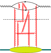
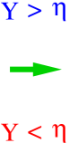
As a first step, we integrate
over gluons with rapidities Y > η 𝑌 𝜂 Y>\eta Y < η 𝑌 𝜂 Y<\eta
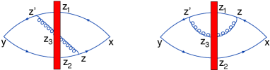
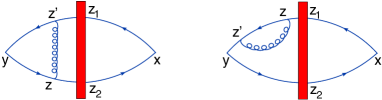
Figure 1: Rapidity factorization. The impact factors with Y > η 𝑌 𝜂 Y>\eta Y < η 𝑌 𝜂 Y<\eta
It is convenient to use the background field formalism: we integrate over gluons with α > σ = e η 𝛼 𝜎 superscript 𝑒 𝜂 \alpha>\sigma=e^{\eta} α < σ 𝛼 𝜎 \alpha<\sigma ( i g ∫ 𝑑 x μ A μ ) 𝑖 𝑔 differential-d subscript 𝑥 𝜇 superscript 𝐴 𝜇 (ig\int\!dx_{\mu}A^{\mu}) ± ∞ plus-or-minus \pm\infty
U x η = Pexp [ i g ∫ − ∞ ∞ 𝑑 u p 1 μ A μ σ ( u p 1 + x ⟂ ) ] , subscript superscript 𝑈 𝜂 𝑥 Pexp delimited-[] 𝑖 𝑔 superscript subscript differential-d 𝑢 superscript subscript 𝑝 1 𝜇 subscript superscript 𝐴 𝜎 𝜇 𝑢 subscript 𝑝 1 subscript 𝑥 perpendicular-to \displaystyle U^{\eta}_{x}~{}=~{}{\rm Pexp}\Big{[}ig\!\int_{-\infty}^{\infty}\!\!du~{}p_{1}^{\mu}A^{\sigma}_{\mu}(up_{1}+x_{\perp})\Big{]},
A μ η ( x ) = ∫ d 4 k θ ( e η − | α k | ) e i k ⋅ x A μ ( k ) subscript superscript 𝐴 𝜂 𝜇 𝑥 superscript 𝑑 4 𝑘 𝜃 superscript 𝑒 𝜂 subscript 𝛼 𝑘 superscript 𝑒 ⋅ 𝑖 𝑘 𝑥 subscript 𝐴 𝜇 𝑘 \displaystyle A^{\eta}_{\mu}(x)~{}=~{}\int\!d^{4}k~{}\theta(e^{\eta}-|\alpha_{k}|)e^{ik\cdot x}A_{\mu}(k) (1)
where the Sudakov variable α k subscript 𝛼 𝑘 \alpha_{k} k = α k p 1 + β k p 2 + k ⟂ 𝑘 subscript 𝛼 𝑘 subscript 𝑝 1 subscript 𝛽 𝑘 subscript 𝑝 2 subscript 𝑘 perpendicular-to k=\alpha_{k}p_{1}+\beta_{k}p_{2}+k_{\perp} p 1 subscript 𝑝 1 p_{1} p 2 subscript 𝑝 2 p_{2} q = p 1 − x B p 2 𝑞 subscript 𝑝 1 subscript 𝑥 𝐵 subscript 𝑝 2 q=p_{1}-x_{B}p_{2} p = p 2 + m N 2 s p 1 𝑝 subscript 𝑝 2 superscript subscript 𝑚 𝑁 2 𝑠 subscript 𝑝 1 p=p_{2}+{m_{N}^{2}\over s}p_{1} q 𝑞 q p 𝑝 p x B = Q 2 / s ≪ 1 subscript 𝑥 𝐵 superscript 𝑄 2 𝑠 much-less-than 1 x_{B}=Q^{2}/s\ll 1 s ≃ 2 p ⋅ q similar-to-or-equals 𝑠 ⋅ 2 𝑝 𝑞 s\simeq 2p\cdot q 2 [ [ \big{[} x 𝑥 x z ] z\big{]} × \times [ [ \big{[} U z ] U_{z}\big{]} × \times [ [ \big{[} z 𝑧 z y ] y\big{]}
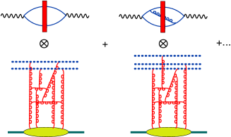
Figure 2: Propagator in a shock-wave background
The explicit form of quark propagator in a shock-wave background can be taken from Ref. npb96
⟨ T { ψ ^ ( x ) ψ ^ ¯ ( y ) } ⟩ A subscript delimited-⟨⟩ 𝑇 ^ 𝜓 𝑥 ¯ ^ 𝜓 𝑦 𝐴 \displaystyle\langle T\{\hat{\psi}(x)\bar{\hat{\psi}}(y)\}\rangle_{A}~{} (2)
= x ∗ > 0 > y ∗ − ∫ d 4 z δ ( z ∗ ) ( x − z ) 2 π 2 ( x − z ) 4 p 2 U z ( z − y ) 2 π 2 ( x − z ) 4 superscript subscript 𝑥 ∗ 0 subscript 𝑦 ∗ absent superscript 𝑑 4 𝑧 𝛿 subscript 𝑧 ∗ 𝑥 𝑧 2 superscript 𝜋 2 superscript 𝑥 𝑧 4 subscript 𝑝 2 subscript 𝑈 𝑧 𝑧 𝑦 2 superscript 𝜋 2 superscript 𝑥 𝑧 4 \displaystyle\stackrel{{\scriptstyle x_{\ast}>0>y_{\ast}}}{{=}}~{}-\!\int\!d^{4}z~{}\delta(z_{\ast}){(\not\!x-\not\!z)\over 2\pi^{2}(x-z)^{4}}\not\!p_{2}U_{z}{(\not\!z-\not\!y)\over 2\pi^{2}(x-z)^{4}}
As usual, we label operators by hats and ⟨ 𝒪 ^ ⟩ A subscript delimited-⟨⟩ ^ 𝒪 𝐴 \langle\hat{\cal O}\rangle_{A} 𝒪 ^ ^ 𝒪 \hat{\cal O} A 𝐴 A x ∗ = p 2 μ x μ = s 2 x + subscript 𝑥 ∗ superscript subscript 𝑝 2 𝜇 subscript 𝑥 𝜇 𝑠 2 superscript 𝑥 x_{\ast}=p_{2}^{\mu}x_{\mu}=\sqrt{s\over 2}x^{+} x ∙ = p 1 μ x μ = s 2 x − subscript 𝑥 ∙ superscript subscript 𝑝 1 𝜇 subscript 𝑥 𝜇 𝑠 2 superscript 𝑥 x_{\bullet}=p_{1}^{\mu}x_{\mu}=\sqrt{s\over 2}x^{-}
x → ρ x ∗ 2 s p 1 + x ∙ 2 s ρ p 2 + x ⟂ , → 𝑥 𝜌 subscript 𝑥 ∗ 2 𝑠 subscript 𝑝 1 subscript 𝑥 ∙ 2 𝑠 𝜌 subscript 𝑝 2 subscript 𝑥 perpendicular-to \displaystyle x~{}\rightarrow~{}\rho x_{\ast}{2\over s}p_{1}+x_{\bullet}{2\over s\rho}p_{2}+x_{\perp},
y → ρ y ∗ 2 s p 1 + y ∙ 2 s ρ p 2 + y ⟂ , → 𝑦 𝜌 subscript 𝑦 ∗ 2 𝑠 subscript 𝑝 1 subscript 𝑦 ∙ 2 𝑠 𝜌 subscript 𝑝 2 subscript 𝑦 perpendicular-to \displaystyle y~{}\rightarrow~{}\rho y_{\ast}{2\over s}p_{1}+y_{\bullet}{2\over s\rho}p_{2}+y_{\perp},~{}~{}~{}~{}~{}~{}~{} (3)
with ρ → ∞ → 𝜌 \rho\rightarrow\infty nlobfklconf ; confamp
The result of the integration over gluons with rapidities Y > η 𝑌 𝜂 Y>\eta 2 3
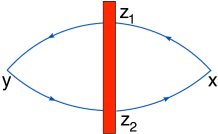
Figure 3: Impact factor in the leading order. Solid lines represent quarks.
⟨ T { ψ ^ ¯ ( x ) γ μ ψ ^ ( x ) ψ ^ ¯ ( y ) γ ν ψ ^ ( y ) } ⟩ A = subscript delimited-⟨⟩ 𝑇 ¯ ^ 𝜓 𝑥 superscript 𝛾 𝜇 ^ 𝜓 𝑥 ¯ ^ 𝜓 𝑦 superscript 𝛾 𝜈 ^ 𝜓 𝑦 𝐴 absent \displaystyle\langle T\{\bar{\hat{\psi}}(x)\gamma^{\mu}\hat{\psi}(x)\bar{\hat{\psi}}(y)\gamma^{\nu}\hat{\psi}(y)\}\rangle_{A}~{}=~{} (4)
= s 2 2 9 π 6 x ∗ 2 y ∗ 2 ∫ d 2 z 1 ⟂ d 2 z 2 ⟂ tr { U z 1 U z 2 † } ( κ ⋅ ζ 1 ) 3 ( κ ⋅ ζ 2 ) 3 absent superscript 𝑠 2 superscript 2 9 superscript 𝜋 6 superscript subscript 𝑥 ∗ 2 superscript subscript 𝑦 ∗ 2 superscript 𝑑 2 subscript 𝑧 perpendicular-to 1 absent superscript 𝑑 2 subscript 𝑧 perpendicular-to 2 absent tr subscript 𝑈 subscript 𝑧 1 subscript superscript 𝑈 † subscript 𝑧 2 superscript ⋅ 𝜅 subscript 𝜁 1 3 superscript ⋅ 𝜅 subscript 𝜁 2 3 \displaystyle=~{}{s^{2}\over 2^{9}\pi^{6}x_{\ast}^{2}y_{\ast}^{2}}\int d^{2}z_{1\perp}d^{2}z_{2\perp}{{\rm tr}\{U_{z_{1}}U^{\dagger}_{z_{2}}\}\over(\kappa\cdot\zeta_{1})^{3}(\kappa\cdot\zeta_{2})^{3}}
× ∂ 2 ∂ x μ ∂ y ν [ 2 ( κ ⋅ ζ 1 ) ( κ ⋅ ζ 2 ) − κ 2 ( ζ 1 ⋅ ζ 2 ) ] + O ( α s ) absent superscript 2 superscript 𝑥 𝜇 superscript 𝑦 𝜈 delimited-[] 2 ⋅ 𝜅 subscript 𝜁 1 ⋅ 𝜅 subscript 𝜁 2 superscript 𝜅 2 ⋅ subscript 𝜁 1 subscript 𝜁 2 𝑂 subscript 𝛼 𝑠 \displaystyle\times~{}{\partial^{2}\over\partial x^{\mu}\partial y^{\nu}}\big{[}2(\kappa\cdot\zeta_{1})(\kappa\cdot\zeta_{2})-\kappa^{2}(\zeta_{1}\cdot\zeta_{2})\big{]}~{}+~{}O(\alpha_{s})
Here we introduced the conformal vectors penecostalba ; penedones
κ = κ x − κ y , κ x = s 2 x ∗ ( p 1 s − x 2 p 2 + x ⟂ ) formulae-sequence 𝜅 subscript 𝜅 𝑥 subscript 𝜅 𝑦 subscript 𝜅 𝑥 𝑠 2 subscript 𝑥 ∗ subscript 𝑝 1 𝑠 superscript 𝑥 2 subscript 𝑝 2 subscript 𝑥 perpendicular-to \displaystyle\kappa~{}=~{}\kappa_{x}-\kappa_{y},~{}~{}~{}~{}~{}\kappa_{x}~{}=~{}{\sqrt{s}\over 2x_{\ast}}({p_{1}\over s}-x^{2}p_{2}+x_{\perp})
ζ i = ( p 1 s + z i ⟂ 2 p 2 + z i ⟂ ) , subscript 𝜁 𝑖 subscript 𝑝 1 𝑠 superscript subscript 𝑧 perpendicular-to 𝑖 absent 2 subscript 𝑝 2 subscript 𝑧 perpendicular-to 𝑖 absent \displaystyle\zeta_{i}~{}=~{}\big{(}{p_{1}\over s}+z_{i\perp}^{2}p_{2}+z_{i\perp}\big{)},~{} (5)
and the notation ℛ ≡ κ 2 ( ζ 1 ⋅ ζ 2 ) 2 ( κ ⋅ ζ 1 ) ( κ ⋅ ζ 2 ) ℛ superscript 𝜅 2 ⋅ subscript 𝜁 1 subscript 𝜁 2 2 ⋅ 𝜅 subscript 𝜁 1 ⋅ 𝜅 subscript 𝜁 2 {\cal R}~{}\equiv~{}{\kappa^{2}(\zeta_{1}\cdot\zeta_{2})\over 2(\kappa\cdot\zeta_{1})(\kappa\cdot\zeta_{2})} ∂ ∂ x μ subscript 𝑥 𝜇 {\partial\over\partial x_{\mu}}
Our goal is the NLO contribution to the r.h.s. of Eq. (4 npb96 ; yura
d d η tr { U ^ z 1 η U ^ z 2 † η } = α s 2 π 2 ∫ d 2 z 3 z 12 2 z 13 2 z 23 2 [ tr { U ^ z 1 η U ^ z 3 † η } \displaystyle{d\over d\eta}{\rm tr}\{\hat{U}^{\eta}_{z_{1}}\hat{U}^{\dagger\eta}_{z_{2}}\}~{}=~{}{\alpha_{s}\over 2\pi^{2}}\!\int\!d^{2}z_{3}~{}{z_{12}^{2}\over z_{13}^{2}z_{23}^{2}}~{}[{\rm tr}\{\hat{U}^{\eta}_{z_{1}}\hat{U}^{\dagger\eta}_{z_{3}}\} (6)
× tr { U ^ z 3 η U ^ z 2 † η } − N c tr { U ^ z 1 η U ^ z 2 † η } ] + NLO contribution \displaystyle\times~{}{\rm tr}\{\hat{U}^{\eta}_{z_{3}}\hat{U}^{\dagger\eta}_{z_{2}}\}-N_{c}{\rm tr}\{\hat{U}^{\eta}_{z_{1}}\hat{U}^{\dagger\eta}_{z_{2}}\}]~{}+~{}{\rm NLO~{}contribution}
(To save space, hereafter z i subscript 𝑧 𝑖 z_{i} z i ⟂ subscript 𝑧 perpendicular-to 𝑖 absent z_{i\perp} z 12 2 ≡ z 12 ⟂ 2 superscript subscript 𝑧 12 2 superscript subscript 𝑧 perpendicular-to 12 absent 2 z_{12}^{2}\equiv z_{12\perp}^{2} nlobk ; nlobksym ; nlolecture prd75 ; kw1
It is worth noting that we performed the OPE program outlined above for scattering of scalar “particles” in 𝒩 = 4 𝒩 4 {\cal N}=4 confamp 𝒩 = 4 𝒩 4 {\cal N}=4 6 solutions α s ( | x − y | ) subscript 𝛼 𝑠 𝑥 𝑦 \alpha_{s}(|x-y|) ∼ | x − y | similar-to absent 𝑥 𝑦 \sim|x-y|
The paper is organized as follows: in Sect. 2 and 3 we calculate the NLO impact factor in the coordinate representation (the results of these Sections were
published previously in Brief Report bfrp k T subscript 𝑘 𝑇 k_{T}
II Calculation of the NLO impact factor
Now we would like to repeat the steps of operator expansion discussed above to the NLO accuracy.
A general form of the expansion of T-product of the electromagnetic currents
in color dipoles looks as follows:
( x − y ) 4 T { ψ ^ ¯ ( x ) γ μ ψ ^ ( x ) ψ ^ ¯ ( y ) γ ν ψ ^ ( y ) } superscript 𝑥 𝑦 4 𝑇 ¯ ^ 𝜓 𝑥 superscript 𝛾 𝜇 ^ 𝜓 𝑥 ¯ ^ 𝜓 𝑦 superscript 𝛾 𝜈 ^ 𝜓 𝑦 \displaystyle(x-y)^{4}T\{\bar{\hat{\psi}}(x)\gamma^{\mu}\hat{\psi}(x)\bar{\hat{\psi}}(y)\gamma^{\nu}\hat{\psi}(y)\}~{}
= ∫ d 2 z 1 d 2 z 2 z 12 4 { I μ ν LO ( z 1 , z 2 ) [ 1 + 3 α s 4 π c F ] tr { U ^ z 1 η U ^ z 2 † η } \displaystyle=~{}\int\!{d^{2}z_{1}d^{2}z_{2}\over z_{12}^{4}}~{}\Big{\{}I_{\mu\nu}^{\rm LO}(z_{1},z_{2})\big{[}1+{3\alpha_{s}\over 4\pi}c_{F}\big{]}{\rm tr}\{\hat{U}^{\eta}_{z_{1}}\hat{U}^{\dagger\eta}_{z_{2}}\}
+ ∫ d 2 z 3 I μ ν NLO ( z 1 , z 2 , z 3 ; η ) superscript 𝑑 2 subscript 𝑧 3 superscript subscript 𝐼 𝜇 𝜈 NLO subscript 𝑧 1 subscript 𝑧 2 subscript 𝑧 3 𝜂 \displaystyle+\int\!d^{2}z_{3}~{}I_{\mu\nu}^{\rm NLO}(z_{1},z_{2},z_{3};\eta)
× [ tr { U ^ z 1 η U ^ z 3 † η } tr { U ^ z 3 η U ^ z 2 † η } − N c tr { U ^ z 1 η U ^ z 2 † η } ] } \displaystyle\times~{}[{\rm tr}\{\hat{U}^{\eta}_{z_{1}}\hat{U}^{\dagger\eta}_{z_{3}}\}{\rm tr}\{\hat{U}^{\eta}_{z_{3}}\hat{U}^{\dagger\eta}_{z_{2}}\}-N_{c}{\rm tr}\{\hat{U}^{\eta}_{z_{1}}\hat{U}^{\dagger\eta}_{z_{2}}\}]\Big{\}} (7)
For simplicity, we calculate at first the impact factor for one flavor of quarks with electric charge one and restore the trivial factor
∑ e i 2 superscript subscript 𝑒 𝑖 2 \sum e_{i}^{2} 77
Unfortunately, in terms of Wilson-line approach there is no direct way to
get the NLO impact factor for the BFKL pomeron. One needs first to find
the coefficient in front of the four-Wilson-line operator (which we will also call the NLO impact factor)
and then linearize it.
The structure of the NLO contribution is clear from the topology of diagrams in the shock-wave background, see Fig. 4 ∼ 1 + 3 α s 4 π c F similar-to absent 1 3 subscript 𝛼 𝑠 4 𝜋 subscript 𝑐 𝐹 \sim~{}1+{3\alpha_{s}\over 4\pi}c_{F} U = 1 𝑈 1 U=1 1 + 3 α s 4 π c F + O ( α s 2 ) 1 3 subscript 𝛼 𝑠 4 𝜋 subscript 𝑐 𝐹 𝑂 superscript subscript 𝛼 𝑠 2 1+{3\alpha_{s}\over 4\pi}c_{F}+O(\alpha_{s}^{2})
In our notations
I μ ν LO ( z 1 , z 2 ) = ℛ 2 π 6 ( κ ⋅ ζ 1 ) ( κ ⋅ ζ 2 ) subscript superscript 𝐼 LO 𝜇 𝜈 subscript 𝑧 1 subscript 𝑧 2 superscript ℛ 2 superscript 𝜋 6 ⋅ 𝜅 subscript 𝜁 1 ⋅ 𝜅 subscript 𝜁 2 \displaystyle I^{\rm LO}_{\mu\nu}(z_{1},z_{2})~{}=~{}{{\cal R}^{2}\over\pi^{6}(\kappa\cdot\zeta_{1})(\kappa\cdot\zeta_{2})}
× ∂ 2 ∂ x μ ∂ y ν [ ( κ ⋅ ζ 1 ) ( κ ⋅ ζ 2 ) − 1 2 κ 2 ( ζ 1 ⋅ ζ 2 ) ] . absent superscript 2 superscript 𝑥 𝜇 superscript 𝑦 𝜈 delimited-[] ⋅ 𝜅 subscript 𝜁 1 ⋅ 𝜅 subscript 𝜁 2 1 2 superscript 𝜅 2 ⋅ subscript 𝜁 1 subscript 𝜁 2 \displaystyle\times~{}{\partial^{2}\over\partial x^{\mu}\partial y^{\nu}}\big{[}(\kappa\cdot\zeta_{1})(\kappa\cdot\zeta_{2})-{1\over 2}\kappa^{2}(\zeta_{1}\cdot\zeta_{2})\big{]}.~{} (8)
which corresponds to the well-known expression for the LO impact factor in the momentum space.
The NLO impact factor is given by the diagrams shown in Fig. 4
Figure 4: Impact factor in the next-to-leading order.
The calculation of these diagrams
is similar to the calculation of the NLO impact factor for scalar currents in 𝒩 = 4 𝒩 4 {\cal N}=4 nlobksym x ∗ > 0 > y ∗ subscript 𝑥 ∗ 0 subscript 𝑦 ∗ x_{\ast}>0>y_{\ast} p 2 μ A μ = 0 superscript subscript 𝑝 2 𝜇 subscript 𝐴 𝜇 0 p_{2}^{\mu}A_{\mu}=0 prd99 ; balbel
⟨ T { A ^ μ a ( x ) A ^ ν b ( y ) } ⟩ = x ∗ > 0 > y ∗ − i 2 ∫ d 4 z δ ( z ∗ ) superscript subscript 𝑥 ∗ 0 subscript 𝑦 ∗ delimited-⟨⟩ 𝑇 subscript superscript ^ 𝐴 𝑎 𝜇 𝑥 subscript superscript ^ 𝐴 𝑏 𝜈 𝑦 𝑖 2 superscript 𝑑 4 𝑧 𝛿 subscript 𝑧 ∗ \displaystyle\langle T\{\hat{A}^{a}_{\mu}(x)\hat{A}^{b}_{\nu}(y)\}\rangle~{}\stackrel{{\scriptstyle x_{\ast}>0>y_{\ast}}}{{=}}~{}-{i\over 2}\int d^{4}z~{}\delta(z_{\ast})~{} (9)
× x ∗ g μ ξ ⟂ − p 2 μ ( x − z ) ξ ⟂ π 2 [ ( x − z ) 2 + i ϵ ] 2 U z ⟂ a b 1 ∂ ∗ ( z ) y ∗ δ ν ⟂ ξ − p 2 ν ( y − z ) ⟂ ξ π 2 [ ( z − y ) 2 + i ϵ ] 2 absent subscript 𝑥 ∗ subscript superscript 𝑔 perpendicular-to 𝜇 𝜉 subscript 𝑝 2 𝜇 subscript superscript 𝑥 𝑧 perpendicular-to 𝜉 superscript 𝜋 2 superscript delimited-[] superscript 𝑥 𝑧 2 𝑖 italic-ϵ 2 subscript superscript 𝑈 𝑎 𝑏 subscript 𝑧 perpendicular-to 1 superscript subscript ∗ 𝑧 subscript 𝑦 subscript superscript 𝛿 perpendicular-to absent 𝜉 𝜈 subscript 𝑝 2 𝜈 superscript subscript 𝑦 𝑧 perpendicular-to 𝜉 superscript 𝜋 2 superscript delimited-[] superscript 𝑧 𝑦 2 𝑖 italic-ϵ 2 \displaystyle\times~{}{x_{\ast}g^{\perp}_{\mu\xi}-p_{2\mu}(x-z)^{\perp}_{\xi}\over\pi^{2}[(x-z)^{2}+i\epsilon]^{2}}\;U^{ab}_{z_{\perp}}{1\over\partial_{\ast}^{(z)}}~{}{y_{*}\delta^{\perp\xi}_{\nu}-p_{2\nu}(y-z)_{\perp}^{\xi}\over\pi^{2}[(z-y)^{2}+i\epsilon]^{2}}
where 1 ∂ ∗ 1 subscript ∗ {1\over\partial_{\ast}} 1 ∂ ∗ + i ϵ 1 subscript ∗ 𝑖 italic-ϵ {1\over\partial_{\ast}+i\epsilon} 1 ∂ ∗ − i ϵ 1 subscript ∗ 𝑖 italic-ϵ {1\over\partial_{\ast}-i\epsilon} 16
The diagrams in Fig. 4
∫ d 4 z x − z ( x − z ) 4 γ μ z − y ( z − y ) 4 z ν z 4 − μ ↔ ν ↔ superscript 𝑑 4 𝑧 𝑥 𝑧 superscript 𝑥 𝑧 4 subscript 𝛾 𝜇 𝑧 𝑦 superscript 𝑧 𝑦 4 subscript 𝑧 𝜈 superscript 𝑧 4 𝜇 𝜈 \displaystyle\int\!d^{4}z~{}{\not\!{x}-\not\!{z}\over(x-z)^{4}}\gamma_{\mu}{\not\!{z}-\not\!{y}\over(z-y)^{4}}{z_{\nu}\over z^{4}}-\mu\leftrightarrow\nu~{}
= π 2 x 2 y 2 ( x − y ) 2 [ − x γ μ y ( x ν x 2 + y ν y 2 ) \displaystyle=~{}{\pi^{2}\over x^{2}y^{2}(x-y)^{2}}\Big{[}-\!\not\!x\gamma_{\mu}\!\not\!y\Big{(}{x_{\nu}\over x^{2}}+{y_{\nu}\over y^{2}}\Big{)}
+ 1 2 ( x γ μ γ ν − γ μ γ ν y ) + 2 x μ y ν x − y ( x − y ) 2 ] − μ ↔ ν \displaystyle+~{}{1\over 2}(\!\not\!x\gamma_{\mu}\gamma_{\nu}-\gamma_{\mu}\gamma_{\nu}\!\not\!y)+2x_{\mu}y_{\nu}{\!\not\!x-\!\not\!y\over(x-y)^{2}}\Big{]}~{}-~{}\mu\leftrightarrow\nu~{}~{}~{} (10)
which gives the 3-point ψ ψ ¯ F μ ν 𝜓 ¯ 𝜓 subscript 𝐹 𝜇 𝜈 \psi\bar{\psi}F_{\mu\nu} g 𝑔 g 2 9 10 z ∙ subscript 𝑧 ∙ z_{\bullet} 4
I μ ν Fig . 4 ( z 1 , z 2 , z 3 ) = I ~ 1 μ ν ( z 1 , z 2 , z 3 ) + I 2 μ ν ( z 1 , z 2 , z 3 ) subscript superscript 𝐼 formulae-sequence Fig 4 𝜇 𝜈 subscript 𝑧 1 subscript 𝑧 2 subscript 𝑧 3 superscript subscript ~ 𝐼 1 𝜇 𝜈 subscript 𝑧 1 subscript 𝑧 2 subscript 𝑧 3 superscript subscript 𝐼 2 𝜇 𝜈 subscript 𝑧 1 subscript 𝑧 2 subscript 𝑧 3 I^{\rm Fig.\ref{fig:nloif}}_{\mu\nu}(z_{1},z_{2},z_{3})~{}=~{}\tilde{I}_{1}^{\mu\nu}(z_{1},z_{2},z_{3})+I_{2}^{\mu\nu}(z_{1},z_{2},z_{3}) (11)
where
I ~ 1 μ ν ( z 1 , z 2 , z 3 ) superscript subscript ~ 𝐼 1 𝜇 𝜈 subscript 𝑧 1 subscript 𝑧 2 subscript 𝑧 3 \displaystyle~{}\tilde{I}_{1}^{\mu\nu}(z_{1},z_{2},z_{3})~{} (12)
= α s 4 π 2 I μ ν LO ( z 1 , z 2 ) ( ζ 1 ⋅ ζ 2 ) ( ζ 1 ⋅ ζ 3 ) ( ζ 1 ⋅ ζ 3 ) ∫ 0 ∞ d α α e i α s 4 σ 𝒵 3 absent subscript 𝛼 𝑠 4 superscript 𝜋 2 subscript superscript 𝐼 LO 𝜇 𝜈 subscript 𝑧 1 subscript 𝑧 2 ⋅ subscript 𝜁 1 subscript 𝜁 2 ⋅ subscript 𝜁 1 subscript 𝜁 3 ⋅ subscript 𝜁 1 subscript 𝜁 3 superscript subscript 0 𝑑 𝛼 𝛼 superscript 𝑒 𝑖 𝛼 𝑠 4 𝜎 subscript 𝒵 3 \displaystyle=~{}{\alpha_{s}\over 4\pi^{2}}I^{\rm LO}_{\mu\nu}(z_{1},z_{2}){(\zeta_{1}\cdot\zeta_{2})\over(\zeta_{1}\cdot\zeta_{3})(\zeta_{1}\cdot\zeta_{3})}\!\int_{0}^{\infty}\!{d\alpha\over\alpha}e^{i\alpha{s\over 4}\sigma{\cal Z}_{3}}
and
( I 2 ) μ ν ( z 1 , z 2 , z 3 ) = α s 16 π 8 ℛ 2 ( κ ⋅ ζ 1 ) ( κ ⋅ ζ 2 ) subscript subscript 𝐼 2 𝜇 𝜈 subscript 𝑧 1 subscript 𝑧 2 subscript 𝑧 3 subscript 𝛼 𝑠 16 superscript 𝜋 8 superscript ℛ 2 ⋅ 𝜅 subscript 𝜁 1 ⋅ 𝜅 subscript 𝜁 2 \displaystyle(I_{2})_{\mu\nu}(z_{1},z_{2},z_{3})~{}=~{}{\alpha_{s}\over 16\pi^{8}}{{\cal R}^{2}\over(\kappa\cdot\zeta_{1})(\kappa\cdot\zeta_{2})} (13)
× { ( κ ⋅ ζ 2 ) ( κ ⋅ ζ 3 ) ∂ 2 ∂ x μ ∂ y ν [ − ( κ ⋅ ζ 1 ) 2 ( ζ 1 ⋅ ζ 3 ) + ( κ ⋅ ζ 1 ) ( κ ⋅ ζ 2 ) ( ζ 2 ⋅ ζ 3 ) \displaystyle\times~{}\Bigg{\{}{(\kappa\cdot\zeta_{2})\over(\kappa\cdot\zeta_{3})}{\partial^{2}\over\partial x^{\mu}\partial y^{\nu}}\Big{[}-{(\kappa\cdot\zeta_{1})^{2}\over(\zeta_{1}\cdot\zeta_{3})}+{(\kappa\cdot\zeta_{1})(\kappa\cdot\zeta_{2})\over(\zeta_{2}\cdot\zeta_{3})}
+ ( κ ⋅ ζ 1 ) ( κ ⋅ ζ 3 ) ( ζ 1 ⋅ ζ 2 ) ( ζ 1 ⋅ ζ 3 ) ( ζ 2 ⋅ ζ 3 ) − κ 2 ( ζ 1 ⋅ ζ 2 ) ( ζ 2 ⋅ ζ 3 ) ] + ( κ ⋅ ζ 2 ) 2 ( κ ⋅ ζ 3 ) 2 \displaystyle+~{}{(\kappa\cdot\zeta_{1})(\kappa\cdot\zeta_{3})(\zeta_{1}\cdot\zeta_{2})\over(\zeta_{1}\cdot\zeta_{3})(\zeta_{2}\cdot\zeta_{3})}-{\kappa^{2}(\zeta_{1}\cdot\zeta_{2})\over(\zeta_{2}\cdot\zeta_{3})}\Big{]}+{(\kappa\cdot\zeta_{2})^{2}\over(\kappa\cdot\zeta_{3})^{2}}
× ∂ 2 ∂ x μ ∂ y ν [ ( κ ⋅ ζ 1 ) ( κ ⋅ ζ 3 ) ( ζ 2 ⋅ ζ 3 ) − κ 2 ( ζ 1 ⋅ ζ 3 ) 2 ( ζ 2 ⋅ ζ 3 ) ] + ( ζ 1 ↔ ζ 2 ) } \displaystyle\times~{}{\partial^{2}\over\partial x^{\mu}\partial y^{\nu}}\Big{[}{(\kappa\cdot\zeta_{1})(\kappa\cdot\zeta_{3})\over(\zeta_{2}\cdot\zeta_{3})}-{\kappa^{2}(\zeta_{1}\cdot\zeta_{3})\over 2(\zeta_{2}\cdot\zeta_{3})}\Big{]}+(\zeta_{1}\leftrightarrow\zeta_{2})\Bigg{\}}
(recall that z i j ⟂ 2 = 2 ( ζ i ⋅ ζ j ) superscript subscript 𝑧 perpendicular-to 𝑖 𝑗 absent 2 2 ⋅ subscript 𝜁 𝑖 subscript 𝜁 𝑗 z_{ij\perp}^{2}=2(\zeta_{i}\cdot\zeta_{j}) 𝒵 i = 4 s ( κ ⋅ ζ i ) subscript 𝒵 𝑖 4 𝑠 ⋅ 𝜅 subscript 𝜁 𝑖 {\cal Z}_{i}={4\over\sqrt{s}}(\kappa\cdot\zeta_{i}) x ∗ > 0 > y ∗ subscript 𝑥 ∗ 0 subscript 𝑦 ∗ x_{\ast}>0>y_{\ast} x ∗ < 0 < y ∗ subscript 𝑥 ∗ 0 subscript 𝑦 ∗ x_{\ast}<0<y_{\ast}
The integral over α 𝛼 \alpha 12 4 7 7 ⟨ U ^ z 3 ⟩ A = U z 3 subscript delimited-⟨⟩ subscript ^ 𝑈 subscript 𝑧 3 𝐴 subscript 𝑈 subscript 𝑧 3 \langle\hat{U}_{z_{3}}\rangle_{A}=U_{z_{3}}
⟨ T { ψ ^ ¯ ( x ) γ μ ψ ^ ( x ) ψ ^ ¯ ( y ) γ ν ψ ^ ( y ) } ⟩ A subscript delimited-⟨⟩ 𝑇 ¯ ^ 𝜓 𝑥 superscript 𝛾 𝜇 ^ 𝜓 𝑥 ¯ ^ 𝜓 𝑦 superscript 𝛾 𝜈 ^ 𝜓 𝑦 𝐴 \displaystyle\langle T\{\bar{\hat{\psi}}(x)\gamma^{\mu}\hat{\psi}(x)\bar{\hat{\psi}}(y)\gamma^{\nu}\hat{\psi}(y)\}\rangle_{A}~{}
− ∫ d 2 z 1 d 2 z 2 z 12 4 I μ ν LO ( x , y ; z 1 , z 2 ) ⟨ tr { U ^ z 1 η U ^ z 2 † η } ⟩ A superscript 𝑑 2 subscript 𝑧 1 superscript 𝑑 2 subscript 𝑧 2 superscript subscript 𝑧 12 4 superscript subscript 𝐼 𝜇 𝜈 LO 𝑥 𝑦 subscript 𝑧 1 subscript 𝑧 2 subscript delimited-⟨⟩ tr subscript superscript ^ 𝑈 𝜂 subscript 𝑧 1 subscript superscript ^ 𝑈 † absent 𝜂 subscript 𝑧 2 𝐴 \displaystyle-\int\!{d^{2}z_{1}d^{2}z_{2}\over z_{12}^{4}}~{}I_{\mu\nu}^{\rm LO}(x,y;z_{1},z_{2})\langle{\rm tr}\{\hat{U}^{\eta}_{z_{1}}\hat{U}^{\dagger\eta}_{z_{2}}\}\rangle_{A}
= ∫ d 2 z 1 d 2 z 2 z 12 4 d 2 z 3 I μ ν NLO ( x , y ; z 1 , z 2 , z 3 ; η ) absent superscript 𝑑 2 subscript 𝑧 1 superscript 𝑑 2 subscript 𝑧 2 superscript subscript 𝑧 12 4 superscript 𝑑 2 subscript 𝑧 3 superscript subscript 𝐼 𝜇 𝜈 NLO 𝑥 𝑦 subscript 𝑧 1 subscript 𝑧 2 subscript 𝑧 3 𝜂 \displaystyle=~{}\int\!{d^{2}z_{1}d^{2}z_{2}\over z_{12}^{4}}d^{2}z_{3}~{}I_{\mu\nu}^{\rm NLO}(x,y;z_{1},z_{2},z_{3};\eta)
[ tr { U z 1 U z 3 † } tr { U z 3 U z 2 † } − N c tr { U z 1 U z 2 † } ] delimited-[] tr subscript 𝑈 subscript 𝑧 1 subscript superscript 𝑈 † subscript 𝑧 3 tr subscript 𝑈 subscript 𝑧 3 subscript superscript 𝑈 † subscript 𝑧 2 subscript 𝑁 𝑐 tr subscript 𝑈 subscript 𝑧 1 subscript superscript 𝑈 † subscript 𝑧 2 \displaystyle[{\rm tr}\{U_{z_{1}}U^{\dagger}_{z_{3}}\}{\rm tr}\{U_{z_{3}}U^{\dagger}_{z_{2}}\}-N_{c}{\rm tr}\{U_{z_{1}}U^{\dagger}_{z_{2}}\}] (14)
The NLO matrix element ⟨ T { ψ ^ ¯ ( x ) γ μ ψ ^ ( x ) ψ ^ ¯ ( y ) γ ν ψ ^ ( y ) } ⟩ A subscript delimited-⟨⟩ 𝑇 ¯ ^ 𝜓 𝑥 superscript 𝛾 𝜇 ^ 𝜓 𝑥 ¯ ^ 𝜓 𝑦 superscript 𝛾 𝜈 ^ 𝜓 𝑦 𝐴 \langle T\{\bar{\hat{\psi}}(x)\gamma^{\mu}\hat{\psi}(x)\bar{\hat{\psi}}(y)\gamma^{\nu}\hat{\psi}(y)\}\rangle_{A} 11
α s 2 π 2 ∫ d 2 z 1 d 2 z 2 z 12 4 I μ ν LO ( z 1 , z 2 ) ∫ 0 σ d α α ∫ d 2 z 3 z 12 2 z 13 2 z 23 2 subscript 𝛼 𝑠 2 superscript 𝜋 2 superscript 𝑑 2 subscript 𝑧 1 superscript 𝑑 2 subscript 𝑧 2 superscript subscript 𝑧 12 4 superscript subscript 𝐼 𝜇 𝜈 LO subscript 𝑧 1 subscript 𝑧 2 superscript subscript 0 𝜎 𝑑 𝛼 𝛼 superscript 𝑑 2 subscript 𝑧 3 superscript subscript 𝑧 12 2 superscript subscript 𝑧 13 2 superscript subscript 𝑧 23 2 \displaystyle{\alpha_{s}\over 2\pi^{2}}\!\int\!{d^{2}z_{1}d^{2}z_{2}\over z_{12}^{4}}~{}I_{\mu\nu}^{\rm LO}(z_{1},z_{2})\!\int_{0}^{\sigma}\!{d\alpha\over\alpha}\!\int\!d^{2}z_{3}~{}{z_{12}^{2}\over z_{13}^{2}z_{23}^{2}}
× [ tr { U z 1 U z 3 † } tr { U z 3 U z 2 † } − N c tr { U z 1 U z 2 † } ] absent delimited-[] tr subscript 𝑈 subscript 𝑧 1 subscript superscript 𝑈 † subscript 𝑧 3 tr subscript 𝑈 subscript 𝑧 3 subscript superscript 𝑈 † subscript 𝑧 2 subscript 𝑁 𝑐 tr subscript 𝑈 subscript 𝑧 1 subscript superscript 𝑈 † subscript 𝑧 2 \displaystyle\times~{}~{}[{\rm tr}\{U_{z_{1}}U^{\dagger}_{z_{3}}\}{\rm tr}\{U_{z_{3}}U^{\dagger}_{z_{2}}\}-~{}N_{c}{\rm tr}\{U_{z_{1}}U^{\dagger}_{z_{2}}\}] (15)
as follows from Eq. (6 α 𝛼 \alpha σ = e η 𝜎 superscript 𝑒 𝜂 \sigma=e^{\eta} U ^ η superscript ^ 𝑈 𝜂 \hat{U}^{\eta} 1 15 11
I μ ν NLO ( z 1 , z 2 , z 3 ; η ) = I 1 μ ν ( z 1 , z 2 , z 3 ; η ) + I 2 μ ν ( z 1 , z 2 , z 3 ) , subscript superscript 𝐼 NLO 𝜇 𝜈 subscript 𝑧 1 subscript 𝑧 2 subscript 𝑧 3 𝜂 superscript subscript 𝐼 1 𝜇 𝜈 subscript 𝑧 1 subscript 𝑧 2 subscript 𝑧 3 𝜂 superscript subscript 𝐼 2 𝜇 𝜈 subscript 𝑧 1 subscript 𝑧 2 subscript 𝑧 3 \displaystyle I^{\rm NLO}_{\mu\nu}(z_{1},z_{2},z_{3};\eta)~{}=~{}I_{1}^{\mu\nu}(z_{1},z_{2},z_{3};\eta)+I_{2}^{\mu\nu}(z_{1},z_{2},z_{3}),
I 1 μ ν ( x , y ; z 1 , z 2 , z 3 ; η ) superscript subscript 𝐼 1 𝜇 𝜈 𝑥 𝑦 subscript 𝑧 1 subscript 𝑧 2 subscript 𝑧 3 𝜂 \displaystyle I_{1}^{\mu\nu}(x,y;z_{1},z_{2},z_{3};\eta)~{}
= α s 2 π 2 I μ ν LO ( z 1 , z 2 ) z 12 2 z 13 2 z 23 2 [ ∫ 0 ∞ d α α e i α s 4 𝒵 3 − ∫ 0 σ d α α ] absent subscript 𝛼 𝑠 2 superscript 𝜋 2 subscript superscript 𝐼 LO 𝜇 𝜈 subscript 𝑧 1 subscript 𝑧 2 superscript subscript 𝑧 12 2 superscript subscript 𝑧 13 2 superscript subscript 𝑧 23 2 delimited-[] superscript subscript 0 𝑑 𝛼 𝛼 superscript 𝑒 𝑖 𝛼 𝑠 4 subscript 𝒵 3 superscript subscript 0 𝜎 𝑑 𝛼 𝛼 \displaystyle=~{}{\alpha_{s}\over 2\pi^{2}}I^{\rm LO}_{\mu\nu}(z_{1},z_{2}){z_{12}^{2}\over z_{13}^{2}z_{23}^{2}}\Big{[}\!\int_{0}^{\infty}\!{d\alpha\over\alpha}~{}e^{i\alpha{s\over 4}{\cal Z}_{3}}-\!\int_{0}^{\sigma}\!{d\alpha\over\alpha}\Big{]}
= − α s 2 π 2 I μ ν LO z 12 2 z 13 2 z 23 2 [ ln σ s 4 𝒵 3 − i π 2 + C ] absent subscript 𝛼 𝑠 2 superscript 𝜋 2 subscript superscript 𝐼 LO 𝜇 𝜈 superscript subscript 𝑧 12 2 superscript subscript 𝑧 13 2 superscript subscript 𝑧 23 2 delimited-[] 𝜎 𝑠 4 subscript 𝒵 3 𝑖 𝜋 2 𝐶 \displaystyle=~{}-{\alpha_{s}\over 2\pi^{2}}I^{\rm LO}_{\mu\nu}{z_{12}^{2}\over z_{13}^{2}z_{23}^{2}}\big{[}\ln{\sigma s\over 4}{\cal Z}_{3}-{i\pi\over 2}+C\big{]} (16)
where C 𝐶 C 4 nlobk ; confamp ; nlolecture α < σ 𝛼 𝜎 \alpha<\sigma ∼ ln σ 𝒵 3 similar-to absent 𝜎 subscript 𝒵 3 \sim\ln\sigma{\cal Z}_{3} 16
[ tr { U ^ z 1 U ^ z 2 † } ] a subscript delimited-[] tr subscript ^ 𝑈 subscript 𝑧 1 subscript superscript ^ 𝑈 † subscript 𝑧 2 𝑎 \displaystyle[{\rm tr}\{\hat{U}_{z_{1}}\hat{U}^{\dagger}_{z_{2}}\}\big{]}_{a}~{} (17)
= tr { U ^ z 1 σ U ^ z 2 † σ } + α s 2 π 2 ∫ d 2 z 3 z 12 2 z 13 2 z 23 2 [ tr { U ^ z 1 σ U ^ z 3 † σ } \displaystyle=~{}{\rm tr}\{\hat{U}^{\sigma}_{z_{1}}\hat{U}^{\dagger\sigma}_{z_{2}}\}+~{}{\alpha_{s}\over 2\pi^{2}}\!\int\!d^{2}z_{3}~{}{z_{12}^{2}\over z_{13}^{2}z_{23}^{2}}[{\rm tr}\{\hat{U}^{\sigma}_{z_{1}}\hat{U}^{\dagger\sigma}_{z_{3}}\}
× tr { U ^ z 3 σ U ^ z 2 † σ } − N c tr { U ^ z 1 σ U ^ z 2 † σ } ] ln 4 a z 12 2 σ 2 s z 13 2 z 23 2 + O ( α s 2 ) \displaystyle\times~{}{\rm tr}\{\hat{U}^{\sigma}_{z_{3}}\hat{U}^{\dagger\sigma}_{z_{2}}\}-N_{c}{\rm tr}\{\hat{U}^{\sigma}_{z_{1}}\hat{U}^{\dagger\sigma}_{z_{2}}\}]\ln{4az_{12}^{2}\over\sigma^{2}sz_{13}^{2}z_{23}^{2}}~{}+~{}O(\alpha_{s}^{2})
where a 𝑎 a a → a e − 2 η → 𝑎 𝑎 superscript 𝑒 2 𝜂 a\rightarrow ae^{-2\eta} [ tr { U ^ z 1 σ U ^ z 2 † σ } ] a conf superscript subscript delimited-[] tr subscript superscript ^ 𝑈 𝜎 subscript 𝑧 1 subscript superscript ^ 𝑈 † absent 𝜎 subscript 𝑧 2 𝑎 conf [{\rm tr}\{\hat{U}^{\sigma}_{z_{1}}\hat{U}^{\dagger\sigma}_{z_{2}}\}\big{]}_{a}^{\rm conf} η = ln σ 𝜂 𝜎 \eta=\ln\sigma a 𝑎 a d d η [ tr { U ^ z 1 U ^ z 2 † } ] a conf = 0 𝑑 𝑑 𝜂 superscript subscript delimited-[] tr subscript ^ 𝑈 subscript 𝑧 1 subscript superscript ^ 𝑈 † subscript 𝑧 2 𝑎 conf 0 {d\over d\eta}[{\rm tr}\{\hat{U}_{z_{1}}\hat{U}^{\dagger}_{z_{2}}\}\big{]}_{a}^{\rm conf}~{}=~{}0 d d a [ tr { U ^ z 1 U ^ z 2 † } ] a conf 𝑑 𝑑 𝑎 superscript subscript delimited-[] tr subscript ^ 𝑈 subscript 𝑧 1 subscript superscript ^ 𝑈 † subscript 𝑧 2 𝑎 conf {d\over da}[{\rm tr}\{\hat{U}_{z_{1}}\hat{U}^{\dagger}_{z_{2}}\}\big{]}_{a}^{\rm conf} O ( α s 2 ) 𝑂 superscript subscript 𝛼 𝑠 2 O(\alpha_{s}^{2}) nlobksym ; nlolecture
Rewritten in terms of composite dipoles (17 7
T { ψ ^ ¯ ( x ) γ μ ψ ^ ( x ) ψ ^ ¯ ( y ) γ ν ψ ^ ( y ) } 𝑇 ¯ ^ 𝜓 𝑥 superscript 𝛾 𝜇 ^ 𝜓 𝑥 ¯ ^ 𝜓 𝑦 superscript 𝛾 𝜈 ^ 𝜓 𝑦 \displaystyle T\{\bar{\hat{\psi}}(x)\gamma^{\mu}\hat{\psi}(x)\bar{\hat{\psi}}(y)\gamma^{\nu}\hat{\psi}(y)\}~{}
= ∫ d 2 z 1 d 2 z 2 z 12 4 { I μ ν LO ( z 1 , z 2 ) [ 1 + 3 α s 4 π c F ] [ tr { U ^ z 1 U ^ z 2 † } ] a \displaystyle=~{}\int\!{d^{2}z_{1}d^{2}z_{2}\over z_{12}^{4}}~{}\Big{\{}I_{\mu\nu}^{\rm LO}(z_{1},z_{2})\big{[}1+{3\alpha_{s}\over 4\pi}c_{F}\big{]}[{\rm tr}\{\hat{U}_{z_{1}}\hat{U}^{\dagger}_{z_{2}}\}]_{a}
+ ∫ d 2 z 3 I μ ν NLO ( z 1 , z 2 , z 3 ; a ) superscript 𝑑 2 subscript 𝑧 3 superscript subscript 𝐼 𝜇 𝜈 NLO subscript 𝑧 1 subscript 𝑧 2 subscript 𝑧 3 𝑎 \displaystyle+\int\!d^{2}z_{3}~{}I_{\mu\nu}^{\rm NLO}(z_{1},z_{2},z_{3};a)
× [ tr { U ^ z 1 U ^ z 3 † } tr { U ^ z 3 U ^ z 2 † } − N c tr { U ^ z 1 U ^ z 2 † } ] a } \displaystyle\times~{}[{\rm tr}\{\hat{U}_{z_{1}}\hat{U}^{\dagger}_{z_{3}}\}{\rm tr}\{\hat{U}_{z_{3}}\hat{U}^{\dagger}_{z_{2}}\}-N_{c}{\rm tr}\{\hat{U}_{z_{1}}\hat{U}^{\dagger}_{z_{2}}\}]_{a}\Big{\}} (18)
We need to choose the “new rapidity cutoff” a 𝑎 a a 𝑎 a a 0 = − κ − 2 + i ϵ = − 4 x ∗ y ∗ s ( x − y ) 2 + i ϵ subscript 𝑎 0 superscript 𝜅 2 𝑖 italic-ϵ 4 subscript 𝑥 ∗ subscript 𝑦 ∗ 𝑠 superscript 𝑥 𝑦 2 𝑖 italic-ϵ a_{0}=-\kappa^{-2}+i\epsilon=-{4x_{\ast}y_{\ast}\over s(x-y)^{2}}+i\epsilon
( x − y ) 4 T { ψ ^ ¯ ( x ) γ μ ψ ^ ( x ) ψ ^ ¯ ( y ) γ ν ψ ^ ( y ) } superscript 𝑥 𝑦 4 𝑇 ¯ ^ 𝜓 𝑥 superscript 𝛾 𝜇 ^ 𝜓 𝑥 ¯ ^ 𝜓 𝑦 superscript 𝛾 𝜈 ^ 𝜓 𝑦 \displaystyle(x-y)^{4}T\{\bar{\hat{\psi}}(x)\gamma^{\mu}\hat{\psi}(x)\bar{\hat{\psi}}(y)\gamma^{\nu}\hat{\psi}(y)\}~{} (19)
= ∫ d 2 z 1 d 2 z 2 z 12 4 { I LO μ ν ( z 1 , z 2 ) [ 1 + 3 α s 4 π c F ] [ tr { U ^ z 1 U ^ z 2 † } ] a 0 \displaystyle=\int\!{d^{2}z_{1}d^{2}z_{2}\over z_{12}^{4}}~{}\Big{\{}I^{\mu\nu}_{\rm LO}(z_{1},z_{2})\big{[}1+{3\alpha_{s}\over 4\pi}c_{F}\big{]}[{\rm tr}\{\hat{U}_{z_{1}}\hat{U}^{\dagger}_{z_{2}}\}]_{a_{0}}
+ ∫ d 2 z 3 [ α s 4 π 2 z 12 2 z 13 2 z 23 2 ( ln κ 2 ( ζ 1 ⋅ ζ 3 ) ( ζ 1 ⋅ ζ 3 ) 2 ( κ ⋅ ζ 3 ) 2 ( ζ 1 ⋅ ζ 2 ) − 2 C ) I LO μ ν \displaystyle+\int\!d^{2}z_{3}\Big{[}{\alpha_{s}\over 4\pi^{2}}{z_{12}^{2}\over z_{13}^{2}z_{23}^{2}}\Big{(}\ln{\kappa^{2}(\zeta_{1}\cdot\zeta_{3})(\zeta_{1}\cdot\zeta_{3})\over 2(\kappa\cdot\zeta_{3})^{2}(\zeta_{1}\cdot\zeta_{2})}-2C\Big{)}I^{\mu\nu}_{\rm LO}
+ I 2 μ ν ] [ tr { U ^ z 1 U ^ z 3 † } tr { U ^ z 3 U ^ z 2 † } − N c tr { U ^ z 1 U ^ z 2 † } ] a 0 } \displaystyle+~{}I_{2}^{\mu\nu}\Big{]}[{\rm tr}\{\hat{U}_{z_{1}}\hat{U}^{\dagger}_{z_{3}}\}{\rm tr}\{\hat{U}_{z_{3}}\hat{U}^{\dagger}_{z_{2}}\}-N_{c}{\rm tr}\{\hat{U}_{z_{1}}\hat{U}^{\dagger}_{z_{2}}\}]_{a_{0}}\Big{\}}
Here the composite dipole [ tr { U ^ z 1 σ U ^ z 2 † σ } ] a 0 subscript delimited-[] tr subscript superscript ^ 𝑈 𝜎 subscript 𝑧 1 subscript superscript ^ 𝑈 † absent 𝜎 subscript 𝑧 2 subscript 𝑎 0 [{\rm tr}\{\hat{U}^{\sigma}_{z_{1}}\hat{U}^{\dagger\sigma}_{z_{2}}\}]_{a_{0}} 17 a 0 = − 4 x ∗ y ∗ s ( x − y ) 2 + i ϵ subscript 𝑎 0 4 subscript 𝑥 ∗ subscript 𝑦 ∗ 𝑠 superscript 𝑥 𝑦 2 𝑖 italic-ϵ a_{0}=-{4x_{\ast}y_{\ast}\over s(x-y)^{2}}+i\epsilon I LO μ ν ( z 1 , z 2 ) subscript superscript 𝐼 𝜇 𝜈 LO subscript 𝑧 1 subscript 𝑧 2 I^{\mu\nu}_{\rm LO}(z_{1},z_{2}) I 2 μ ν ( z 1 , z 2 , z 3 ) superscript subscript 𝐼 2 𝜇 𝜈 subscript 𝑧 1 subscript 𝑧 2 subscript 𝑧 3 I_{2}^{\mu\nu}(z_{1},z_{2},z_{3}) 8 13
III NLO impact factor for the BFKL pomeron
For the studies of DIS with the linear NLO BFKL equation (up to two-gluon accuracy) we need the linearized version of Eq. (19
𝒰 ^ a ( z 1 , z 2 ) = 1 − 1 N c [ tr { U ^ z 1 U ^ z 2 † } ] a subscript ^ 𝒰 𝑎 subscript 𝑧 1 subscript 𝑧 2 1 1 subscript 𝑁 𝑐 subscript delimited-[] tr subscript ^ 𝑈 subscript 𝑧 1 subscript superscript ^ 𝑈 † subscript 𝑧 2 𝑎 \hat{\cal U}_{a}(z_{1},z_{2})=1-{1\over N_{c}}[{\rm tr}\{\hat{U}_{z_{1}}\hat{U}^{\dagger}_{z_{2}}\}]_{a} (20)
and consider the linearization
1 N c 2 tr { U ^ z 1 U ^ z 3 † } tr { U ^ z 3 U ^ z 2 † } − 1 N c tr { U ^ z 1 U ^ z 2 † } ] a 0 \displaystyle{1\over N_{c}^{2}}{\rm tr}\{\hat{U}_{z_{1}}\hat{U}^{\dagger}_{z_{3}}\}{\rm tr}\{\hat{U}_{z_{3}}\hat{U}^{\dagger}_{z_{2}}\}-{1\over N_{c}}{\rm tr}\{\hat{U}_{z_{1}}\hat{U}^{\dagger}_{z_{2}}\}]_{a_{0}}~{}
≃ 𝒰 ^ ( z 1 , z 2 ) − 𝒰 ^ ( z 1 , z 3 ) − 𝒰 ^ ( z 2 , z 3 ) similar-to-or-equals absent ^ 𝒰 subscript 𝑧 1 subscript 𝑧 2 ^ 𝒰 subscript 𝑧 1 subscript 𝑧 3 ^ 𝒰 subscript 𝑧 2 subscript 𝑧 3 \displaystyle\simeq~{}\hat{\cal U}(z_{1},z_{2})-\hat{\cal U}(z_{1},z_{3})-\hat{\cal U}(z_{2},z_{3})
one of the integrals over z i subscript 𝑧 𝑖 z_{i} 19
1 N c ( x − y ) 4 T { ψ ^ ¯ ( x ) γ μ ψ ^ ( x ) ψ ^ ¯ ( y ) γ ν ψ ^ ( y ) } 1 subscript 𝑁 𝑐 superscript 𝑥 𝑦 4 𝑇 ¯ ^ 𝜓 𝑥 superscript 𝛾 𝜇 ^ 𝜓 𝑥 ¯ ^ 𝜓 𝑦 superscript 𝛾 𝜈 ^ 𝜓 𝑦 \displaystyle{1\over N_{c}}(x-y)^{4}T\{\bar{\hat{\psi}}(x)\gamma^{\mu}\hat{\psi}(x)\bar{\hat{\psi}}(y)\gamma^{\nu}\hat{\psi}(y)\}~{} (21)
= ∂ κ α ∂ x μ ∂ κ β ∂ y ν ∫ d z 1 d z 2 z 12 4 𝒰 ^ a 0 ( z 1 , z 2 ) [ ℐ α β LO ( 1 + α s π ) + ℐ α β NLO ] absent superscript 𝜅 𝛼 superscript 𝑥 𝜇 superscript 𝜅 𝛽 superscript 𝑦 𝜈 𝑑 subscript 𝑧 1 𝑑 subscript 𝑧 2 superscript subscript 𝑧 12 4 subscript ^ 𝒰 subscript 𝑎 0 subscript 𝑧 1 subscript 𝑧 2 delimited-[] superscript subscript ℐ 𝛼 𝛽 LO 1 subscript 𝛼 𝑠 𝜋 superscript subscript ℐ 𝛼 𝛽 NLO \displaystyle=~{}{\partial\kappa^{\alpha}\over\partial x^{\mu}}{\partial\kappa^{\beta}\over\partial y^{\nu}}\!\int\!{dz_{1}dz_{2}\over z_{12}^{4}}~{}\hat{\cal U}_{a_{0}}(z_{1},z_{2})\big{[}{\cal I}_{\alpha\beta}^{\rm LO}\big{(}1+{\alpha_{s}\over\pi}\big{)}+{\cal I}_{\alpha\beta}^{\rm NLO}\big{]}
where
ℐ LO α β ( x , y ; z 1 , z 2 ) = ℛ 2 g α β ( ζ 1 ⋅ ζ 2 ) − ζ 1 α ζ 2 β − ζ 2 α ζ 1 β π 6 ( κ ⋅ ζ 1 ) ( κ ⋅ ζ 2 ) subscript superscript ℐ 𝛼 𝛽 LO 𝑥 𝑦 subscript 𝑧 1 subscript 𝑧 2 superscript ℛ 2 superscript 𝑔 𝛼 𝛽 ⋅ subscript 𝜁 1 subscript 𝜁 2 superscript subscript 𝜁 1 𝛼 superscript subscript 𝜁 2 𝛽 superscript subscript 𝜁 2 𝛼 superscript subscript 𝜁 1 𝛽 superscript 𝜋 6 ⋅ 𝜅 subscript 𝜁 1 ⋅ 𝜅 subscript 𝜁 2 {\cal I}^{\alpha\beta}_{\rm LO}(x,y;z_{1},z_{2})~{}=~{}{\cal R}^{2}{g^{\alpha\beta}(\zeta_{1}\cdot\zeta_{2})-\zeta_{1}^{\alpha}\zeta_{2}^{\beta}-\zeta_{2}^{\alpha}\zeta_{1}^{\beta}\over\pi^{6}(\kappa\cdot\zeta_{1})(\kappa\cdot\zeta_{2})} (22)
(see Eq. (8
ℐ NLO α β ( x , y ; z 1 , z 2 ) = α s N c 4 π 7 ℛ 2 { ζ 1 α ζ 2 β + ζ 1 ↔ ζ 2 ( κ ⋅ ζ 1 ) ( κ ⋅ ζ 2 ) \displaystyle{\cal I}^{\alpha\beta}_{\rm NLO}(x,y;z_{1},z_{2})~{}=~{}{\alpha_{s}N_{c}\over 4\pi^{7}}{\cal R}^{2}\Bigg{\{}{\zeta_{1}^{\alpha}\zeta_{2}^{\beta}+\zeta_{1}\leftrightarrow\zeta_{2}\over(\kappa\cdot\zeta_{1})(\kappa\cdot\zeta_{2})}
× [ 4 L i 2 ( 1 − ℛ ) − 2 π 2 3 + 2 ln ℛ 1 − ℛ + ln ℛ ℛ − 4 ln ℛ + 1 2 ℛ \displaystyle\times~{}\Big{[}4{\rm Li}_{2}(1-{\cal R})-{2\pi^{2}\over 3}+{2\ln{\cal R}\over 1-{\cal R}}+{\ln{\cal R}\over{\cal R}}-4\ln{\cal R}+{1\over 2{\cal R}}
− 2 + 2 ( ln 1 ℛ + 1 ℛ − 2 ) ( ln 1 ℛ + 2 C ) − 4 C − 2 C ℛ ] \displaystyle-~{}2+2(\ln{1\over{\cal R}}+{1\over{\cal R}}-2)\big{(}\ln{1\over{\cal R}}+2C\big{)}-4C-{2C\over{\cal R}}\Big{]}
+ ( ζ 1 α ζ 1 β ( κ ⋅ ζ 1 ) 2 + ζ 1 ↔ ζ 2 ) [ ln ℛ ℛ − 2 C ℛ + 2 ln ℛ 1 − ℛ − 1 2 ℛ ] \displaystyle+\Big{(}{\zeta_{1}^{\alpha}\zeta_{1}^{\beta}\over(\kappa\cdot\zeta_{1})^{2}}+\zeta_{1}\leftrightarrow\zeta_{2}\Big{)}\Big{[}{\ln{\cal R}\over{\cal R}}-{2C\over{\cal R}}+2{\ln{\cal R}\over 1-{\cal R}}-{1\over 2{\cal R}}\Big{]}
+ [ ζ 1 α κ β + ζ 1 β κ α ( κ ⋅ ζ 1 ) κ 2 + ζ 1 ↔ ζ 2 ] [ − 2 ln ℛ 1 − ℛ − ln ℛ ℛ \displaystyle+~{}\Big{[}{\zeta_{1}^{\alpha}\kappa^{\beta}+\zeta_{1}^{\beta}\kappa^{\alpha}\over(\kappa\cdot\zeta_{1})\kappa^{2}}+\zeta_{1}\leftrightarrow\zeta_{2}\Big{]}\Big{[}-2{\ln{\cal R}\over 1-{\cal R}}-{\ln{\cal R}\over{\cal R}}
+ ln ℛ − 3 2 ℛ + 5 2 + 2 C + 2 C ℛ ] − 2 κ 2 ( g α β − 2 κ α κ β κ 2 ) \displaystyle+\ln{\cal R}-{3\over 2{\cal R}}+{5\over 2}+2C+{2C\over{\cal R}}\Big{]}-{2\over\kappa^{2}}\Big{(}g^{\alpha\beta}-2{\kappa^{\alpha}\kappa^{\beta}\over\kappa^{2}}\Big{)}
+ g α β ( ζ 1 ⋅ ζ 2 ) ( κ ⋅ ζ 1 ) ( κ ⋅ ζ 2 ) [ 2 π 2 3 − 4 L i 2 ( 1 − ℛ ) − 2 ( ln 1 ℛ + 1 ℛ \displaystyle+~{}{g^{\alpha\beta}(\zeta_{1}\cdot\zeta_{2})\over(\kappa\cdot\zeta_{1})(\kappa\cdot\zeta_{2})}\Big{[}{2\pi^{2}\over 3}-4{\rm Li}_{2}(1-{\cal R})-2\big{(}\ln{1\over{\cal R}}+{1\over{\cal R}}
+ 1 2 ℛ 2 − 3 ) ( ln 1 ℛ + 2 C ) + 6 ln ℛ − 2 ℛ + 2 + 3 2 ℛ 2 ] } \displaystyle+~{}{1\over 2{\cal R}^{2}}-3\big{)}\big{(}\ln{1\over{\cal R}}+2C\big{)}+6\ln{\cal R}-{2\over{\cal R}}+2+{3\over 2{\cal R}^{2}}\Big{]}\Bigg{\}}
(23)
where Li( z ) 2 {}_{2}(z) penecostalba2
While it is easy to see that
d d x μ 1 ( x − y ) 4 ∂ κ α ∂ x μ ∂ κ β ∂ y ν ℐ α β LO ( x , y ; z i ) = 0 𝑑 𝑑 subscript 𝑥 𝜇 1 superscript 𝑥 𝑦 4 superscript 𝜅 𝛼 superscript 𝑥 𝜇 superscript 𝜅 𝛽 superscript 𝑦 𝜈 superscript subscript ℐ 𝛼 𝛽 LO 𝑥 𝑦 subscript 𝑧 𝑖 0 \displaystyle{d\over dx_{\mu}}{1\over(x-y)^{4}}{\partial\kappa^{\alpha}\over\partial x^{\mu}}{\partial\kappa^{\beta}\over\partial y^{\nu}}{\cal I}_{\alpha\beta}^{\rm LO}(x,y;z_{i})~{}=~{}0 (24)
one should be careful when checking the electromagnetic gauge invariance in the next-to-leading order. The reason is that
the composite dipole 𝒰 ^ a 0 ( z 1 , z 2 ) superscript ^ 𝒰 subscript 𝑎 0 subscript 𝑧 1 subscript 𝑧 2 \hat{\cal U}^{a_{0}}(z_{1},z_{2}) x 𝑥 x a 0 = − 4 x ∗ y ∗ s ( x − y ) 2 subscript 𝑎 0 4 subscript 𝑥 ∗ subscript 𝑦 ∗ 𝑠 superscript 𝑥 𝑦 2 a_{0}=-{4x_{\ast}y_{\ast}\over s(x-y)^{2}} 21
∂ ∂ x μ 1 ( x − y ) 4 ∂ κ α ∂ x μ ∂ κ β ∂ y ν ∫ d z 1 d z 2 z 12 4 𝒰 ^ a 0 ( z 1 , z 2 ) ℐ α β NLO ( x , y ; z i ) subscript 𝑥 𝜇 1 superscript 𝑥 𝑦 4 superscript 𝜅 𝛼 superscript 𝑥 𝜇 superscript 𝜅 𝛽 superscript 𝑦 𝜈 𝑑 subscript 𝑧 1 𝑑 subscript 𝑧 2 superscript subscript 𝑧 12 4 subscript ^ 𝒰 subscript 𝑎 0 subscript 𝑧 1 subscript 𝑧 2 superscript subscript ℐ 𝛼 𝛽 NLO 𝑥 𝑦 subscript 𝑧 𝑖 \displaystyle{\partial\over\partial x_{\mu}}{1\over(x-y)^{4}}{\partial\kappa^{\alpha}\over\partial x^{\mu}}{\partial\kappa^{\beta}\over\partial y^{\nu}}\!\int\!{dz_{1}dz_{2}\over z_{12}^{4}}~{}\hat{\cal U}_{a_{0}}(z_{1},z_{2}){\cal I}_{\alpha\beta}^{\rm NLO}(x,y;z_{i})
= ( 2 ( x − y ) μ ( x − y ) 2 − p 2 μ x ∗ ) 1 ( x − y ) 4 absent 2 superscript 𝑥 𝑦 𝜇 superscript 𝑥 𝑦 2 superscript subscript 𝑝 2 𝜇 subscript 𝑥 ∗ 1 superscript 𝑥 𝑦 4 \displaystyle=~{}\Big{(}2{(x-y)^{\mu}\over(x-y)^{2}}-{p_{2}^{\mu}\over x_{\ast}}\Big{)}{1\over(x-y)^{4}}
× ∂ κ α ∂ x μ ∂ κ β ∂ y ν ∫ d z 1 d z 2 z 12 4 ℐ α β LO ( x , y ; z i ) a d d a 𝒰 ^ a ( z 1 , z 2 ) | a 0 absent evaluated-at superscript 𝜅 𝛼 superscript 𝑥 𝜇 superscript 𝜅 𝛽 superscript 𝑦 𝜈 𝑑 subscript 𝑧 1 𝑑 subscript 𝑧 2 superscript subscript 𝑧 12 4 subscript superscript ℐ LO 𝛼 𝛽 𝑥 𝑦 subscript 𝑧 𝑖 𝑎 𝑑 𝑑 𝑎 subscript ^ 𝒰 𝑎 subscript 𝑧 1 subscript 𝑧 2 subscript 𝑎 0 \displaystyle\times~{}{\partial\kappa^{\alpha}\over\partial x^{\mu}}{\partial\kappa^{\beta}\over\partial y^{\nu}}\!\int\!{dz_{1}dz_{2}\over z_{12}^{4}}{\cal I}^{\rm LO}_{\alpha\beta}(x,y;z_{i})\left.a{d\over da}\hat{\cal U}_{a}(z_{1},z_{2})\right|_{a_{0}} (25)
Using the leading-order BFKL equation in the dipole form (linearization of Eq. (6
a d d a 𝒰 ^ a ( z 1 , z 2 ) = α s N c 4 π 2 ∫ d 2 z 3 z 12 2 z 13 2 z 23 2 𝑎 𝑑 𝑑 𝑎 subscript ^ 𝒰 𝑎 subscript 𝑧 1 subscript 𝑧 2 subscript 𝛼 𝑠 subscript 𝑁 𝑐 4 superscript 𝜋 2 superscript 𝑑 2 subscript 𝑧 3 superscript subscript 𝑧 12 2 superscript subscript 𝑧 13 2 superscript subscript 𝑧 23 2 \displaystyle a{d\over da}\hat{\cal U}_{a}(z_{1},z_{2})~{}=~{}{\alpha_{s}N_{c}\over 4\pi^{2}}\!\int\!d^{2}z_{3}{z_{12}^{2}\over z_{13}^{2}z_{23}^{2}}
× [ 𝒰 ^ a ( z 1 , z 3 ) + 𝒰 ^ a ( z 2 , z 3 ) − 𝒰 ^ a ( z 1 , z 2 ) ] absent delimited-[] subscript ^ 𝒰 𝑎 subscript 𝑧 1 subscript 𝑧 3 subscript ^ 𝒰 𝑎 subscript 𝑧 2 subscript 𝑧 3 subscript ^ 𝒰 𝑎 subscript 𝑧 1 subscript 𝑧 2 \displaystyle\times~{}\big{[}\hat{\cal U}_{a}(z_{1},z_{3})+\hat{\cal U}_{a}(z_{2},z_{3})-\hat{\cal U}_{a}(z_{1},z_{2})\big{]} (26)
we obtain the following consequence of gauge invariance
∂ ∂ x μ 1 ( x − y ) 4 ∂ κ α ∂ x μ ∂ κ β ∂ y ν ℐ α β NLO ( x , y ; z i ) subscript 𝑥 𝜇 1 superscript 𝑥 𝑦 4 superscript 𝜅 𝛼 superscript 𝑥 𝜇 superscript 𝜅 𝛽 superscript 𝑦 𝜈 superscript subscript ℐ 𝛼 𝛽 NLO 𝑥 𝑦 subscript 𝑧 𝑖 \displaystyle{\partial\over\partial x_{\mu}}{1\over(x-y)^{4}}{\partial\kappa^{\alpha}\over\partial x^{\mu}}{\partial\kappa^{\beta}\over\partial y^{\nu}}{\cal I}_{\alpha\beta}^{\rm NLO}(x,y;z_{i}) (27)
= α s π 8 y ∗ x ∗ ( x − y ) 6 ℛ 3 [ ( 1 2 ℛ − 3 − ln ℛ ) ∂ ln κ 2 ∂ y ν \displaystyle=~{}{\alpha_{s}\over\pi^{8}}{y_{\ast}\over x_{\ast}(x-y)^{6}}{\cal R}^{3}\Big{[}\big{(}{1\over 2{\cal R}}-3-\ln{\cal R}\big{)}{\partial\ln\kappa^{2}\over\partial y^{\nu}}
+ ( ln ℛ ℛ + 5 2 ℛ − 1 2 ℛ 2 ) ∂ ∂ y ν [ ln ( κ ⋅ ζ 1 ) + ln ( κ ⋅ ζ 2 ) ] ] \displaystyle+\Big{(}{\ln{\cal R}\over{\cal R}}+{5\over 2{\cal R}}-{1\over 2{\cal R}^{2}}\Big{)}{\partial\over\partial y^{\nu}}[\ln(\kappa\cdot\zeta_{1})+\ln(\kappa\cdot\zeta_{2})]\Big{]}
We have verified that the expression (23
IV Photon impact factor in the Mellin representation
In preparation for Fourier transformation we calculated the Mellin transform of the photon impact factor (23 lip86
E ν , n ( z 10 , z 20 ) = [ z ~ 12 z ~ 10 z ~ 20 ] 1 2 + i ν + n 2 [ z ¯ 12 z ¯ 10 z ¯ 20 ] 1 2 + i ν − n 2 subscript 𝐸 𝜈 𝑛
subscript 𝑧 10 subscript 𝑧 20 superscript delimited-[] subscript ~ 𝑧 12 subscript ~ 𝑧 10 subscript ~ 𝑧 20 1 2 𝑖 𝜈 𝑛 2 superscript delimited-[] subscript ¯ 𝑧 12 subscript ¯ 𝑧 10 subscript ¯ 𝑧 20 1 2 𝑖 𝜈 𝑛 2 E_{\nu,n}(z_{10},z_{20})~{}=~{}\Big{[}{\tilde{z}_{12}\over\tilde{z}_{10}\tilde{z}_{20}}\Big{]}^{{1\over 2}+i\nu+{n\over 2}}\Big{[}{{\bar{z}}_{12}\over{\bar{z}}_{10}{\bar{z}}_{20}}\Big{]}^{{1\over 2}+i\nu-{n\over 2}} (28)
(here z ~ = z x + i z y , z ¯ = z x − i z y formulae-sequence ~ 𝑧 subscript 𝑧 𝑥 𝑖 subscript 𝑧 𝑦 ¯ 𝑧 subscript 𝑧 𝑥 𝑖 subscript 𝑧 𝑦 \tilde{z}=z_{x}+iz_{y},{\bar{z}}=z_{x}-iz_{y} z 10 ≡ z 1 − z 0 subscript 𝑧 10 subscript 𝑧 1 subscript 𝑧 0 z_{10}\equiv z_{1}-z_{0} 0 0 γ 𝛾 \gamma 1 2 + i ν 1 2 𝑖 𝜈 {1\over 2}+i\nu
( 1 + 3 α s 4 π c F ) 𝒥 α β LO ( x , y ; z 0 , ν ) + 𝒥 α β NLO ( x , y ; z 0 , ν ) 1 3 subscript 𝛼 𝑠 4 𝜋 subscript 𝑐 𝐹 superscript subscript 𝒥 𝛼 𝛽 LO 𝑥 𝑦 subscript 𝑧 0 𝜈 superscript subscript 𝒥 𝛼 𝛽 NLO 𝑥 𝑦 subscript 𝑧 0 𝜈 \displaystyle\big{(}1+{3\alpha_{s}\over 4\pi}c_{F}\big{)}{\cal J}_{\alpha\beta}^{\rm LO}(x,y;z_{0},\nu)+{\cal J}_{\alpha\beta}^{\rm NLO}(x,y;z_{0},\nu)
= ∫ d 2 z 1 d 2 z 2 z 12 4 ∂ κ λ ∂ x α ∂ κ ρ ∂ y β [ ℐ λ ρ LO ( x , y ; z 1 , z 2 ) \displaystyle=\int\!{d^{2}z_{1}d^{2}z_{2}\over z_{12}^{4}}{\partial\kappa^{\lambda}\over\partial x^{\alpha}}{\partial\kappa^{\rho}\over\partial y^{\beta}}\big{[}{\cal I}_{\lambda\rho}^{\rm LO}(x,y;z_{1},z_{2})
× ( 1 + 3 α s 4 π c F ) + ℐ λ ρ NLO ( x , y ; z 1 , z 2 ) ] ( z 12 2 z 10 2 z 20 2 ) γ \displaystyle\times~{}\big{(}1+{3\alpha_{s}\over 4\pi}c_{F}\big{)}+~{}{\cal I}_{\lambda\rho}^{\rm NLO}(x,y;z_{1},z_{2})\big{]}\Big{(}{z_{12}^{2}\over z_{10}^{2}z_{20}^{2}}\Big{)}^{\gamma}
= 1 4 π 4 B ( γ ¯ , γ ¯ ) Γ ( γ + 1 ) Γ ( 2 − γ ) ( κ 2 ( 2 κ ⋅ ζ 0 ) 2 ) γ absent 1 4 superscript 𝜋 4 𝐵 ¯ 𝛾 ¯ 𝛾 Γ 𝛾 1 Γ 2 𝛾 superscript superscript 𝜅 2 superscript ⋅ 2 𝜅 subscript 𝜁 0 2 𝛾 \displaystyle=~{}{1\over 4\pi^{4}}B({\bar{\gamma}},{\bar{\gamma}})\Gamma(\gamma+1)\Gamma(2-\gamma)\Big{(}{\kappa^{2}\over(2\kappa\cdot\zeta_{0})^{2}}\Big{)}^{\gamma}
× { − γ γ ¯ 3 ( 2 S 1 + S 2 ) μ ν [ 1 + 3 α s 4 π c F + α s N c 2 π F 1 ( γ ) ] \displaystyle\times~{}\Big{\{}-{\gamma{\bar{\gamma}}\over 3}(2S_{1}+S_{2})_{\mu\nu}\Big{[}1+{3\alpha_{s}\over 4\pi}c_{F}+{\alpha_{s}N_{c}\over 2\pi}F_{1}(\gamma)\Big{]}
− 2 S 2 μ ν [ 1 + 3 α s 4 π c F + α s N c 2 π F 2 ( γ ) ] 2 subscript 𝑆 2 𝜇 𝜈 delimited-[] 1 3 subscript 𝛼 𝑠 4 𝜋 subscript 𝑐 𝐹 subscript 𝛼 𝑠 subscript 𝑁 𝑐 2 𝜋 subscript 𝐹 2 𝛾 \displaystyle-~{}2S_{2\mu\nu}\Big{[}1+{3\alpha_{s}\over 4\pi}c_{F}+{\alpha_{s}N_{c}\over 2\pi}F_{2}(\gamma)\Big{]}
+ 2 γ ( S 2 − S 3 ) μ ν [ 1 + 3 α s 4 π c F + α s N c 2 π F 3 ( γ ) ] 2 𝛾 subscript subscript 𝑆 2 subscript 𝑆 3 𝜇 𝜈 delimited-[] 1 3 subscript 𝛼 𝑠 4 𝜋 subscript 𝑐 𝐹 subscript 𝛼 𝑠 subscript 𝑁 𝑐 2 𝜋 subscript 𝐹 3 𝛾 \displaystyle+~{}2\gamma(S_{2}-S_{3})_{\mu\nu}\Big{[}1+{3\alpha_{s}\over 4\pi}c_{F}+{\alpha_{s}N_{c}\over 2\pi}F_{3}(\gamma)\Big{]}
+ γ ¯ γ 2 ( 3 − 2 γ ) ( − 1 3 S 1 − 2 3 S 2 \displaystyle+~{}{{\bar{\gamma}}\gamma^{2}\over(3-2\gamma)}\big{(}-{1\over 3}S_{1}-{2\over 3}S_{2}
+ S 3 − 2 S 4 ) μ ν [ 1 + 3 α s 4 π c F + α s N c 2 π F 4 ( γ ) ] \displaystyle+~{}S_{3}-2S_{4}\big{)}_{\mu\nu}\Big{[}1+{3\alpha_{s}\over 4\pi}c_{F}+{\alpha_{s}N_{c}\over 2\pi}F_{4}(\gamma)\Big{]} (29)
+ ( S 1 + S 2 ) μ ν ( 2 + γ ¯ γ ) [ 1 + 3 α s 4 π c F + α s N c 2 π F 5 ( γ ) ] } \displaystyle+~{}(S_{1}+S_{2})_{\mu\nu}(2+{\bar{\gamma}}\gamma)\Big{[}1+{3\alpha_{s}\over 4\pi}c_{F}+{\alpha_{s}N_{c}\over 2\pi}F_{5}(\gamma)\Big{]}\Big{\}}
where γ ≡ 1 2 + i ν 𝛾 1 2 𝑖 𝜈 \gamma\equiv{1\over 2}+i\nu γ ¯ ≡ 1 − γ = 1 2 − i ν ¯ 𝛾 1 𝛾 1 2 𝑖 𝜈 {\bar{\gamma}}\equiv 1-\gamma={1\over 2}-i\nu
F 1 ( γ ) = F ( γ ) + χ γ γ γ ¯ , subscript 𝐹 1 𝛾 𝐹 𝛾 subscript 𝜒 𝛾 𝛾 ¯ 𝛾 \displaystyle F_{1}(\gamma)~{}=~{}F(\gamma)+{\chi_{\gamma}\over\gamma{\bar{\gamma}}},
F 2 ( γ ) = F ( γ ) − 1 + 1 2 γ γ ¯ + χ γ , subscript 𝐹 2 𝛾 𝐹 𝛾 1 1 2 𝛾 ¯ 𝛾 subscript 𝜒 𝛾 \displaystyle F_{2}(\gamma)~{}=~{}F(\gamma)-1+{1\over 2\gamma{\bar{\gamma}}}+\chi_{\gamma},
F 3 ( γ ) = F ( γ ) + 1 2 χ γ , subscript 𝐹 3 𝛾 𝐹 𝛾 1 2 subscript 𝜒 𝛾 \displaystyle F_{3}(\gamma)~{}=~{}F(\gamma)+{1\over 2}\chi_{\gamma},
F 4 ( γ ) = F ( γ ) − 6 γ γ ¯ + 3 γ 2 γ ¯ 2 − 2 χ γ γ γ ¯ , subscript 𝐹 4 𝛾 𝐹 𝛾 6 𝛾 ¯ 𝛾 3 superscript 𝛾 2 superscript ¯ 𝛾 2 2 subscript 𝜒 𝛾 𝛾 ¯ 𝛾 \displaystyle F_{4}(\gamma)~{}=~{}F(\gamma)-{6\over\gamma{\bar{\gamma}}}+{3\over\gamma^{2}{\bar{\gamma}}^{2}}-{2\chi_{\gamma}\over\gamma{\bar{\gamma}}},
F 5 ( γ ) = F ( γ ) + 3 γ ¯ γ χ γ + 1 − 2 γ ¯ γ γ γ ¯ ( 2 + γ ¯ γ ) , subscript 𝐹 5 𝛾 𝐹 𝛾 3 ¯ 𝛾 𝛾 subscript 𝜒 𝛾 1 2 ¯ 𝛾 𝛾 𝛾 ¯ 𝛾 2 ¯ 𝛾 𝛾 \displaystyle F_{5}(\gamma)~{}=~{}F(\gamma)+{3{\bar{\gamma}}\gamma\chi_{\gamma}+1-2{\bar{\gamma}}\gamma\over\gamma{\bar{\gamma}}(2+{\bar{\gamma}}\gamma)},
F ( γ ) = 2 π 2 3 + 1 − 2 π 2 sin 2 π γ − 2 C χ γ + χ γ − 2 γ ¯ γ 𝐹 𝛾 2 superscript 𝜋 2 3 1 2 superscript 𝜋 2 superscript 2 𝜋 𝛾 2 𝐶 subscript 𝜒 𝛾 subscript 𝜒 𝛾 2 ¯ 𝛾 𝛾 \displaystyle F(\gamma)~{}=~{}{2\pi^{2}\over 3}+1-{2\pi^{2}\over\sin^{2}\pi\gamma}-2C\chi_{\gamma}+{\chi_{\gamma}-2\over{\bar{\gamma}}\gamma} (30)
and
S 1 μ ν ≡ ∂ 2 ln κ 2 ∂ x μ ∂ y ν , S 2 μ ν ≡ ∂ ln κ 2 ∂ x μ ∂ ln κ 2 ∂ y ν , formulae-sequence superscript subscript 𝑆 1 𝜇 𝜈 superscript 2 superscript 𝜅 2 subscript 𝑥 𝜇 subscript 𝑦 𝜈 superscript subscript 𝑆 2 𝜇 𝜈 superscript 𝜅 2 subscript 𝑥 𝜇 superscript 𝜅 2 subscript 𝑦 𝜈 \displaystyle S_{1}^{\mu\nu}~{}\equiv~{}{\partial^{2}\ln\kappa^{2}\over\partial x_{\mu}\partial y_{\nu}},~{}~{}~{}~{}~{}~{}~{}S_{2}^{\mu\nu}~{}\equiv~{}{\partial\ln\kappa^{2}\over\partial x_{\mu}}{\partial\ln\kappa^{2}\over\partial y_{\nu}},
S 3 μ ν ≡ ∂ ln κ 2 ∂ x μ ∂ ln κ ⋅ ζ 0 ∂ y ν + ∂ ln κ ⋅ ζ 0 ∂ x μ ∂ ln κ 2 ∂ y ν , superscript subscript 𝑆 3 𝜇 𝜈 superscript 𝜅 2 subscript 𝑥 𝜇 ⋅ 𝜅 subscript 𝜁 0 subscript 𝑦 𝜈 ⋅ 𝜅 subscript 𝜁 0 subscript 𝑥 𝜇 superscript 𝜅 2 subscript 𝑦 𝜈 \displaystyle S_{3}^{\mu\nu}~{}\equiv~{}{\partial\ln\kappa^{2}\over\partial x_{\mu}}{\partial\ln\kappa\cdot\zeta_{0}\over\partial y_{\nu}}+{\partial\ln\kappa\cdot\zeta_{0}\over\partial x_{\mu}}{\partial\ln\kappa^{2}\over\partial y_{\nu}},
S 4 μ ν ≡ ∂ ln κ ⋅ ζ 0 ∂ x μ ∂ ln κ ⋅ ζ 0 ∂ y ν . superscript subscript 𝑆 4 𝜇 𝜈 ⋅ 𝜅 subscript 𝜁 0 subscript 𝑥 𝜇 ⋅ 𝜅 subscript 𝜁 0 subscript 𝑦 𝜈 \displaystyle S_{4}^{\mu\nu}~{}\equiv~{}{\partial\ln\kappa\cdot\zeta_{0}\over\partial x_{\mu}}{\partial\ln\kappa\cdot\zeta_{0}\over\partial y_{\nu}}. (31)
The contribution of spin 2 in the t-channel has the form
( 1 + 3 α s 4 π c F ) 𝒥 2 , α β LO ( x , y ; z 0 , ν ) + 𝒥 2 , α β NLO ( x , y ; z 0 , ν ) 1 3 subscript 𝛼 𝑠 4 𝜋 subscript 𝑐 𝐹 superscript subscript 𝒥 2 𝛼 𝛽
LO 𝑥 𝑦 subscript 𝑧 0 𝜈 superscript subscript 𝒥 2 𝛼 𝛽
NLO 𝑥 𝑦 subscript 𝑧 0 𝜈 \displaystyle\big{(}1+{3\alpha_{s}\over 4\pi}c_{F}\big{)}{\cal J}_{2,\alpha\beta}^{\rm LO}(x,y;z_{0},\nu)+{\cal J}_{2,\alpha\beta}^{\rm NLO}(x,y;z_{0},\nu)
= ∫ d 2 z 1 d 2 z 2 z 12 4 ∂ κ α ∂ x μ ∂ κ β ∂ y ν [ ( 1 + 3 α s 4 π c F ) ℐ α β LO ( x , y ; z 1 , z 2 ) \displaystyle=~{}\int\!{d^{2}z_{1}d^{2}z_{2}\over z_{12}^{4}}{\partial\kappa^{\alpha}\over\partial x^{\mu}}{\partial\kappa^{\beta}\over\partial y^{\nu}}\big{[}\big{(}1+{3\alpha_{s}\over 4\pi}c_{F}\big{)}{\cal I}_{\alpha\beta}^{\rm LO}(x,y;z_{1},z_{2})
+ ℐ α β NLO ( x , y ; z 1 , z 2 ) ] ( z 12 2 z 10 2 z 20 2 ) γ z ~ 12 z ~ 10 z ~ 20 z ¯ 10 z ¯ 20 z ¯ 12 \displaystyle\hskip 28.45274pt+~{}{\cal I}_{\alpha\beta}^{\rm NLO}(x,y;z_{1},z_{2})\big{]}\Big{(}{z_{12}^{2}\over z_{10}^{2}z_{20}^{2}}\Big{)}^{\gamma}{\tilde{z}_{12}\over\tilde{z}_{10}\tilde{z}_{20}}{{\bar{z}}_{10}{\bar{z}}_{20}\over{\bar{z}}_{12}}
= − 1 2 π 4 ( x − y ) 2 B ( 2 − γ , 2 − γ ) Γ ( γ + 2 ) Γ ( 3 − γ ) absent 1 2 superscript 𝜋 4 superscript 𝑥 𝑦 2 𝐵 2 𝛾 2 𝛾 Γ 𝛾 2 Γ 3 𝛾 \displaystyle=~{}-{1\over 2\pi^{4}(x-y)^{2}}B(2-\gamma,2-\gamma)\Gamma(\gamma+2)\Gamma(3-\gamma)
× [ 1 + 3 α s 4 π c F + α s N c 2 π F 6 ( γ ) ] S 5 μ ν absent delimited-[] 1 3 subscript 𝛼 𝑠 4 𝜋 subscript 𝑐 𝐹 subscript 𝛼 𝑠 subscript 𝑁 𝑐 2 𝜋 subscript 𝐹 6 𝛾 superscript subscript 𝑆 5 𝜇 𝜈 \displaystyle\hskip 56.9055pt\times~{}\Big{[}1+{3\alpha_{s}\over 4\pi}c_{F}+{\alpha_{s}N_{c}\over 2\pi}F_{6}(\gamma)\Big{]}S_{5}^{\mu\nu} (32)
where
F 6 ( γ ) = F ( γ ) + 2 C γ ¯ γ − 2 γ ¯ γ + 2 γ ¯ 2 γ 2 + 3 1 + χ γ − 1 γ γ ¯ 2 + γ ¯ γ − χ γ γ ¯ γ subscript 𝐹 6 𝛾 𝐹 𝛾 2 𝐶 ¯ 𝛾 𝛾 2 ¯ 𝛾 𝛾 2 superscript ¯ 𝛾 2 superscript 𝛾 2 3 1 subscript 𝜒 𝛾 1 𝛾 ¯ 𝛾 2 ¯ 𝛾 𝛾 subscript 𝜒 𝛾 ¯ 𝛾 𝛾 F_{6}(\gamma)~{}=~{}F(\gamma)+{2C\over{\bar{\gamma}}\gamma}-{2\over{\bar{\gamma}}\gamma}+{2\over{\bar{\gamma}}^{2}\gamma^{2}}+3{1+\chi_{\gamma}-{1\over\gamma{\bar{\gamma}}}\over 2+{\bar{\gamma}}\gamma}-{\chi_{\gamma}\over{\bar{\gamma}}\gamma} (33)
and
S 5 μ ν ≡ [ g μ 1 − i g μ 2 − 2 ( x − z 0 ) μ ∂ ∂ z ~ 0 ln κ ⋅ ζ 0 \displaystyle S_{5}^{\mu\nu}~{}\equiv~{}\Big{[}g^{\mu 1}-ig^{\mu 2}-2(x-z_{0})^{\mu}{\partial\over\partial\tilde{z}_{0}}\ln\kappa\cdot\zeta_{0}
+ 4 p 2 μ s ( κ x ⋅ ζ 0 ) ( κ y ⋅ ζ 0 ) ( κ ⋅ ζ 0 ) ∂ ∂ z ~ 0 ln κ x ⋅ ζ 0 κ y ⋅ ζ 0 ] \displaystyle\hskip 28.45274pt+~{}{4p_{2}^{\mu}\over\sqrt{s}}{(\kappa_{x}\cdot\zeta_{0})(\kappa_{y}\cdot\zeta_{0})\over(\kappa\cdot\zeta_{0})}{\partial\over\partial\tilde{z}_{0}}\ln{\kappa_{x}\cdot\zeta_{0}\over\kappa_{y}\cdot\zeta_{0}}\Big{]}
× [ g ν 1 − i g ν 2 − 2 ( y − z 0 ) ν ∂ ∂ z ~ 0 ln κ ⋅ ζ 0 \displaystyle\hskip 28.45274pt\times~{}\Big{[}g^{\nu 1}-ig^{\nu 2}-2(y-z_{0})^{\nu}{\partial\over\partial\tilde{z}_{0}}\ln\kappa\cdot\zeta_{0}
+ 4 p 2 ν s ( κ x ⋅ ζ 0 ) ( κ y ⋅ ζ 0 ) ( κ ⋅ ζ 0 ) ∂ ∂ z ~ 0 ln κ x ⋅ ζ 0 κ y ⋅ ζ 0 ] \displaystyle\hskip 28.45274pt+~{}{4p_{2}^{\nu}\over\sqrt{s}}{(\kappa_{x}\cdot\zeta_{0})(\kappa_{y}\cdot\zeta_{0})\over(\kappa\cdot\zeta_{0})}{\partial\over\partial\tilde{z}_{0}}\ln{\kappa_{x}\cdot\zeta_{0}\over\kappa_{y}\cdot\zeta_{0}}\Big{]} (34)
Using the decomposition of the product of the transverse δ 𝛿 \delta 28
δ ( 2 ) ( z 1 − z 3 ) δ ( 2 ) ( z 2 − z 4 ) superscript 𝛿 2 subscript 𝑧 1 subscript 𝑧 3 superscript 𝛿 2 subscript 𝑧 2 subscript 𝑧 4 \displaystyle\delta^{(2)}(z_{1}-z_{3})\delta^{(2)}(z_{2}-z_{4})~{} (35)
= ∑ n = − ∞ ∞ ∫ d ν π 4 ν 2 + n 2 4 z 12 2 z 34 2 ∫ d 2 z 0 E ν , n ( z 10 , z 20 ) E ν , n ∗ ( z 30 , z 40 ) absent superscript subscript 𝑛 𝑑 𝜈 superscript 𝜋 4 superscript 𝜈 2 superscript 𝑛 2 4 superscript subscript 𝑧 12 2 superscript subscript 𝑧 34 2 superscript 𝑑 2 subscript 𝑧 0 subscript 𝐸 𝜈 𝑛
subscript 𝑧 10 subscript 𝑧 20 subscript superscript 𝐸 ∗ 𝜈 𝑛
subscript 𝑧 30 subscript 𝑧 40 \displaystyle=\!\sum_{n=-\infty}^{\infty}\!\int\!{d\nu\over\pi^{4}}~{}{\nu^{2}+{n^{2}\over 4}\over z_{12}^{2}z_{34}^{2}}\int\!d^{2}z_{0}~{}E_{\nu,n}(z_{10},z_{20})E^{\ast}_{\nu,n}(z_{30},z_{40})
we obtain
𝒰 ^ ( z 1 , z 2 ) = ∫ d ν π 2 ∫ d 2 z 0 ( z 12 2 z 10 2 z 20 2 ) γ { ν 2 𝒰 ^ ( z 0 , ν ) \displaystyle\hat{\cal U}(z_{1},z_{2})~{}=~{}\!\int\!{d\nu\over\pi^{2}}\!\int\!d^{2}z_{0}\Big{(}{z_{12}^{2}\over z_{10}^{2}z_{20}^{2}}\Big{)}^{\gamma}\Big{\{}\nu^{2}\hat{\cal U}(z_{0},\nu)
+ ( ν 2 + 1 ) [ z ~ 12 z ¯ 10 z ¯ 20 z ~ 10 z ~ 20 z ¯ 12 𝒰 ¯ ^ ( 2 ) ( z 0 , ν ) + z ¯ 12 z ~ 10 z ~ 20 z ¯ 10 z ¯ 20 z ~ 12 𝒰 ~ ^ ( 2 ) ( z 0 , ν ) ] } \displaystyle+~{}(\nu^{2}+1)\Big{[}{\tilde{z}_{12}{\bar{z}}_{10}{\bar{z}}_{20}\over\tilde{z}_{10}\tilde{z}_{20}{\bar{z}}_{12}}\hat{\bar{{\cal U}}}^{(2)}(z_{0},\nu)+{{\bar{z}}_{12}\tilde{z}_{10}\tilde{z}_{20}\over{\bar{z}}_{10}{\bar{z}}_{20}\tilde{z}_{12}}\hat{\tilde{{\cal U}}}^{(2)}(z_{0},\nu)\Big{]}\Big{\}}
where
𝒰 ^ a ( ν , z 0 ) ≡ ∫ d 2 z 1 d 2 z 2 π 2 z 12 4 ( z 12 2 z 10 2 z 20 2 ) γ ¯ 𝒰 ^ a 0 ( z 1 , z 2 ) subscript ^ 𝒰 𝑎 𝜈 subscript 𝑧 0 superscript 𝑑 2 subscript 𝑧 1 superscript 𝑑 2 subscript 𝑧 2 superscript 𝜋 2 superscript subscript 𝑧 12 4 superscript superscript subscript 𝑧 12 2 superscript subscript 𝑧 10 2 superscript subscript 𝑧 20 2 ¯ 𝛾 subscript ^ 𝒰 subscript 𝑎 0 subscript 𝑧 1 subscript 𝑧 2 \displaystyle\hat{\cal U}_{a}(\nu,z_{0})~{}\equiv~{}\!\int\!{d^{2}z_{1}d^{2}z_{2}\over\pi^{2}z_{12}^{4}}\Big{(}{z_{12}^{2}\over z_{10}^{2}z_{20}^{2}}\Big{)}^{{\bar{\gamma}}}~{}\hat{\cal U}_{a_{0}}(z_{1},z_{2})
𝒰 ¯ ^ a ( 2 ) ( ν , z 0 ) ≡ ∫ d 2 z 1 d 2 z 2 π 2 z 12 4 ( z 12 2 z 10 2 z 20 2 ) − γ z ¯ 12 2 z ¯ 10 2 z ¯ 20 2 𝒰 ^ a ( z 1 , z 2 ) subscript superscript ^ ¯ 𝒰 2 𝑎 𝜈 subscript 𝑧 0 superscript 𝑑 2 subscript 𝑧 1 superscript 𝑑 2 subscript 𝑧 2 superscript 𝜋 2 superscript subscript 𝑧 12 4 superscript superscript subscript 𝑧 12 2 superscript subscript 𝑧 10 2 superscript subscript 𝑧 20 2 𝛾 superscript subscript ¯ 𝑧 12 2 superscript subscript ¯ 𝑧 10 2 superscript subscript ¯ 𝑧 20 2 subscript ^ 𝒰 𝑎 subscript 𝑧 1 subscript 𝑧 2 \displaystyle{\hat{\bar{\cal U}}}^{(2)}_{a}(\nu,z_{0})~{}\equiv~{}\!\int\!{d^{2}z_{1}d^{2}z_{2}\over\pi^{2}z_{12}^{4}}\Big{(}{z_{12}^{2}\over z_{10}^{2}z_{20}^{2}}\Big{)}^{-\gamma}\!{{\bar{z}}_{12}^{2}\over{\bar{z}}_{10}^{2}{\bar{z}}_{20}^{2}}\hat{\cal U}_{a}(z_{1},z_{2})
𝒰 ~ ^ a ( 2 ) ( ν , z 0 ) ≡ ∫ d 2 z 1 d 2 z 2 π 2 z 12 4 ( z 12 2 z 10 2 z 20 2 ) − γ z ~ 12 2 z ~ 10 2 z ~ 20 2 𝒰 ^ a ( z 1 , z 2 ) subscript superscript ^ ~ 𝒰 2 𝑎 𝜈 subscript 𝑧 0 superscript 𝑑 2 subscript 𝑧 1 superscript 𝑑 2 subscript 𝑧 2 superscript 𝜋 2 superscript subscript 𝑧 12 4 superscript superscript subscript 𝑧 12 2 superscript subscript 𝑧 10 2 superscript subscript 𝑧 20 2 𝛾 superscript subscript ~ 𝑧 12 2 superscript subscript ~ 𝑧 10 2 superscript subscript ~ 𝑧 20 2 subscript ^ 𝒰 𝑎 subscript 𝑧 1 subscript 𝑧 2 \displaystyle{\hat{\tilde{\cal U}}}^{(2)}_{a}(\nu,z_{0})~{}\equiv~{}\!\int\!{d^{2}z_{1}d^{2}z_{2}\over\pi^{2}z_{12}^{4}}\Big{(}{z_{12}^{2}\over z_{10}^{2}z_{20}^{2}}\Big{)}^{-\gamma}\!{\tilde{z}_{12}^{2}\over\tilde{z}_{10}^{2}\tilde{z}_{20}^{2}}\hat{\cal U}_{a}(z_{1},z_{2})
(37)
is a composite dipole (17
Substituting the decomposition (35 21
1 N c ( x − y ) 4 T { j ^ μ ( x ) j ^ ν ( y ) } 1 subscript 𝑁 𝑐 superscript 𝑥 𝑦 4 𝑇 superscript ^ 𝑗 𝜇 𝑥 superscript ^ 𝑗 𝜈 𝑦 \displaystyle{1\over N_{c}}(x-y)^{4}T\{\hat{j}^{\mu}(x)\hat{j}^{\nu}(y)\}~{} (38)
= ∫ d ν π 2 ∫ d 2 z 0 { ν 2 [ ( 1 + 3 α s 4 π c F ) 𝒥 α β LO ( x , y ; z 0 , ν ) \displaystyle=~{}\int\!{d\nu\over\pi^{2}}\!\int\!d^{2}z_{0}~{}\Big{\{}\nu^{2}\Big{[}\big{(}1+{3\alpha_{s}\over 4\pi}c_{F}\big{)}{\cal J}_{\alpha\beta}^{\rm LO}(x,y;z_{0},\nu)
+ 𝒥 α β NLO ( x , y ; z 0 , ν ) ] 𝒰 ^ a 0 ( ν , z 0 ) \displaystyle\hskip 59.75078pt+{\cal J}_{\alpha\beta}^{\rm NLO}(x,y;z_{0},\nu)\Big{]}\hat{\cal U}_{a_{0}}(\nu,z_{0})
+ ( ν 2 + 1 ) [ { ( 1 + 3 α s 4 π c F ) 𝒥 2 , α β LO ( x , y ; z 0 , ν ) \displaystyle+(\nu^{2}+1)\Big{[}\big{\{}\big{(}1+{3\alpha_{s}\over 4\pi}c_{F}\big{)}{\cal J}_{2,\alpha\beta}^{\rm LO}(x,y;z_{0},\nu)
+ 𝒥 2 , α β NLO ( x , y ; z 0 , ν ) } 𝒰 ¯ ^ a 0 ( ν , z 0 ) + c . c . ] } \displaystyle\hskip 59.75078pt+{\cal J}_{2,\alpha\beta}^{\rm NLO}(x,y;z_{0},\nu)\big{\}}{\hat{\bar{\cal U}}}_{a_{0}}(\nu,z_{0})+{\rm c.c.}\Big{]}\Big{\}}
The Eq. (38 46
At this point it is instructive to check again the photon gauge invariance ∂ ∂ x μ T { j ^ μ ( x ) j ^ ν ( y ) } = 0 superscript 𝑥 𝜇 𝑇 superscript ^ 𝑗 𝜇 𝑥 superscript ^ 𝑗 𝜈 𝑦 0 {\partial\over\partial x^{\mu}}T\{\hat{j}^{\mu}(x)\hat{j}^{\nu}(y)\}~{}=~{}0 a 0 = − κ 2 + i ϵ subscript 𝑎 0 superscript 𝜅 2 𝑖 italic-ϵ a_{0}=-\kappa^{2}+i\epsilon 𝒰 ^ a 0 ( ν , z 0 ) subscript ^ 𝒰 subscript 𝑎 0 𝜈 subscript 𝑧 0 \hat{\cal U}_{a_{0}}(\nu,z_{0})
∂ ∂ x μ 𝒰 ^ a 0 ( ν , z 0 ) = a d d a 𝒰 ^ a ( ν , z 0 ) | a = a 0 ∂ ∂ x μ ln a 0 superscript 𝑥 𝜇 subscript ^ 𝒰 subscript 𝑎 0 𝜈 subscript 𝑧 0 evaluated-at 𝑎 𝑑 𝑑 𝑎 subscript ^ 𝒰 𝑎 𝜈 subscript 𝑧 0 𝑎 subscript 𝑎 0 superscript 𝑥 𝜇 subscript 𝑎 0 {\partial\over\partial x^{\mu}}\hat{\cal U}_{a_{0}}(\nu,z_{0})~{}=~{}\left.a{d\over da}\hat{\cal U}_{a}(\nu,z_{0})\right|_{a=a_{0}}{\partial\over\partial x^{\mu}}\ln a_{0} (39)
Let us start with spin-2 contribution. It is easy to see that
∂ ∂ x μ S 5 μ ν ( x − y ) 6 = 0 , S 5 μ ν ∂ ∂ x μ ln a 0 = 0 formulae-sequence superscript 𝑥 𝜇 superscript subscript 𝑆 5 𝜇 𝜈 superscript 𝑥 𝑦 6 0 superscript subscript 𝑆 5 𝜇 𝜈 superscript 𝑥 𝜇 subscript 𝑎 0 0 {\partial\over\partial x^{\mu}}{S_{5}^{\mu\nu}\over(x-y)^{6}}~{}=~{}0,~{}~{}~{}~{}~{}~{}~{}S_{5}^{\mu\nu}{\partial\over\partial x^{\mu}}\ln a_{0}~{}=~{}0
and therefore the second term in r.h.s. of Eq. (38 a 0 = − κ − 2 + i ϵ subscript 𝑎 0 superscript 𝜅 2 𝑖 italic-ϵ a_{0}=-\kappa^{-2}+i\epsilon
For spin-0 part we need to use eq. (39 𝒰 ^ a ( ν , z 0 ) superscript ^ 𝒰 𝑎 𝜈 subscript 𝑧 0 \hat{\cal U}^{a}(\nu,z_{0}) 28 26
2 a d d a 𝒰 ^ a ( ν , z 0 ) = ω ( ν ) 𝒰 ^ a ( ν , z 0 ) 2 𝑎 𝑑 𝑑 𝑎 subscript ^ 𝒰 𝑎 𝜈 subscript 𝑧 0 𝜔 𝜈 superscript ^ 𝒰 𝑎 𝜈 subscript 𝑧 0 2a{d\over da}\hat{\cal U}_{a}(\nu,z_{0})~{}=~{}\omega(\nu)\hat{\cal U}^{a}(\nu,z_{0}) (40)
where ω ( ν ) = α s N c π χ γ 𝜔 𝜈 subscript 𝛼 𝑠 subscript 𝑁 𝑐 𝜋 subscript 𝜒 𝛾 \omega(\nu)~{}=~{}{\alpha_{s}N_{c}\over\pi}\chi_{\gamma} γ = 1 2 + i ν 𝛾 1 2 𝑖 𝜈 \gamma={1\over 2}+i\nu
∂ ∂ x μ 𝒰 ^ a 0 ( ν , z 0 ) = − ω ( ν ) 2 𝒰 ^ a 0 ( ν , z 0 ) ∂ ∂ x μ ln κ 2 superscript 𝑥 𝜇 subscript ^ 𝒰 subscript 𝑎 0 𝜈 subscript 𝑧 0 𝜔 𝜈 2 subscript ^ 𝒰 subscript 𝑎 0 𝜈 subscript 𝑧 0 superscript 𝑥 𝜇 superscript 𝜅 2 {\partial\over\partial x^{\mu}}\hat{\cal U}_{a_{0}}(\nu,z_{0})~{}=~{}-{\omega(\nu)\over 2}\hat{\cal U}_{a_{0}}(\nu,z_{0}){\partial\over\partial x^{\mu}}\ln\kappa^{2} (41)
In the leading order the derivative (41
∂ ∂ x μ 𝒥 α β LO ( x , y ; z 0 , ν ) = 0 superscript 𝑥 𝜇 superscript subscript 𝒥 𝛼 𝛽 LO 𝑥 𝑦 subscript 𝑧 0 𝜈 0 {\partial\over\partial x^{\mu}}{\cal J}_{\alpha\beta}^{\rm LO}(x,y;z_{0},\nu)~{}=~{}0
It is easy to demonstrate that 𝒥 α β LO superscript subscript 𝒥 𝛼 𝛽 LO {\cal J}_{\alpha\beta}^{\rm LO} 29
In the NLO we need both 𝒥 α β NLO superscript subscript 𝒥 𝛼 𝛽 NLO {\cal J}_{\alpha\beta}^{\rm NLO} ω 𝒥 α β LO 𝜔 superscript subscript 𝒥 𝛼 𝛽 LO \omega{\cal J}_{\alpha\beta}^{\rm LO}
∂ ∂ x μ 𝒥 α β NLO ( x , y ; z 0 , ν ) = ω ( ν ) 2 𝒥 α β LO ( x , y ; z 0 , ν ) ∂ ln κ 2 ∂ x μ superscript 𝑥 𝜇 superscript subscript 𝒥 𝛼 𝛽 NLO 𝑥 𝑦 subscript 𝑧 0 𝜈 𝜔 𝜈 2 superscript subscript 𝒥 𝛼 𝛽 LO 𝑥 𝑦 subscript 𝑧 0 𝜈 superscript 𝜅 2 superscript 𝑥 𝜇 {\partial\over\partial x^{\mu}}{\cal J}_{\alpha\beta}^{\rm NLO}(x,y;z_{0},\nu)~{}=~{}{\omega(\nu)\over 2}{\cal J}_{\alpha\beta}^{\rm LO}(x,y;z_{0},\nu){\partial\ln\kappa^{2}\over\partial x^{\mu}} (42)
We have checked that the r.h.s. of Eq. (29
V Photon impact factor in the momentum space
In general, the rapidity evolution of color dipoles is non-linear but in this paper we assume that we can linearize it to
the dipole form of the BFKL equation, like in the case of scattering of two virtual photons.
Moreover, we will consider only the forward case which corresponds to deep inelastic scattering.
In this case, one may write down the high-energy OPE in the form of k T subscript 𝑘 𝑇 k_{T}
∫ d 4 x e i q x ⟨ p | T { j ^ μ ( x ) j ^ ν ( 0 ) } | p ⟩ superscript 𝑑 4 𝑥 superscript 𝑒 𝑖 𝑞 𝑥 quantum-operator-product 𝑝 𝑇 subscript ^ 𝑗 𝜇 𝑥 subscript ^ 𝑗 𝜈 0 𝑝 \displaystyle\int\!d^{4}x~{}e^{iqx}\langle p|T\{\hat{j}_{\mu}(x)\hat{j}_{\nu}(0)\}|p\rangle~{}
= s 2 ∫ d 2 k ⟂ 4 π 2 I μ ν ( q , k ⟂ ) ⟨ ⟨ p | 𝒰 ^ ( k ⟂ ) | p ⟩ ⟩ absent 𝑠 2 superscript 𝑑 2 subscript 𝑘 perpendicular-to 4 superscript 𝜋 2 subscript 𝐼 𝜇 𝜈 𝑞 subscript 𝑘 perpendicular-to delimited-⟨⟩ quantum-operator-product 𝑝 ^ 𝒰 subscript 𝑘 perpendicular-to 𝑝 \displaystyle=~{}{s\over 2}\int\!{d^{2}k_{\perp}\over 4\pi^{2}}I_{\mu\nu}(q,k_{\perp})\langle\!\langle p|\hat{\cal U}(k_{\perp})|p\rangle\!\rangle (43)
where
⟨ 𝒰 ^ ( k ⟂ ) ⟩ = ∫ d 2 x e − i ( k , x ) ⟂ ⟨ 𝒰 ^ ( x ⟂ , 0 ) ⟩ , delimited-⟨⟩ ^ 𝒰 subscript 𝑘 perpendicular-to superscript 𝑑 2 𝑥 superscript 𝑒 𝑖 subscript 𝑘 𝑥 perpendicular-to delimited-⟨⟩ ^ 𝒰 subscript 𝑥 perpendicular-to 0 \langle\hat{\cal U}(k_{\perp})\rangle~{}=~{}\int\!d^{2}x~{}e^{-i(k,x)_{\perp}}\langle\hat{\cal U}(x_{\perp},0)\rangle,
q = p 1 + q 2 s p 2 𝑞 subscript 𝑝 1 superscript 𝑞 2 𝑠 subscript 𝑝 2 q=p_{1}+{q^{2}\over s}p_{2} p = p 2 + m 2 s p 1 𝑝 subscript 𝑝 2 superscript 𝑚 2 𝑠 subscript 𝑝 1 p=p_{2}+{m^{2}\over s}p_{1} ⟨ ⟨ p | 𝒰 ^ ( k ) | p ⟩ ⟩ delimited-⟨⟩ quantum-operator-product 𝑝 ^ 𝒰 𝑘 𝑝 \langle\!\langle p|\hat{\cal U}(k)|p\rangle\!\rangle
⟨ p | 𝒰 ^ ( k ) | p + β p 2 ⟩ = 2 π δ ( β ) ⟨ ⟨ p | 𝒰 ^ ( k ) | p ⟩ ⟩ quantum-operator-product 𝑝 ^ 𝒰 𝑘 𝑝 𝛽 subscript 𝑝 2 2 𝜋 𝛿 𝛽 delimited-⟨⟩ quantum-operator-product 𝑝 ^ 𝒰 𝑘 𝑝 \displaystyle\langle p|\hat{\cal U}(k)|p+\beta p_{2}\rangle~{}=~{}2\pi\delta(\beta)\langle\!\langle p|\hat{\cal U}(k)|p\rangle\!\rangle
⟨ ⟨ p | 𝒰 ^ ( k ) | p ⟩ ⟩ = ∫ d 2 z e − i ( k , z ) ⟂ ⟨ ⟨ p | 𝒰 ^ ( z , 0 ) | p ⟩ ⟩ delimited-⟨⟩ quantum-operator-product 𝑝 ^ 𝒰 𝑘 𝑝 superscript 𝑑 2 𝑧 superscript 𝑒 𝑖 subscript 𝑘 𝑧 perpendicular-to delimited-⟨⟩ quantum-operator-product 𝑝 ^ 𝒰 𝑧 0 𝑝 \displaystyle\langle\!\langle p|\hat{\cal U}(k)|p\rangle\!\rangle~{}=~{}\int\!d^{2}z~{}e^{-i(k,z)_{\perp}}\langle\!\langle p|\hat{\cal U}(z,0)|p\rangle\!\rangle (44)
where the factor 2 π δ ( β ) 2 𝜋 𝛿 𝛽 2\pi\delta(\beta) U x U y † subscript 𝑈 𝑥 subscript superscript 𝑈 † 𝑦 U_{x}U^{\dagger}_{y} p 1 subscript 𝑝 1 p_{1} I μ ν ( q , k ⟂ ) subscript 𝐼 𝜇 𝜈 𝑞 subscript 𝑘 perpendicular-to I_{\mu\nu}(q,k_{\perp})
Since our “energy scale” a 0 = − κ − 2 subscript 𝑎 0 superscript 𝜅 2 a_{0}=-\kappa^{-2} x 𝑥 x y 𝑦 y 38 𝒰 ^ a 0 subscript ^ 𝒰 subscript 𝑎 0 \hat{\cal U}_{a_{0}} 𝒰 ^ a m subscript ^ 𝒰 subscript 𝑎 𝑚 \hat{\cal U}_{a_{m}} a m subscript 𝑎 𝑚 a_{m} x 𝑥 x y 𝑦 y a m = 1 / x B subscript 𝑎 𝑚 1 subscript 𝑥 𝐵 a_{m}={1/x_{B}} s 𝑠 s μ 2 = Q 2 superscript 𝜇 2 superscript 𝑄 2 \mu^{2}=Q^{2} Q 2 superscript 𝑄 2 Q^{2} α s ( Q 2 ) subscript 𝛼 𝑠 superscript 𝑄 2 \alpha_{s}(Q^{2}) Q 2 superscript 𝑄 2 Q^{2} 𝒰 ^ a subscript ^ 𝒰 𝑎 \hat{\cal U}_{a} 40
𝒰 ^ a 0 ( ν , z 0 ) = 𝒰 ^ a m ( ν , z 0 ) ( a 0 x B ) ω ( ν ) 2 , subscript ^ 𝒰 subscript 𝑎 0 𝜈 subscript 𝑧 0 subscript ^ 𝒰 subscript 𝑎 𝑚 𝜈 subscript 𝑧 0 superscript subscript 𝑎 0 subscript 𝑥 𝐵 𝜔 𝜈 2 \displaystyle\hat{\cal U}_{a_{0}}(\nu,z_{0})~{}=~{}\hat{\cal U}_{a_{m}}(\nu,z_{0})\big{(}{a_{0}x_{B}}\big{)}^{\omega(\nu)\over 2},~{}~{}
𝒰 ^ a 0 ( 2 ) ( ν , z 0 ) = 𝒰 ^ a m ( 2 ) ( ν , z 0 ) ( a 0 x B ) ω ( 2 , ν ) 2 , subscript superscript ^ 𝒰 2 subscript 𝑎 0 𝜈 subscript 𝑧 0 subscript superscript ^ 𝒰 2 subscript 𝑎 𝑚 𝜈 subscript 𝑧 0 superscript subscript 𝑎 0 subscript 𝑥 𝐵 𝜔 2 𝜈 2 \displaystyle\hat{\cal U}^{(2)}_{a_{0}}(\nu,z_{0})~{}=~{}\hat{\cal U}^{(2)}_{a_{m}}(\nu,z_{0})\big{(}{a_{0}x_{B}}\big{)}^{\omega(2,\nu)\over 2}, (45)
so the Fourier transform of Eq. (38
1 N c ∫ d 4 x d 4 y δ ( y ∙ ) e i q ⋅ ( x − y ) T { ψ ¯ γ μ ψ ( x ) ψ ¯ γ ν ψ ( y ) } 1 subscript 𝑁 𝑐 superscript 𝑑 4 𝑥 superscript 𝑑 4 𝑦 𝛿 subscript 𝑦 ∙ superscript 𝑒 ⋅ 𝑖 𝑞 𝑥 𝑦 𝑇 ¯ 𝜓 subscript 𝛾 𝜇 𝜓 𝑥 ¯ 𝜓 subscript 𝛾 𝜈 𝜓 𝑦 \displaystyle{1\over N_{c}}\!\int d^{4}xd^{4}y~{}\delta(y_{\bullet})~{}e^{iq\cdot(x-y)}~{}T\{\bar{\psi}\gamma_{\mu}\psi(x)\bar{\psi}\gamma_{\nu}\psi(y)\} (46)
= ∫ d ν π 3 ∫ d 2 z 0 { Γ ( γ ¯ + ω ( ν ) 2 ) Γ 2 ( 2 − γ + ω ( ν ) 2 ) Γ ( 2 − γ ) Γ ( 4 − 2 γ + ω ( ν ) ) Γ ( 2 + γ + ω ( ν ) 2 ) \displaystyle=~{}\!\int\!{d\nu\over\pi^{3}}\!\int\!d^{2}z_{0}~{}\Big{\{}{\Gamma\big{(}{\bar{\gamma}}+{\omega(\nu)\over 2}\big{)}\Gamma^{2}\big{(}2-\gamma+{\omega(\nu)\over 2}\big{)}\Gamma(2-\gamma)\over\Gamma(4-2\gamma+\omega(\nu))\Gamma\big{(}2+\gamma+{\omega(\nu)\over 2}\big{)}}
× 2 γ − 1 2 γ + 1 [ ( γ γ ¯ + 2 ) P 1 μ ν ( 1 + 3 α s 4 π c F + α s N c 2 π Φ 1 ( ν ) ) \displaystyle\times~{}{2\gamma-1\over 2\gamma+1}\Big{[}(\gamma{\bar{\gamma}}+2)P_{1}^{\mu\nu}\Big{(}1+{3\alpha_{s}\over 4\pi}c_{F}+{\alpha_{s}N_{c}\over 2\pi}\Phi_{1}(\nu)\Big{)}
+ ( 3 γ γ ¯ + 2 ) P 2 μ ν ( 1 + 3 α s 4 π c F + α s N c 2 π Φ 2 ( ν ) ) ] 𝒰 ^ a m ( z 0 , ν ) \displaystyle+(3\gamma{\bar{\gamma}}+2)P_{2}^{\mu\nu}\Big{(}1+{3\alpha_{s}\over 4\pi}c_{F}+{\alpha_{s}N_{c}\over 2\pi}\Phi_{2}(\nu)\Big{)}\Big{]}\hat{\cal U}_{a_{m}}(z_{0},\nu)
− γ ¯ Γ ( 3 − γ ) Γ ( γ ¯ + ω ( 2 , ν ) 2 ) Γ 2 ( 2 − γ + ω ( 2 , ν ) 2 ) 2 Γ ( 4 − 2 γ + ω ( 2 , ν ) ) Γ ( 2 + γ + ω ( 2 , ν ) 2 ) ¯ 𝛾 Γ 3 𝛾 Γ ¯ 𝛾 𝜔 2 𝜈 2 superscript Γ 2 2 𝛾 𝜔 2 𝜈 2 2 Γ 4 2 𝛾 𝜔 2 𝜈 Γ 2 𝛾 𝜔 2 𝜈 2 \displaystyle-~{}{{\bar{\gamma}}\Gamma(3-\gamma)\Gamma\big{(}{\bar{\gamma}}+{\omega(2,\nu)\over 2}\big{)}\Gamma^{2}\big{(}2-\gamma+{\omega(2,\nu)\over 2}\big{)}\over 2\Gamma(4-2\gamma+\omega(2,\nu))\Gamma\big{(}2+\gamma+{\omega(2,\nu)\over 2}\big{)}}
× [ 𝒰 ¯ ^ a m ( 2 ) ( ν , z 0 ) P ¯ μ ν + 𝒰 ~ ^ a m ( 2 ) ( ν , z 0 ) P ~ μ ν ] absent delimited-[] superscript subscript ^ ¯ 𝒰 subscript 𝑎 𝑚 2 𝜈 subscript 𝑧 0 superscript ¯ 𝑃 𝜇 𝜈 superscript subscript ^ ~ 𝒰 subscript 𝑎 𝑚 2 𝜈 subscript 𝑧 0 superscript ~ 𝑃 𝜇 𝜈 \displaystyle\times~{}\Big{[}{\hat{\bar{\cal U}}}_{a_{m}}^{(2)}(\nu,z_{0})\bar{P}^{\mu\nu}+~{}{\hat{\tilde{\cal U}}}_{a_{m}}^{(2)}(\nu,z_{0})\tilde{P}^{\mu\nu}\Big{]}
× ( 1 + 3 α s 4 π c F + α s N c 2 π F 6 ( ν ) ) } Γ 2 ( γ ¯ ) Γ ( 2 γ ¯ ) ( Q 2 ) γ − 1 Γ ( 2 + γ ) 4 γ + 1 \displaystyle\times~{}\Big{(}1+{3\alpha_{s}\over 4\pi}c_{F}+{\alpha_{s}N_{c}\over 2\pi}F_{6}(\nu)\Big{)}\Big{\}}{\Gamma^{2}({\bar{\gamma}})\over\Gamma(2{\bar{\gamma}})}{(Q^{2})^{\gamma-1}\Gamma(2+\gamma)\over 4^{\gamma+1}}
where
P 1 μ ν = g μ ν − q μ q ν q 2 superscript subscript 𝑃 1 𝜇 𝜈 superscript 𝑔 𝜇 𝜈 subscript 𝑞 𝜇 subscript 𝑞 𝜈 superscript 𝑞 2 \displaystyle P_{1}^{\mu\nu}~{}=~{}g^{\mu\nu}-{q_{\mu}q_{\nu}\over q^{2}} (47)
P 2 μ ν = 1 q 2 ( q μ − p 2 μ q 2 q ⋅ p 2 ) ( q ν − p 2 ν q 2 q ⋅ p 2 ) superscript subscript 𝑃 2 𝜇 𝜈 1 superscript 𝑞 2 superscript 𝑞 𝜇 superscript subscript 𝑝 2 𝜇 superscript 𝑞 2 ⋅ 𝑞 subscript 𝑝 2 superscript 𝑞 𝜈 superscript subscript 𝑝 2 𝜈 superscript 𝑞 2 ⋅ 𝑞 subscript 𝑝 2 \displaystyle P_{2}^{\mu\nu}~{}=~{}{1\over q^{2}}\Big{(}q^{\mu}-{p_{2}^{\mu}q^{2}\over q\cdot p_{2}}\Big{)}\Big{(}q^{\nu}-{p_{2}^{\nu}q^{2}\over q\cdot p_{2}}\Big{)}
P ¯ μ ν = ( g μ 1 − i g μ 2 ) ( g ν 1 − i g ν 2 ) superscript ¯ 𝑃 𝜇 𝜈 superscript 𝑔 𝜇 1 𝑖 superscript 𝑔 𝜇 2 superscript 𝑔 𝜈 1 𝑖 superscript 𝑔 𝜈 2 \displaystyle{\bar{P}}^{\mu\nu}~{}=~{}\big{(}g^{\mu 1}-ig^{\mu 2}\big{)}\big{(}g^{\nu 1}-ig^{\nu 2}\big{)}
P ~ μ ν = ( g μ 1 + i g μ 2 ) ( g ν 1 + i g ν 2 ) superscript ~ 𝑃 𝜇 𝜈 superscript 𝑔 𝜇 1 𝑖 superscript 𝑔 𝜇 2 superscript 𝑔 𝜈 1 𝑖 superscript 𝑔 𝜈 2 \displaystyle\tilde{P}^{\mu\nu}~{}=~{}\big{(}g^{\mu 1}+ig^{\mu 2}\big{)}\big{(}g^{\nu 1}+ig^{\nu 2}\big{)}
and
Φ 1 ( ν ) = F ( γ ) + 3 χ γ 2 + γ ¯ γ − 25 18 ( 2 − γ ) subscript Φ 1 𝜈 𝐹 𝛾 3 subscript 𝜒 𝛾 2 ¯ 𝛾 𝛾 25 18 2 𝛾 \displaystyle\Phi_{1}(\nu)~{}=~{}F(\gamma)+{3\chi_{\gamma}\over 2+{\bar{\gamma}}\gamma}-{25\over 18(2-\gamma)}
+ 1 2 γ ¯ − 1 2 γ − 7 18 ( 1 + γ ) + 10 3 ( 1 + γ ) 2 1 2 ¯ 𝛾 1 2 𝛾 7 18 1 𝛾 10 3 superscript 1 𝛾 2 \displaystyle\hskip 31.29802pt+~{}{1\over 2{\bar{\gamma}}}-{1\over 2\gamma}-{7\over 18(1+\gamma)}+{10\over 3(1+\gamma)^{2}}
Φ 2 ( ν ) = F ( γ ) + 1 2 γ ¯ γ subscript Φ 2 𝜈 𝐹 𝛾 1 2 ¯ 𝛾 𝛾 \displaystyle\Phi_{2}(\nu)~{}=~{}F(\gamma)+{1\over 2{\bar{\gamma}}\gamma}
− 7 2 ( 2 + 3 γ ¯ γ ) + χ γ 1 + γ + χ γ ( 1 + 3 γ ) 2 + 3 γ ¯ γ 7 2 2 3 ¯ 𝛾 𝛾 subscript 𝜒 𝛾 1 𝛾 subscript 𝜒 𝛾 1 3 𝛾 2 3 ¯ 𝛾 𝛾 \displaystyle\hskip 31.29802pt-~{}{7\over 2(2+3{\bar{\gamma}}\gamma)}+{\chi_{\gamma}\over 1+\gamma}+{\chi_{\gamma}(1+3\gamma)\over 2+3{\bar{\gamma}}\gamma} (48)
The last step is to take forward matrix element and rewrite Eq. (46 k T subscript 𝑘 𝑇 k_{T} 43
∫ d 2 z 0 ⟨ 𝒰 ^ ( z 0 , ν ) ⟩ superscript 𝑑 2 subscript 𝑧 0 delimited-⟨⟩ ^ 𝒰 subscript 𝑧 0 𝜈 \displaystyle\int\!d^{2}z_{0}\langle\hat{{\cal U}}(z_{0},\nu)\rangle~{}
= Γ ( − γ ¯ ) Γ ( 1 − 2 γ ) Γ 2 ( γ ) 4 γ ¯ Γ ( 2 − γ ) Γ 2 ( γ ¯ ) Γ ( 2 γ ) ∫ d k − 2 k 2 γ ¯ ⟨ 𝒰 ^ ( k ) ⟩ , absent Γ ¯ 𝛾 Γ 1 2 𝛾 superscript Γ 2 𝛾 superscript 4 ¯ 𝛾 Γ 2 𝛾 superscript Γ 2 ¯ 𝛾 Γ 2 𝛾 𝑑 superscript superscript 𝑘 2 superscript 𝑘 2 ¯ 𝛾 delimited-⟨⟩ ^ 𝒰 𝑘 \displaystyle=~{}{\Gamma(-{\bar{\gamma}})\Gamma(1-2\gamma)\Gamma^{2}(\gamma)\over 4^{\bar{\gamma}}\Gamma(2-\gamma)\Gamma^{2}({\bar{\gamma}})\Gamma(2\gamma)}\!\int\!{\textstyle d}\lower 0.12915pt\hbox{\kern-3.99994pt${}^{\scriptstyle-}$}\kern-0.80002pt{}^{2}k~{}k^{2{\bar{\gamma}}}\langle\hat{\cal U}(k)\rangle,
∫ d 2 z 0 ⟨ 𝒰 ~ ^ ( 2 ) ( z 0 , ν ) ⟩ = − 4 γ − 1 Γ ( γ ) Γ ( 3 − 2 γ ) Γ 2 ( 1 + γ ) Γ ( 3 − γ ) Γ 2 ( 2 − γ ) Γ ( 1 + 2 γ ) superscript 𝑑 2 subscript 𝑧 0 delimited-⟨⟩ superscript ^ ~ 𝒰 2 subscript 𝑧 0 𝜈 superscript 4 𝛾 1 Γ 𝛾 Γ 3 2 𝛾 superscript Γ 2 1 𝛾 Γ 3 𝛾 superscript Γ 2 2 𝛾 Γ 1 2 𝛾 \displaystyle\int\!d^{2}z_{0}\langle{\hat{\tilde{{\cal U}}}}^{(2)}(z_{0},\nu)\rangle~{}=~{}-{4^{\gamma-1}\Gamma(\gamma)\Gamma(3-2\gamma)\Gamma^{2}(1+\gamma)\over\Gamma(3-\gamma)\Gamma^{2}(2-\gamma)\Gamma(1+2\gamma)}
× ∫ d k − 2 k ¯ k ~ k 2 γ ¯ ⟨ 𝒰 ~ ^ ( 2 ) ( k ) ⟩ \displaystyle\hskip 59.75078pt\times~{}\!\int\!{\textstyle d}\lower 0.12915pt\hbox{\kern-3.99994pt${}^{\scriptstyle-}$}\kern-0.80002pt{}^{2}k~{}{{\bar{k}}\over\tilde{k}}k^{2{\bar{\gamma}}}\langle{\hat{\tilde{{\cal U}}}}^{(2)}(k)\rangle (49)
and canceling the trivial factor ∫ 𝑑 z ∗ = 2 π δ ( 0 ) differential-d subscript 𝑧 ∗ 2 𝜋 𝛿 0 \int\!dz_{\ast}=2\pi\delta(0)
∫ d 4 x e i q x ⟨ p | T { j ^ μ ( x + 2 s z ∗ p 1 ) j ^ ν ( 2 s z ∗ p 1 ) } | p ⟩ superscript 𝑑 4 𝑥 superscript 𝑒 𝑖 𝑞 𝑥 quantum-operator-product 𝑝 𝑇 subscript ^ 𝑗 𝜇 𝑥 2 𝑠 subscript 𝑧 ∗ subscript 𝑝 1 subscript ^ 𝑗 𝜈 2 𝑠 subscript 𝑧 ∗ subscript 𝑝 1 𝑝 \displaystyle\!\int d^{4}x~{}e^{iqx}~{}\langle p|T\{\hat{j}_{\mu}(x+{2\over s}z_{\ast}p_{1})\hat{j}_{\nu}({2\over s}z_{\ast}p_{1})\}|p\rangle
= N c s 2 ∫ d ν 16 π 3 ∫ d 2 k 4 π 2 ( k 2 Q 2 ) γ ¯ Γ 3 ( γ ¯ ) Γ 3 ( γ ) Γ ( 2 γ ¯ ) Γ ( 2 γ ) ⟨ ⟨ p | 𝒰 ^ ( k ) | p ⟩ ⟩ 3 + 4 γ ¯ γ absent subscript 𝑁 𝑐 𝑠 2 𝑑 𝜈 16 superscript 𝜋 3 superscript 𝑑 2 𝑘 4 superscript 𝜋 2 superscript superscript 𝑘 2 superscript 𝑄 2 ¯ 𝛾 superscript Γ 3 ¯ 𝛾 superscript Γ 3 𝛾 Γ 2 ¯ 𝛾 Γ 2 𝛾 delimited-⟨⟩ quantum-operator-product 𝑝 ^ 𝒰 𝑘 𝑝 3 4 ¯ 𝛾 𝛾 \displaystyle=~{}N_{c}{s\over 2}\!\int\!{d\nu\over 16\pi^{3}}\!\int\!{d^{2}k\over 4\pi^{2}}~{}\big{(}{k^{2}\over Q^{2}}\big{)}^{{\bar{\gamma}}}{\Gamma^{3}({\bar{\gamma}})\Gamma^{3}(\gamma)\over\Gamma(2{\bar{\gamma}})\Gamma(2\gamma)}{\langle\!\langle p|\hat{\cal U}(k)|p\rangle\!\rangle\over 3+4{\bar{\gamma}}\gamma}
× { Γ ( γ ¯ + ω ( ν ) 2 ) Γ 2 ( 2 − γ + ω ( ν ) 2 ) Γ ( 4 − 2 γ ) Γ ( 2 + γ ) Γ ( γ ¯ ) Γ 2 ( 2 − γ ) Γ ( 4 − 2 γ + ω ( ν ) ) Γ ( 2 + γ + ω ( ν ) 2 ) \displaystyle\times~{}\Big{\{}{\Gamma\big{(}{\bar{\gamma}}+{\omega(\nu)\over 2}\big{)}\Gamma^{2}\big{(}2-\gamma+{\omega(\nu)\over 2}\big{)}\Gamma(4-2\gamma)\Gamma(2+\gamma)\over\Gamma({\bar{\gamma}})\Gamma^{2}(2-\gamma)\Gamma(4-2\gamma+\omega(\nu))\Gamma\big{(}2+\gamma+{\omega(\nu)\over 2}\big{)}}
× [ ( γ γ ¯ + 2 ) P 1 μ ν ( 1 + 3 α s 4 π c F + α s N c 2 π Φ 1 ( ν ) ) \displaystyle\times~{}\Big{[}(\gamma{\bar{\gamma}}+2)P_{1}^{\mu\nu}\Big{(}1+{3\alpha_{s}\over 4\pi}c_{F}+{\alpha_{s}N_{c}\over 2\pi}\Phi_{1}(\nu)\Big{)}
+ ( 3 γ γ ¯ + 2 ) P 2 μ ν ( 1 + 3 α s 4 π c F + α s N c 2 π Φ 2 ( ν ) ) ] \displaystyle\hskip 28.45274pt+~{}(3\gamma{\bar{\gamma}}+2)P_{2}^{\mu\nu}\Big{(}1+{3\alpha_{s}\over 4\pi}c_{F}+{\alpha_{s}N_{c}\over 2\pi}\Phi_{2}(\nu)\Big{)}\Big{]}
+ Γ ( γ ¯ + ω ( 2 , ν ) 2 ) Γ 2 ( 2 − γ + ω ( 2 , ν ) 2 ) Γ ( 4 − 2 γ ) Γ ( 2 + γ ) Γ ( γ ¯ ) Γ 2 ( 2 − γ ) Γ ( 4 − 2 γ + ω ( 2 , ν ) ) Γ ( 2 + γ + ω ( 2 , ν ) 2 ) Γ ¯ 𝛾 𝜔 2 𝜈 2 superscript Γ 2 2 𝛾 𝜔 2 𝜈 2 Γ 4 2 𝛾 Γ 2 𝛾 Γ ¯ 𝛾 superscript Γ 2 2 𝛾 Γ 4 2 𝛾 𝜔 2 𝜈 Γ 2 𝛾 𝜔 2 𝜈 2 \displaystyle+~{}{\Gamma\big{(}{\bar{\gamma}}+{\omega(2,\nu)\over 2}\big{)}\Gamma^{2}\big{(}2-\gamma+{\omega(2,\nu)\over 2}\big{)}\Gamma(4-2\gamma)\Gamma(2+\gamma)\over\Gamma({\bar{\gamma}})\Gamma^{2}(2-\gamma)\Gamma(4-2\gamma+\omega(2,\nu))\Gamma\big{(}2+\gamma+{\omega(2,\nu)\over 2}\big{)}}
× γ ¯ γ 2 P 3 μ ν ( 1 + 3 α s 4 π c F + α s N c 2 π F 6 ( ν ) ) } \displaystyle\hskip 28.45274pt\times~{}{{\bar{\gamma}}\gamma\over 2}P_{3}^{\mu\nu}\Big{(}1+{3\alpha_{s}\over 4\pi}c_{F}+{\alpha_{s}N_{c}\over 2\pi}F_{6}(\nu)\Big{)}\Big{\}} (50)
where
P 3 μ ν = 1 k ⟂ 2 [ k ~ 2 P ¯ μ ν + k ¯ 2 P ~ μ ν ] = 4 k ⟂ μ k ⟂ ν k ⟂ 2 + 2 g ⟂ μ ν superscript subscript 𝑃 3 𝜇 𝜈 1 superscript subscript 𝑘 perpendicular-to 2 delimited-[] superscript ~ 𝑘 2 superscript ¯ 𝑃 𝜇 𝜈 superscript ¯ 𝑘 2 superscript ~ 𝑃 𝜇 𝜈 4 superscript subscript 𝑘 perpendicular-to 𝜇 superscript subscript 𝑘 perpendicular-to 𝜈 superscript subscript 𝑘 perpendicular-to 2 2 superscript subscript 𝑔 perpendicular-to 𝜇 𝜈 P_{3}^{\mu\nu}~{}=~{}{1\over k_{\perp}^{2}}\big{[}\tilde{k}^{2}\bar{P}^{\mu\nu}+~{}{\bar{k}}^{2}\tilde{P}^{\mu\nu}\big{]}~{}=~{}4{k_{\perp}^{\mu}k_{\perp}^{\nu}\over k_{\perp}^{2}}+2g_{\perp}^{\mu\nu}
There is a subtle point in in the Fourier transform of Eq. (46 z 0 subscript 𝑧 0 z_{0} z 0 subscript 𝑧 0 z_{0}
Note that ω ( ν ) = α s N c π χ γ 𝜔 𝜈 subscript 𝛼 𝑠 subscript 𝑁 𝑐 𝜋 subscript 𝜒 𝛾 \omega(\nu)~{}=~{}{\alpha_{s}N_{c}\over\pi}\chi_{\gamma} ω ( 2 , ν ) = α s N c π ( χ γ − 1 γ ¯ γ ) 𝜔 2 𝜈 subscript 𝛼 𝑠 subscript 𝑁 𝑐 𝜋 subscript 𝜒 𝛾 1 ¯ 𝛾 𝛾 \omega(2,\nu)~{}=~{}{\alpha_{s}N_{c}\over\pi}\big{(}\chi_{\gamma}-{1\over{\bar{\gamma}}\gamma}\big{)} α s subscript 𝛼 𝑠 \alpha_{s} Γ ( 4 − 2 γ + ω ( ν ) ) Γ 4 2 𝛾 𝜔 𝜈 \Gamma(4-2\gamma+\omega(\nu)) 46 ω ( ν ) 𝜔 𝜈 \omega(\nu) 43 44
I μ ν ( q , k ⟂ ) = N c 64 ∫ d ν π ν sinh π ν ( 1 + ν 2 ) cosh 2 π ν ( k ⟂ 2 Q 2 ) 1 2 − i ν superscript 𝐼 𝜇 𝜈 𝑞 subscript 𝑘 perpendicular-to subscript 𝑁 𝑐 64 𝑑 𝜈 𝜋 𝜈 𝜋 𝜈 1 superscript 𝜈 2 superscript 2 𝜋 𝜈 superscript superscript subscript 𝑘 perpendicular-to 2 superscript 𝑄 2 1 2 𝑖 𝜈 \displaystyle I^{\mu\nu}(q,k_{\perp})~{}=~{}{N_{c}\over 64}\!\int\!{d\nu\over\pi\nu}{\sinh\pi\nu\over(1+\nu^{2})\cosh^{2}\pi\nu}\Big{(}{k_{\perp}^{2}\over Q^{2}}\Big{)}^{{1\over 2}-i\nu}
× { ( 9 4 + ν 2 ) [ 1 + 3 α s 4 π c F + α s N c 2 π ℱ 1 ( ν ) ] P 1 μ ν \displaystyle\hskip 2.84526pt\times~{}\Big{\{}\Big{(}{9\over 4}+\nu^{2}\Big{)}\Big{[}1+{3\alpha_{s}\over 4\pi}c_{F}+{\alpha_{s}N_{c}\over 2\pi}{\cal F}_{1}(\nu)\Big{]}P_{1}^{\mu\nu}
+ ( 11 4 + 3 ν 2 ) [ 1 + 3 α s 4 π c F + α s N c 2 π ℱ 2 ( ν ) ] P 2 μ ν 11 4 3 superscript 𝜈 2 delimited-[] 1 3 subscript 𝛼 𝑠 4 𝜋 subscript 𝑐 𝐹 subscript 𝛼 𝑠 subscript 𝑁 𝑐 2 𝜋 subscript ℱ 2 𝜈 superscript subscript 𝑃 2 𝜇 𝜈 \displaystyle\hskip 2.84526pt+~{}\Big{(}{11\over 4}+3\nu^{2}\Big{)}\Big{[}1+{3\alpha_{s}\over 4\pi}c_{F}+{\alpha_{s}N_{c}\over 2\pi}{\cal F}_{2}(\nu)\Big{]}P_{2}^{\mu\nu}
+ ( 1 8 + ν 2 2 ) [ 1 + 3 α s 4 π c F + α s N c 2 π ℱ 3 ( ν ) ] P 3 μ ν } \displaystyle\hskip 2.84526pt+~{}\Big{(}{1\over 8}+{\nu^{2}\over 2}\Big{)}\Big{[}1+{3\alpha_{s}\over 4\pi}c_{F}+{\alpha_{s}N_{c}\over 2\pi}{\cal F}_{3}(\nu)\Big{]}P_{3}^{\mu\nu}\Big{\}} (51)
where (as usual, γ ≡ 1 2 + i ν 𝛾 1 2 𝑖 𝜈 \gamma\equiv{1\over 2}+i\nu
ℱ 1 ( 2 ) ( ν ) = Φ 1 ( 2 ) ( ν ) + χ γ Ψ ( ν ) , subscript ℱ 1 2 𝜈 subscript Φ 1 2 𝜈 subscript 𝜒 𝛾 Ψ 𝜈 \displaystyle{\cal F}_{1(2)}(\nu)~{}=~{}\Phi_{1(2)}(\nu)+\chi_{\gamma}\Psi(\nu), (52)
ℱ 3 ( ν ) = F 6 ( ν ) + ( χ γ − 1 γ ¯ γ ) Ψ ( ν ) , subscript ℱ 3 𝜈 subscript 𝐹 6 𝜈 subscript 𝜒 𝛾 1 ¯ 𝛾 𝛾 Ψ 𝜈 \displaystyle{\cal F}_{3}(\nu)~{}=~{}F_{6}(\nu)+\Big{(}\chi_{\gamma}-{1\over{\bar{\gamma}}\gamma}\Big{)}\Psi(\nu),
Ψ ( ν ) ≡ ψ ( γ ¯ ) + 2 ψ ( 2 − γ ) − 2 ψ ( 4 − 2 γ ) − ψ ( 2 + γ ) Ψ 𝜈 𝜓 ¯ 𝛾 2 𝜓 2 𝛾 2 𝜓 4 2 𝛾 𝜓 2 𝛾 \displaystyle\Psi(\nu)~{}\equiv~{}\psi({\bar{\gamma}})+2\psi(2-\gamma)-2\psi(4-2\gamma)-\psi(2+\gamma)
The structures P 1 subscript 𝑃 1 P_{1} P 2 subscript 𝑃 2 P_{2} F 1 ( x B ) subscript 𝐹 1 subscript 𝑥 𝐵 F_{1}(x_{B}) F 2 ( x B ) subscript 𝐹 2 subscript 𝑥 𝐵 F_{2}(x_{B})
It is instructive to compare Eq. (51 loif mobzor
I μ ν ( q , k ) = N c 8 π 2 ∫ 0 1 d u d v k ⟂ 2 Q 2 u ¯ u + k ⟂ 2 v ¯ v { ( 1 − 2 u ¯ u \displaystyle I^{\mu\nu}(q,k)~{}=~{}{N_{c}\over 8\pi^{2}}\!\int_{0}^{1}\!dudv{k_{\perp}^{2}\over Q^{2}{\bar{u}}u+k_{\perp}^{2}{\bar{v}}v}\Big{\{}(1-2{\bar{u}}u
− 2 v ¯ v + 4 u ¯ u v ¯ v ) P 1 μ ν + ( 1 − 2 u ¯ u − 2 v ¯ v + 12 u ¯ u v ¯ v ) P 2 μ ν \displaystyle-~{}2{\bar{v}}v+4{\bar{u}}u{\bar{v}}v)P_{1}^{\mu\nu}+(1-2{\bar{u}}u-2{\bar{v}}v+12{\bar{u}}u{\bar{v}}v)P_{2}^{\mu\nu}
+ 2 u ¯ u v ¯ v k ⟂ 2 ( P ~ μ ν k ¯ 2 + P ¯ μ ν k ~ 2 ) } \displaystyle\hskip 62.59605pt+~{}{2{\bar{u}}u{\bar{v}}v\over k_{\perp}^{2}}\big{(}\tilde{P}^{\mu\nu}{\bar{k}}^{2}+{\bar{P}}^{\mu\nu}\tilde{k}^{2}\big{)}\Big{\}} (53)
(Note that the definition of I μ ν ( q , k ) superscript 𝐼 𝜇 𝜈 𝑞 𝑘 I^{\mu\nu}(q,k) N c subscript 𝑁 𝑐 N_{c} mobzor 53 51
VI NLO BFKL for color dipoles
For completeness, in this Section we present (linearized) evolution equation for composite color dipoles
and discuss how it is related to usual NLO BFKL approach nlobfkl 𝒰 ( z 12 ) ≡ ⟨ 𝒰 ^ ( z 1 , z 2 ) ⟩ 𝒰 subscript 𝑧 12 delimited-⟨⟩ ^ 𝒰 subscript 𝑧 1 subscript 𝑧 2 {\cal U}(z_{12})\equiv\langle\hat{\cal U}(z_{1},z_{2})\rangle nlobk ; nlobksym
2 a d d a 𝒰 a ( z ) = α s N c 2 π 2 ∫ d 2 z ′ z 2 z ′ 2 ( z − z ′ ) 2 { 1 \displaystyle 2a{d\over da}{\cal U}_{a}(z)~{}=~{}{\alpha_{s}N_{c}\over 2\pi^{2}}\!\int\!d^{2}z^{\prime}~{}{z^{2}\over{z^{\prime}}^{2}(z-z^{\prime})^{2}}\Big{\{}1
+ α s 4 π [ b ( ln z 2 μ 2 4 + 2 C ) − b ( z − z ′ ) 2 − z ′ 2 z 2 ln ( z − z ′ ) 2 z ′ 2 \displaystyle+~{}{\alpha_{s}\over 4\pi}\Big{[}b\big{(}\ln{z^{2}\mu^{2}\over 4}+2C\big{)}-b{(z-z^{\prime})^{2}-{z^{\prime}}^{2}\over z^{2}}\ln{(z-z^{\prime})^{2}\over{z^{\prime}}^{2}}
+ ( 67 9 − π 2 3 ) N c − 10 n f 9 ] } [ 𝒰 a ( z ′ ) + 𝒰 a ( z − z ′ ) − 𝒰 a ( z ) ] \displaystyle+~{}\big{(}{67\over 9}-{\pi^{2}\over 3}\big{)}N_{c}-{10n_{f}\over 9}\Big{]}\Big{\}}\Big{[}{\cal U}_{a}(z^{\prime})+{\cal U}_{a}(z-z^{\prime})-{\cal U}_{a}(z)\Big{]}
+ α s 2 N c 2 4 π 3 ∫ d 2 z ′ z 2 z ′ 2 [ − 1 ( z − z ′ ) 2 ln 2 z 2 z ′ 2 \displaystyle+~{}{\alpha_{s}^{2}N_{c}^{2}\over 4\pi^{3}}\!\int\!d^{2}z^{\prime}~{}{z^{2}\over{z^{\prime}}^{2}}\Big{[}-{1\over(z-z^{\prime})^{2}}\ln^{2}{z^{2}\over{z^{\prime}}^{2}}
+ F ( z , z ′ ) + Φ ( z , z ′ ) ] 𝒰 a ( z ′ ) + 3 α s 2 N c 2 2 π 2 ζ ( 3 ) 𝒰 a ( z ) \displaystyle+~{}F(z,z^{\prime})+\Phi(z,z^{\prime})\Big{]}~{}{\cal U}_{a}(z^{\prime})+3{\alpha_{s}^{2}N_{c}^{2}\over 2\pi^{2}}\zeta(3){\cal U}_{a}(z) (54)
where
F ( z , z ′ ) = ( 1 + n f N c 3 ) 3 ( z , z ′ ) 2 − 2 z 2 z ′ 2 16 z 2 z ′ 2 ( 2 z 2 + 2 z ′ 2 \displaystyle F(z,z^{\prime})~{}=~{}\Big{(}1+{n_{f}\over N_{c}^{3}}\Big{)}{3(z,z^{\prime})^{2}-2z^{2}{z^{\prime}}^{2}\over 16z^{2}{z^{\prime}}^{2}}\Big{(}{2\over z^{2}}+{2\over{z^{\prime}}^{2}}
+ z 2 − z ′ 2 z 2 z ′ 2 ln z 2 z ′ 2 ) − [ 3 + ( 1 + n f N c 3 ) ( 1 − ( z 2 + z ′ 2 ) 2 8 z 2 z ′ 2 \displaystyle+~{}{z^{2}-{z^{\prime}}^{2}\over z^{2}{z^{\prime}}^{2}}\ln{z^{2}\over{z^{\prime}}^{2}}\Big{)}-~{}\Big{[}3+\Big{(}1+{n_{f}\over N_{c}^{3}}\Big{)}\Big{(}1-{(z^{2}+{z^{\prime}}^{2})^{2}\over 8z^{2}{z^{\prime}}^{2}}
+ 3 z 4 + 3 z ′ 4 − 2 z 2 z ′ 2 16 z 4 z ′ 4 ( z , z ′ ) 2 ) ] ∫ 0 ∞ d t z 2 + t 2 z ′ 2 ln 1 + t | 1 − t | \displaystyle+~{}{3z^{4}+3{z^{\prime}}^{4}-2z^{2}{z^{\prime}}^{2}\over 16z^{4}{z^{\prime}}^{4}}(z,z^{\prime})^{2}\Big{)}\Big{]}\!\int_{0}^{\infty}\!{dt\over z^{2}+t^{2}{z^{\prime}}^{2}}\ln{1+t\over|1-t|}
(55)
and
Φ ( z , z ′ ) = ( z 2 − z ′ 2 ) ( z − z ′ ) 2 ( z + z ′ ) 2 [ ln z 2 z ′ 2 ln z 2 z ′ 2 ( z − z ′ ) 4 ( z 2 + z ′ 2 ) 4 \displaystyle\Phi(z,z^{\prime})~{}=~{}{(z^{2}-{z^{\prime}}^{2})\over(z-z^{\prime})^{2}(z+z^{\prime})^{2}}\Big{[}\ln{z^{2}\over{z^{\prime}}^{2}}\ln{z^{2}{z^{\prime}}^{2}(z-z^{\prime})^{4}\over(z^{2}+{z^{\prime}}^{2})^{4}}
+ 2 L i 2 ( − z ′ 2 z 2 ) − 2 L i 2 ( − z 2 z ′ 2 ) ] − ( 1 \displaystyle+~{}2{\rm Li_{2}}\Big{(}-{{z^{\prime}}^{2}\over z^{2}}\Big{)}-2{\rm Li_{2}}\Big{(}-{z^{2}\over{z^{\prime}}^{2}}\Big{)}\Big{]}-~{}\Big{(}1 (56)
− ( z 2 − z ′ 2 ) 2 ( z − z ′ ) 2 ( z + z ′ ) 2 ) [ ∫ 0 1 − ∫ 1 ∞ ] d u ( z − z ′ u ) 2 ln u 2 z ′ 2 z 2 \displaystyle-~{}{(z^{2}-{z^{\prime}}^{2})^{2}\over(z-z^{\prime})^{2}(z+z^{\prime})^{2}}\Big{)}\Big{[}\!\int_{0}^{1}-\int_{1}^{\infty}\Big{]}{du\over(z-z^{\prime}u)^{2}}\ln{u^{2}{z^{\prime}}^{2}\over z^{2}}
Note that the kernel is a sum of the “running-coupling” part proportional to b = 11 3 N c − 2 3 n f 𝑏 11 3 subscript 𝑁 𝑐 2 3 subscript 𝑛 𝑓 b={11\over 3}N_{c}-{2\over 3}n_{f} nlolecture α s ≡ α s ( μ ) subscript 𝛼 𝑠 subscript 𝛼 𝑠 𝜇 \alpha_{s}\equiv\alpha_{s}(\mu) μ 𝜇 \mu M S ¯ ¯ 𝑀 𝑆 \overline{MS}
With the k T subscript 𝑘 𝑇 k_{T} 54
𝒱 a m ( z ⟂ ) ≡ − ∂ ⟂ 2 ⟨ ⟨ 𝒰 ^ a m ( z ⟂ , 0 ) ⟩ ⟩ subscript 𝒱 subscript 𝑎 𝑚 subscript 𝑧 perpendicular-to superscript subscript perpendicular-to 2 delimited-⟨⟩ delimited-⟨⟩ subscript ^ 𝒰 subscript 𝑎 𝑚 subscript 𝑧 perpendicular-to 0 {\cal V}_{a_{m}}(z_{\perp})~{}\equiv~{}-\partial_{\perp}^{2}\langle\!\langle\hat{\cal U}_{a_{m}}(z_{\perp},0)\rangle\!\rangle (57)
proportional to the dipole unintegrated gluon distribution 𝒟 ( x B , z ⟂ , μ ) 𝒟 subscript 𝑥 𝐵 subscript 𝑧 perpendicular-to 𝜇 {\cal D}(x_{B},z_{\perp},\mu)
𝒱 x B ( z ⟂ , μ ) = 4 π 2 x B N c α s ( μ ) 𝒟 ( x B , z ⟂ , μ ) subscript 𝒱 subscript 𝑥 𝐵 subscript 𝑧 perpendicular-to 𝜇 4 superscript 𝜋 2 subscript 𝑥 𝐵 subscript 𝑁 𝑐 subscript 𝛼 𝑠 𝜇 𝒟 subscript 𝑥 𝐵 subscript 𝑧 perpendicular-to 𝜇 \displaystyle{\cal V}_{x_{B}}(z_{\perp},\mu)~{}=~{}{4\pi^{2}x_{B}\over N_{c}}\alpha_{s}(\mu){\cal D}(x_{B},z_{\perp},\mu) (58)
where
𝒟 ( x B , z ⟂ , μ ) 𝒟 subscript 𝑥 𝐵 subscript 𝑧 perpendicular-to 𝜇 \displaystyle{\cal D}(x_{B},z_{\perp},\mu)~{}
≡ ( 2 s ) 2 ∫ d z ∗ π x B ⟨ p | Tr { [ ∞ p 1 + z ⟂ , 2 s z ∗ p 1 + z ⟂ ] \displaystyle\equiv~{}\big{(}{2\over s}\big{)}^{2}\!\int\!{dz_{\ast}\over\pi x_{B}}\langle p|{\rm Tr}\big{\{}\big{[}\infty p_{1}+z_{\perp},{2\over s}z_{\ast}p_{1}+z_{\perp}\big{]}
F ^ ∙ ξ ( 2 s z ∗ p 1 + z ⟂ ) [ 2 s x ∗ p 1 + z ⟂ , − ∞ p 1 + z ⟂ ] subscript ^ 𝐹 ∙ absent 𝜉 2 𝑠 subscript 𝑧 ∗ subscript 𝑝 1 subscript 𝑧 perpendicular-to 2 𝑠 subscript 𝑥 ∗ subscript 𝑝 1 subscript 𝑧 perpendicular-to subscript 𝑝 1 subscript 𝑧 perpendicular-to \displaystyle\hat{F}_{{\bullet}\xi}\big{(}{2\over s}z_{\ast}p_{1}+z_{\perp}\big{)}\big{[}{2\over s}x_{\ast}p_{1}+z_{\perp},-\infty p_{1}+z_{\perp}]
× [ − ∞ p 1 , 0 ] F ^ ∙ ξ ( 0 ) [ 0 , ∞ p 1 ] } | p ⟩ a m = x B \displaystyle\times~{}[-\infty p_{1},0]\hat{F}_{\bullet}^{~{}\xi}(0)[0,\infty p_{1}]\big{\}}|p\rangle^{a_{m}=x_{B}} (59)
Hereafter we use the notation
[ x , y ] ≡ Pexp { i g ∫ 0 1 𝑑 u ( x − y ) μ A μ ( u x + u ¯ y ) } 𝑥 𝑦 Pexp 𝑖 𝑔 superscript subscript 0 1 differential-d 𝑢 superscript 𝑥 𝑦 𝜇 subscript 𝐴 𝜇 𝑢 𝑥 ¯ 𝑢 𝑦 [x,y]~{}\equiv~{}{\rm Pexp}\Big{\{}ig\!\int_{0}^{1}\!du~{}(x-y)^{\mu}A_{\mu}(ux+{\bar{u}}y)\Big{\}}
for the gauge link connecting points x 𝑥 x y 𝑦 y 𝒟 𝒟 {\cal D} μ 𝜇 \mu g 2 ( μ ) superscript 𝑔 2 𝜇 g^{2}(\mu)
The Fourier transform
𝒟 ( x B , k ⟂ ) = ∫ d 2 z e i ( k , z ) ⟂ 𝒟 ( x B , z ⟂ ) 𝒟 subscript 𝑥 𝐵 subscript 𝑘 perpendicular-to superscript 𝑑 2 𝑧 superscript 𝑒 𝑖 subscript 𝑘 𝑧 perpendicular-to 𝒟 subscript 𝑥 𝐵 subscript 𝑧 perpendicular-to {\cal D}(x_{B},k_{\perp})=\int\!d^{2}z\,e^{i(k,z)_{\perp}}{\cal D}(x_{B},z_{\perp})
is called the dipole gluon TMD (transverse momentum dependent distribution).
Note, however, that the dipole gluon TMD defined above differs from the definition
𝒟 ~ ( x B , z ⟂ , μ , η ) ~ 𝒟 subscript 𝑥 𝐵 subscript 𝑧 perpendicular-to 𝜇 𝜂 \displaystyle\tilde{{\cal D}}(x_{B},z_{\perp},\mu,\eta)~{}
= ( 2 s ) 2 ∫ d z ∗ π x B e − i x B z ∗ ⟨ p | Tr { [ ∞ p 1 + z ⟂ , 2 s z ∗ p 1 + z ⟂ ] \displaystyle=~{}\big{(}{2\over s}\big{)}^{2}\!\int\!{dz_{\ast}\over\pi x_{B}}e^{-ix_{B}z_{\ast}}\langle p|{\rm Tr}\big{\{}\big{[}\infty p_{1}+z_{\perp},{2\over s}z_{\ast}p_{1}+z_{\perp}\big{]}
F ^ ∙ ξ ( 2 s z ∗ p 1 + z ⟂ ) [ 2 s x ∗ p 1 + z ⟂ , − ∞ p 1 + z ⟂ ] subscript ^ 𝐹 ∙ absent 𝜉 2 𝑠 subscript 𝑧 ∗ subscript 𝑝 1 subscript 𝑧 perpendicular-to 2 𝑠 subscript 𝑥 ∗ subscript 𝑝 1 subscript 𝑧 perpendicular-to subscript 𝑝 1 subscript 𝑧 perpendicular-to \displaystyle\hat{F}_{{\bullet}\xi}\big{(}{2\over s}z_{\ast}p_{1}+z_{\perp}\big{)}\big{[}{2\over s}x_{\ast}p_{1}+z_{\perp},-\infty p_{1}+z_{\perp}]
[ − ∞ p 1 , 0 ] F ^ ∙ ξ ( 0 ) [ 0 , ∞ p 1 ] } | p ⟩ η \displaystyle[-\infty p_{1},0]\hat{F}_{\bullet}^{~{}\xi}(0)[0,\infty p_{1}]\big{\}}|p\rangle^{\eta} (60)
which reduces to the usual parton density at z ⟂ = 0 subscript 𝑧 perpendicular-to 0 z_{\perp}=0 60 59 𝒩 = 4 𝒩 4 {\cal N}=4 59 60 collinsbook x B subscript 𝑥 𝐵 x_{B} 59 x B subscript 𝑥 𝐵 x_{B} 59 a m subscript 𝑎 𝑚 a_{m} 60 η 𝜂 \eta x B subscript 𝑥 𝐵 x_{B}
Differentiating Eq. (54 z 𝑧 z 59
2 a d d a 𝒱 a ( z ) 2 𝑎 𝑑 𝑑 𝑎 subscript 𝒱 𝑎 𝑧 \displaystyle 2a{d\over da}{\cal V}_{a}(z)~{}
= α s N c π 2 ∫ d 2 z ′ { ( 1 + α s b 4 π [ ln z 2 μ 2 4 + 2 C + 67 N c 9 b \displaystyle=~{}{\alpha_{s}N_{c}\over\pi^{2}}\!\int\!d^{2}z^{\prime}\Big{\{}\Big{(}1+~{}{\alpha_{s}b\over 4\pi}\Big{[}\ln{z^{2}\mu^{2}\over 4}+2C+{67N_{c}\over 9b}
− π 2 N c 3 b − 10 n f 9 b ] ) [ 𝒱 a ( z ′ ) ( z − z ′ ) 2 − ( z z ′ ) 𝒱 a ( z ) z ′ 2 ( z − z ′ ) 2 ] \displaystyle-~{}{\pi^{2}N_{c}\over 3b}-{10n_{f}\over 9b}\Big{]}\Big{)}\big{[}{{\cal V}_{a}(z^{\prime})\over(z-z^{\prime})^{2}}-{(zz^{\prime}){\cal V}_{a}(z)\over z^{\prime 2}(z-z^{\prime})^{2}}\big{]}
+ α s b 2 π 𝒱 a ( z ′ ) − 𝒱 a ( z ) ( z − z ′ ) 2 ln ( z − z ′ ) 2 z ′ 2 subscript 𝛼 𝑠 𝑏 2 𝜋 subscript 𝒱 𝑎 superscript 𝑧 ′ subscript 𝒱 𝑎 𝑧 superscript 𝑧 superscript 𝑧 ′ 2 superscript 𝑧 superscript 𝑧 ′ 2 superscript superscript 𝑧 ′ 2 \displaystyle+~{}{\alpha_{s}b\over 2\pi}~{}{{\cal V}_{a}(z^{\prime})-{\cal V}_{a}(z)\over(z-z^{\prime})^{2}}\ln{(z-z^{\prime})^{2}\over{z^{\prime}}^{2}}
+ α s N c 4 π [ − ln 2 ( z 2 / z ′ 2 ) ( z − z ′ ) 2 + F ( z , z ′ ) + Φ ( z , z ′ ) ] 𝒱 a ( z ′ ) } \displaystyle+~{}{\alpha_{s}N_{c}\over 4\pi}\Big{[}-{\ln^{2}(z^{2}/{z^{\prime}}^{2})\over(z-z^{\prime})^{2}}+~{}F(z,z^{\prime})+\Phi(z,z^{\prime})\Big{]}{\cal V}_{a}(z^{\prime})\Big{\}}
+ 3 α s 2 N c 2 2 π 2 ζ ( 3 ) 𝒱 a ( z ) 3 superscript subscript 𝛼 𝑠 2 superscript subscript 𝑁 𝑐 2 2 superscript 𝜋 2 𝜁 3 subscript 𝒱 𝑎 𝑧 \displaystyle+~{}3{\alpha_{s}^{2}N_{c}^{2}\over 2\pi^{2}}\zeta(3){\cal V}_{a}(z) (61)
Next we need to perform the Fourier transformation of Eq. (61
∫ d 2 q d 2 q ′ 4 π 2 e i ( q , z ) − i ( q ′ , z ′ ) [ − ln 2 ( q 2 / q ′ 2 ) ( q − q ′ ) 2 + F ( q , q ′ ) \displaystyle\int\!{d^{2}qd^{2}q^{\prime}\over 4\pi^{2}}~{}e^{i(q,z)-i(q^{\prime},z^{\prime})}\Big{[}-{\ln^{2}(q^{2}/{q^{\prime}}^{2})\over(q-q^{\prime})^{2}}+F(q,q^{\prime})
+ Φ ( q , q ′ ) ] = − ln 2 ( z 2 / z ′ 2 ) ( z − z ′ ) 2 + F ( z , z ′ ) + Φ ( z , z ′ ) \displaystyle+~{}\Phi(q,q^{\prime})\big{]}~{}=~{}-{\ln^{2}(z^{2}/{z^{\prime}}^{2})\over(z-z^{\prime})^{2}}+F(z,z^{\prime})+\Phi(z,z^{\prime}) (62)
so the conformal part of the kernel looks the same in coordinate and momentum representations.
Performing also the Fourier transformation of the running-coupling part one obtains
the momentum-representation kernel in the form
2 a d d a 𝒱 a ( k ) = α s N c π 2 ∫ d 2 k ′ { [ 𝒱 a ( k ′ ) ( k − k ′ ) 2 − ( k , k ′ ) 𝒱 a ( k ) k ′ 2 ( k − k ′ ) 2 ] \displaystyle 2a{d\over da}{\cal V}_{a}(k)~{}=~{}{\alpha_{s}N_{c}\over\pi^{2}}\!\int\!d^{2}k^{\prime}\Big{\{}\Big{[}{{\cal V}_{a}(k^{\prime})\over(k-k^{\prime})^{2}}-{(k,k^{\prime}){\cal V}_{a}(k)\over{k^{\prime}}^{2}(k-k^{\prime})^{2}}\Big{]}
× ( 1 + α s b 4 π [ ln μ 2 k 2 + N c b ( 67 9 − π 2 3 − 10 n f 9 N c ) ] ) − b α s 4 π absent 1 subscript 𝛼 𝑠 𝑏 4 𝜋 delimited-[] superscript 𝜇 2 superscript 𝑘 2 subscript 𝑁 𝑐 𝑏 67 9 superscript 𝜋 2 3 10 subscript 𝑛 𝑓 9 subscript 𝑁 𝑐 𝑏 subscript 𝛼 𝑠 4 𝜋 \displaystyle\times~{}\Big{(}1+~{}{\alpha_{s}b\over 4\pi}\Big{[}\ln{\mu^{2}\over k^{2}}+{N_{c}\over b}\big{(}{67\over 9}-{\pi^{2}\over 3}-~{}{10n_{f}\over 9N_{c}}\big{)}\Big{]}\Big{)}-~{}{b\alpha_{s}\over 4\pi}
× [ 𝒱 a ( k ′ ) ( k − k ′ ) 2 ln ( k − k ′ ) 2 k ′ 2 − k 2 𝒱 a ( k ) k ′ 2 ( k − k ′ ) 2 ln ( k − k ′ ) 2 k 2 ] absent delimited-[] subscript 𝒱 𝑎 superscript 𝑘 ′ superscript 𝑘 superscript 𝑘 ′ 2 superscript 𝑘 superscript 𝑘 ′ 2 superscript superscript 𝑘 ′ 2 superscript 𝑘 2 subscript 𝒱 𝑎 𝑘 superscript superscript 𝑘 ′ 2 superscript 𝑘 superscript 𝑘 ′ 2 superscript 𝑘 superscript 𝑘 ′ 2 superscript 𝑘 2 \displaystyle\times~{}\Big{[}{{\cal V}_{a}(k^{\prime})\over(k-k^{\prime})^{2}}\ln{(k-k^{\prime})^{2}\over{k^{\prime}}^{2}}-{k^{2}{\cal V}_{a}(k)\over{k^{\prime}}^{2}(k-k^{\prime})^{2}}\ln{(k-k^{\prime})^{2}\over k^{2}}\Big{]}
+ α s N c 4 π [ − ln 2 ( k 2 / k ′ 2 ) ( k − k ′ ) 2 + F ( k , k ′ ) + Φ ( k , k ′ ) ] 𝒱 a ( k ′ ) } \displaystyle+~{}{\alpha_{s}N_{c}\over 4\pi}\Big{[}-{\ln^{2}(k^{2}/{k^{\prime}}^{2})\over(k-k^{\prime})^{2}}+~{}F(k,k^{\prime})+\Phi(k,k^{\prime})\Big{]}~{}{\cal V}_{a}(k^{\prime})\Big{\}}
+ 3 α s 2 N c 2 2 π 2 ζ ( 3 ) 𝒱 a ( k ) 3 superscript subscript 𝛼 𝑠 2 superscript subscript 𝑁 𝑐 2 2 superscript 𝜋 2 𝜁 3 subscript 𝒱 𝑎 𝑘 \displaystyle+~{}3{\alpha_{s}^{2}N_{c}^{2}\over 2\pi^{2}}\zeta(3){\cal V}_{a}(k) (63)
where 𝒱 ( k ) ≡ ∫ 𝑑 z e − i ( k , z ) ⟂ 𝒱 ( z ) 𝒱 𝑘 differential-d 𝑧 superscript 𝑒 𝑖 subscript 𝑘 𝑧 perpendicular-to 𝒱 𝑧 {\cal V}(k)\equiv\int\!dz~{}e^{-i(k,z)_{\perp}}{\cal V}(z)
In terms of Mellin projections (γ ≡ 1 2 + i ν 𝛾 1 2 𝑖 𝜈 \gamma\equiv{1\over 2}+i\nu
𝒱 ( k ) = ∑ n = 0 ∞ ∫ d ν 2 π 2 𝒱 ( n , ν ) ( k 2 ) γ − 1 ( k ~ / k ¯ ) n / 2 𝒱 𝑘 superscript subscript 𝑛 0 𝑑 𝜈 2 superscript 𝜋 2 𝒱 𝑛 𝜈 superscript superscript 𝑘 2 𝛾 1 superscript ~ 𝑘 ¯ 𝑘 𝑛 2 \displaystyle{\cal V}(k)~{}=~{}\sum_{n=0}^{\infty}\!\int{d\nu\over 2\pi^{2}}{\cal V}(n,\nu)(k^{2})^{\gamma-1}\big{(}{\tilde{k}/{\bar{k}}}\big{)}^{n/2}
𝒱 ( n , ν ) = ∫ d 2 k ( k 2 ) − γ ( k ¯ / k ~ ) n / 2 𝒱 ( k ) 𝒱 𝑛 𝜈 superscript 𝑑 2 𝑘 superscript superscript 𝑘 2 𝛾 superscript ¯ 𝑘 ~ 𝑘 𝑛 2 𝒱 𝑘 \displaystyle{\cal V}(n,\nu)~{}=~{}\int\!d^{2}k~{}(k^{2})^{-\gamma}\big{(}{{\bar{k}}/\tilde{k}}\big{)}^{n/2}{\cal V}(k)
= 4 π i n Γ ( γ ¯ + n 2 ) Γ ( γ + n 2 ) ∫ d 2 z ( z 2 ) γ − 1 ( z ¯ z ~ ) n / 2 𝒱 ( z ) absent 4 𝜋 superscript 𝑖 𝑛 Γ ¯ 𝛾 𝑛 2 Γ 𝛾 𝑛 2 superscript 𝑑 2 𝑧 superscript superscript 𝑧 2 𝛾 1 superscript ¯ 𝑧 ~ 𝑧 𝑛 2 𝒱 𝑧 \displaystyle=~{}4\pi i^{n}{\Gamma\big{(}{\bar{\gamma}}+{n\over 2}\big{)}\over\Gamma\big{(}\gamma+{n\over 2}\big{)}}\!\int\!d^{2}z(z^{2})^{\gamma-1}\big{(}{{\bar{z}}\over\tilde{z}}\big{)}^{n/2}{\cal V}(z) (64)
the kernel (63
2 a d d a 𝒱 a ( n , ν ) 2 𝑎 𝑑 𝑑 𝑎 subscript 𝒱 𝑎 𝑛 𝜈 \displaystyle 2a{d\over da}{\cal V}_{a}(n,\nu)~{} (65)
= α s N c π { χ ( n , γ ) + α s N c 4 π [ b N c χ ( n , γ ) ( ln μ 2 + d d γ \displaystyle=~{}{\alpha_{s}N_{c}\over\pi}\Big{\{}\chi(n,\gamma)+~{}{\alpha_{s}N_{c}\over 4\pi}\Big{[}{b\over N_{c}}\chi(n,\gamma)\Big{(}\ln\mu^{2}+{d\over d\gamma}
− χ ( n , γ ) 2 + χ ′ ( n , γ ) 2 χ ( n , γ ) ) + f ( n , γ ) ] } 𝒱 a ( n , ν ) \displaystyle-~{}{\chi(n,\gamma)\over 2}+{\chi^{\prime}(n,\gamma)\over 2\chi(n,\gamma)}\Big{)}+f(n,\gamma)\Big{]}\Big{\}}{\cal V}_{a}(n,\nu)
Here
f ( n , γ ) = [ 67 9 − π 2 3 − 10 n f 9 N c ] χ ( n , γ ) − χ ′′ ( n , γ ) 𝑓 𝑛 𝛾 delimited-[] 67 9 superscript 𝜋 2 3 10 subscript 𝑛 𝑓 9 subscript 𝑁 𝑐 𝜒 𝑛 𝛾 superscript 𝜒 ′′ 𝑛 𝛾 \displaystyle f(n,\gamma)~{}=~{}\big{[}{67\over 9}-{\pi^{2}\over 3}-{10n_{f}\over 9N_{c}}\big{]}\chi(n,\gamma)-~{}\chi^{\prime\prime}(n,\gamma)
+ F ( n , γ ) − 2 Φ ( n , γ ) − 2 Φ ( n , 1 − γ ) + 6 ζ ( 3 ) 𝐹 𝑛 𝛾 2 Φ 𝑛 𝛾 2 Φ 𝑛 1 𝛾 6 𝜁 3 \displaystyle+~{}F(n,\gamma)-2\Phi(n,\gamma)-2\Phi(n,1-\gamma)+6\zeta(3) (66)
where
F ( n , γ ) = { − [ 3 + ( 1 + n f N c 3 ) 2 + 3 γ γ ¯ ( 3 − 2 γ ) ( 1 + 2 γ ) ] δ 0 n \displaystyle F(n,\gamma)~{}=~{}\Big{\{}-\Big{[}3+\Big{(}1+{n_{f}\over N_{c}^{3}}\Big{)}{2+3\gamma\bar{\gamma}\over(3-2\gamma)(1+2\gamma)}\Big{]}\delta_{0n}
+ ( 1 + n f N c 3 ) γ γ ¯ 2 ( 3 − 2 γ ) ( 1 + 2 γ ) δ 2 n } π 2 cos π γ ( 1 − 2 γ ) sin 2 π γ \displaystyle+~{}\Big{(}1+{n_{f}\over N_{c}^{3}}\Big{)}{\gamma\bar{\gamma}\over 2(3-2\gamma)(1+2\gamma)}\delta_{2n}\Big{\}}{\pi^{2}\cos\pi\gamma\over(1-2\gamma)\sin^{2}\pi\gamma}
and
Φ ( n , γ ) = ∫ 0 1 d t 1 + t t γ − 1 + n 2 { π 2 12 − 1 2 ψ ′ ( n + 1 2 ) \displaystyle\Phi(n,\gamma)~{}=~{}\int_{0}^{1}\!{dt\over 1+t}~{}t^{\gamma-1+{n\over 2}}\Big{\{}{\pi^{2}\over 12}-{1\over 2}\psi^{\prime}\Big{(}{n+1\over 2}\Big{)}
− Li 2 ( t ) − Li 2 ( − t ) − [ ψ ( n + 1 ) − ψ ( 1 ) + ln ( 1 + t ) \displaystyle-{\rm Li}_{2}(t)-{\rm Li}_{2}(-t)-~{}\Big{[}\psi(n+1)-\psi(1)+\ln(1+t)
+ ∑ k = 1 ∞ ( − t ) k k + n ] ln t − ∑ k = 1 ∞ t k ( k + n ) 2 [ 1 − ( − 1 ) k ] } \displaystyle+\sum_{k=1}^{\infty}{(-t)^{k}\over k+n}\Big{]}\ln t-\sum_{k=1}^{\infty}{t^{k}\over(k+n)^{2}}[1-(-1)^{k}]\Big{\}} (67)
To compare to NLO BFKL from Ref. nlobfkl
ℒ ( k ) = 1 g 2 ( k ) 𝒱 ( k ) ℒ 𝑘 1 superscript 𝑔 2 𝑘 𝒱 𝑘 {\cal L}(k)~{}=~{}{1\over g^{2}(k)}{\cal V}(k) (68)
since two gluons in the dipole 𝒰 ( k ) 𝒰 𝑘 {\cal U}(k) g 2 superscript 𝑔 2 g^{2} 65
2 a d d a ℒ a ( k ) = α s ( k 2 ) N c π 2 ∫ d 2 k ′ { [ ℒ a ( k ′ ) ( k − k ′ ) 2 \displaystyle 2a{d\over da}{\cal L}_{a}(k)~{}=~{}{\alpha_{s}(k^{2})N_{c}\over\pi^{2}}\!\int\!d^{2}k^{\prime}\Big{\{}\Big{[}{{\cal L}_{a}(k^{\prime})\over(k-k^{\prime})^{2}}
− ( k , k ′ ) ℒ a ( k ) k ′ 2 ( k − k ′ ) 2 ] [ 1 + α s N c 4 π ( 67 9 − π 2 3 − 10 n f 9 N c ) ] − \displaystyle-~{}{(k,k^{\prime}){\cal L}_{a}(k)\over{k^{\prime}}^{2}(k-k^{\prime})^{2}}\Big{]}\Big{[}1+~{}{\alpha_{s}N_{c}\over 4\pi}\Big{(}{67\over 9}-{\pi^{2}\over 3}-~{}{10n_{f}\over 9N_{c}}\Big{)}\Big{]}-
− b α s 4 π [ ℒ a ( k ′ ) ( k − k ′ ) 2 − k 2 ℒ a ( k ) k ′ 2 ( k − k ′ ) 2 ] ln ( k − k ′ ) 2 k 2 𝑏 subscript 𝛼 𝑠 4 𝜋 delimited-[] subscript ℒ 𝑎 superscript 𝑘 ′ superscript 𝑘 superscript 𝑘 ′ 2 superscript 𝑘 2 subscript ℒ 𝑎 𝑘 superscript superscript 𝑘 ′ 2 superscript 𝑘 superscript 𝑘 ′ 2 superscript 𝑘 superscript 𝑘 ′ 2 superscript 𝑘 2 \displaystyle-~{}{b\alpha_{s}\over 4\pi}\Big{[}{{\cal L}_{a}(k^{\prime})\over(k-k^{\prime})^{2}}-{k^{2}{\cal L}_{a}(k)\over{k^{\prime}}^{2}(k-k^{\prime})^{2}}\Big{]}\ln{(k-k^{\prime})^{2}\over k^{2}}
+ α s N c 4 π [ − ln 2 ( k 2 / k ′ 2 ) ( k − k ′ ) 2 + F ( k , k ′ ) + Φ ( k , k ′ ) ] ℒ a ( k ′ ) } \displaystyle+~{}{\alpha_{s}N_{c}\over 4\pi}\Big{[}-{\ln^{2}(k^{2}/{k^{\prime}}^{2})\over(k-k^{\prime})^{2}}+~{}F(k,k^{\prime})+\Phi(k,k^{\prime})\Big{]}~{}{\cal L}_{a}(k^{\prime})\Big{\}}
+ 3 α s 2 N c 2 2 π 2 ζ ( 3 ) ℒ a ( k ) 3 superscript subscript 𝛼 𝑠 2 superscript subscript 𝑁 𝑐 2 2 superscript 𝜋 2 𝜁 3 subscript ℒ 𝑎 𝑘 \displaystyle+~{}3{\alpha_{s}^{2}N_{c}^{2}\over 2\pi^{2}}\zeta(3){\cal L}_{a}(k) (69)
with the eigenvalues
α s ( k 2 ) N c π 2 ∫ d 2 k ′ { [ ( k ′ 2 / k 2 ) − γ ¯ e i n ϕ ( k − k ′ ) 2 − ( k , k ′ ) k ′ 2 ( k − k ′ ) 2 ] \displaystyle{\alpha_{s}(k^{2})N_{c}\over\pi^{2}}\!\int\!d^{2}k^{\prime}\Big{\{}\Big{[}{({k^{\prime}}^{2}/k^{2})^{-{\bar{\gamma}}}e^{in\phi}\over(k-k^{\prime})^{2}}-{(k,k^{\prime})\over{k^{\prime}}^{2}(k-k^{\prime})^{2}}\Big{]}
× [ 1 + α s N c 4 π ( 67 9 − π 2 3 − 10 n f 9 N c ) ] absent delimited-[] 1 subscript 𝛼 𝑠 subscript 𝑁 𝑐 4 𝜋 67 9 superscript 𝜋 2 3 10 subscript 𝑛 𝑓 9 subscript 𝑁 𝑐 \displaystyle\times~{}\Big{[}1+~{}{\alpha_{s}N_{c}\over 4\pi}\big{(}{67\over 9}-{\pi^{2}\over 3}-{10n_{f}\over 9N_{c}}\big{)}\Big{]}
− b α s 4 π [ ( k ′ 2 / k 2 ) − γ ¯ e i n ϕ ( k − k ′ ) 2 − k 2 k ′ 2 ( k − k ′ ) 2 ] ln ( k − k ′ ) 2 k 2 𝑏 subscript 𝛼 𝑠 4 𝜋 delimited-[] superscript superscript superscript 𝑘 ′ 2 superscript 𝑘 2 ¯ 𝛾 superscript 𝑒 𝑖 𝑛 italic-ϕ superscript 𝑘 superscript 𝑘 ′ 2 superscript 𝑘 2 superscript superscript 𝑘 ′ 2 superscript 𝑘 superscript 𝑘 ′ 2 superscript 𝑘 superscript 𝑘 ′ 2 superscript 𝑘 2 \displaystyle-~{}{b\alpha_{s}\over 4\pi}\Big{[}{({k^{\prime}}^{2}/k^{2})^{-{\bar{\gamma}}}e^{in\phi}\over(k-k^{\prime})^{2}}-{k^{2}\over{k^{\prime}}^{2}(k-k^{\prime})^{2}}\Big{]}\ln{(k-k^{\prime})^{2}\over k^{2}}
+ α s N c 4 π [ − ln 2 ( k 2 / k ′ 2 ) ( k − k ′ ) 2 + F ( k , k ′ ) + Φ ( k , k ′ ) ] subscript 𝛼 𝑠 subscript 𝑁 𝑐 4 𝜋 delimited-[] superscript 2 superscript 𝑘 2 superscript superscript 𝑘 ′ 2 superscript 𝑘 superscript 𝑘 ′ 2 𝐹 𝑘 superscript 𝑘 ′ Φ 𝑘 superscript 𝑘 ′ \displaystyle+~{}{\alpha_{s}N_{c}\over 4\pi}\Big{[}-{\ln^{2}(k^{2}/{k^{\prime}}^{2})\over(k-k^{\prime})^{2}}+~{}F(k,k^{\prime})+\Phi(k,k^{\prime})\Big{]}
× ( k ′ 2 / k 2 ) − γ ¯ e i n ϕ } + 3 α s 2 N c 2 2 π 2 ζ ( 3 ) \displaystyle\times~{}({k^{\prime}}^{2}/k^{2})^{-{\bar{\gamma}}}e^{in\phi}\Big{\}}+~{}3{\alpha_{s}^{2}N_{c}^{2}\over 2\pi^{2}}\zeta(3)
= α s ( k 2 ) N c π { χ ( n , γ ) \displaystyle=~{}{\alpha_{s}(k^{2})N_{c}\over\pi}\Big{\{}\chi(n,\gamma)
+ α s N c 4 π [ − b 2 N c [ χ 2 ( n , γ ) + χ ′ ( n , γ ) ] + f ( n , γ ) ] } \displaystyle+~{}{\alpha_{s}N_{c}\over 4\pi}\Big{[}-{b\over 2N_{c}}[\chi^{2}(n,\gamma)+\chi^{\prime}(n,\gamma)]+f(n,\gamma)\Big{]}\Big{\}} (70)
which coincide with eigenvalues of the kernel nlobfkl
ω G ω ( q , q ′ ) = δ ( 2 ) ( q − q ′ ) + ∫ d 2 p K ( q , p ) G ω ( p , q ′ ) 𝜔 subscript 𝐺 𝜔 𝑞 superscript 𝑞 ′ superscript 𝛿 2 𝑞 superscript 𝑞 ′ superscript 𝑑 2 𝑝 𝐾 𝑞 𝑝 subscript 𝐺 𝜔 𝑝 superscript 𝑞 ′ \omega G_{\omega}(q,q^{\prime})=\delta^{(2)}(q-q^{\prime})+\int\!d^{2}p~{}K(q,p)G_{\omega}(p,q^{\prime}) (71)
∫ d 2 p ( p 2 q 2 ) γ − 1 e i n ϕ K ( q , p ) = α s ( q ) π N c [ χ ( n , γ ) \displaystyle\int\!d^{2}p\Big{(}{p^{2}\over q^{2}}\Big{)}^{\gamma-1}e^{in\phi}K(q,p)~{}=~{}{\alpha_{s}(q)\over\pi}N_{c}\Big{[}\chi(n,\gamma)
+ α s N c 4 π ( f ( n , γ ) − b 2 N c [ χ ′ ( n , γ ) + χ 2 ( n , γ ) ] ) ] \displaystyle+~{}{\alpha_{s}N_{c}\over 4\pi}\Big{(}f(n,\gamma)-{b\over 2N_{c}}[\chi^{\prime}(n,\gamma)+\chi^{2}(n,\gamma)]\Big{)}\Big{]} (72)
This is somewhat surprising since the evolution of the composite (in 𝒩 = 4 𝒩 4 {\cal N}=4 a 𝑎 a η 𝜂 \eta ω 𝜔 \omega
The impact factor Φ A ( q ) subscript Φ 𝐴 𝑞 \Phi_{A}(q) 𝒰 ( x , y ) 𝒰 𝑥 𝑦 {\cal U}(x,y) α s ( q ) ( e i q x − e i q y ) ( e − i q x − e − i q y ) subscript 𝛼 𝑠 𝑞 superscript 𝑒 𝑖 𝑞 𝑥 superscript 𝑒 𝑖 𝑞 𝑦 superscript 𝑒 𝑖 𝑞 𝑥 superscript 𝑒 𝑖 𝑞 𝑦 \alpha_{s}(q)(e^{iqx}-e^{iqy})(e^{-iqx}-e^{-iqy})
𝒰 η ( x ) = ∫ d 2 q q 2 d 2 q ′ q ′ 2 α s ( q ) 4 π 2 ( e i q x − 1 ) ( e − i q x − 1 ) Φ B ( q ′ ) superscript 𝒰 𝜂 𝑥 superscript 𝑑 2 𝑞 superscript 𝑞 2 superscript 𝑑 2 superscript 𝑞 ′ superscript superscript 𝑞 ′ 2 subscript 𝛼 𝑠 𝑞 4 superscript 𝜋 2 superscript 𝑒 𝑖 𝑞 𝑥 1 superscript 𝑒 𝑖 𝑞 𝑥 1 subscript Φ 𝐵 superscript 𝑞 ′ \displaystyle{\cal U}^{\eta}(x)~{}=~{}\!\int\!{d^{2}q\over q^{2}}{d^{2}q^{\prime}\over{q^{\prime}}^{2}}{\alpha_{s}(q)\over 4\pi^{2}}(e^{iqx}-1)(e^{-iqx}-1)\Phi_{B}(q^{\prime})
× ∫ a − i ∞ a + i ∞ d ω 2 π i ( s e η q q ′ ) ω G ω ( q , q ′ ) \displaystyle\times~{}\!\int_{a-i\infty}^{a+i\infty}\!{d\omega\over 2\pi i}\Big{(}{se^{\eta}\over qq^{\prime}}\Big{)}^{\omega}G_{\omega}(q,q^{\prime}) (73)
Φ B ( q ′ ) subscript Φ 𝐵 superscript 𝑞 ′ \Phi_{B}(q^{\prime}) q ′ 2 superscript superscript 𝑞 ′ 2 {q^{\prime}}^{2}
𝒰 η ( x ) = ∫ d 2 q q 2 d 2 q ′ q ′ 2 α s ( q ) 4 π 2 ( e i q x − 1 ) ( e − i q x − 1 ) Φ B ( q ′ ) superscript 𝒰 𝜂 𝑥 superscript 𝑑 2 𝑞 superscript 𝑞 2 superscript 𝑑 2 superscript 𝑞 ′ superscript superscript 𝑞 ′ 2 subscript 𝛼 𝑠 𝑞 4 superscript 𝜋 2 superscript 𝑒 𝑖 𝑞 𝑥 1 superscript 𝑒 𝑖 𝑞 𝑥 1 subscript Φ 𝐵 superscript 𝑞 ′ \displaystyle{\cal U}^{\eta}(x)~{}=~{}\!\int\!{d^{2}q\over q^{2}}{d^{2}q^{\prime}\over{q^{\prime}}^{2}}{\alpha_{s}(q)\over 4\pi^{2}}(e^{iqx}-1)(e^{-iqx}-1)\Phi_{B}(q^{\prime})
× ∫ a − i ∞ a + i ∞ d ω 2 π i ( s e η q ′ 2 ) ω G ~ ω ( q , q ′ ) \displaystyle\times~{}\!\int_{a-i\infty}^{a+i\infty}\!{d\omega\over 2\pi i}\Big{(}{se^{\eta}\over{q^{\prime}}^{2}}\Big{)}^{\omega}\tilde{G}_{\omega}(q,q^{\prime}) (74)
where G ~ ω ( q , q ′ ) subscript ~ 𝐺 𝜔 𝑞 superscript 𝑞 ′ \tilde{G}_{\omega}(q,q^{\prime}) 2 χ ( n , ν ) χ ′ ( n , ν ) α s 2 N c 2 4 π 2 2 𝜒 𝑛 𝜈 superscript 𝜒 ′ 𝑛 𝜈 superscript subscript 𝛼 𝑠 2 superscript subscript 𝑁 𝑐 2 4 superscript 𝜋 2 2\chi(n,\nu)\chi^{\prime}(n,\nu){\alpha_{s}^{2}N_{c}^{2}\over 4\pi^{2}} nlobfkl 𝒱 η ( n , ν ) superscript 𝒱 𝜂 𝑛 𝜈 {\cal V}^{\eta}(n,\nu) nlobk
d d η 𝒱 η ( n , ν ) = α s N c π { χ ( n , γ ) + α s N c 4 π [ b N c χ ( n , γ ) \displaystyle{d\over d\eta}{\cal V}^{\eta}(n,\nu)~{}=~{}{\alpha_{s}N_{c}\over\pi}\Big{\{}\chi(n,\gamma)+~{}{\alpha_{s}N_{c}\over 4\pi}\Big{[}{b\over N_{c}}\chi(n,\gamma)
× ( ln μ 2 + d d γ − χ ( n , γ ) 2 + χ ′ ( n , γ ) 2 χ ( n , γ ) ) absent superscript 𝜇 2 𝑑 𝑑 𝛾 𝜒 𝑛 𝛾 2 superscript 𝜒 ′ 𝑛 𝛾 2 𝜒 𝑛 𝛾 \displaystyle\times~{}\Big{(}\ln\mu^{2}+{d\over d\gamma}-{\chi(n,\gamma)\over 2}+{\chi^{\prime}(n,\gamma)\over 2\chi(n,\gamma)}\Big{)}
+ f ( n , γ ) + 2 χ ( n , ν ) χ ′ ( n , ν ) ] } 𝒱 η ( n , ν ) \displaystyle+~{}f(n,\gamma)+2\chi(n,\nu)\chi^{\prime}(n,\nu)\Big{]}\Big{\}}{\cal V}^{\eta}(n,\nu) (75)
Let us demonstrate that it agrees with Eq. (65 17
𝒱 a ( n , ν ) = ( 1 + α s N c 4 π [ χ 2 ( n , γ ) + 3 χ ′ ( n , γ ) \displaystyle{\cal V}^{a}(n,\nu)~{}=~{}\Big{(}1+{\alpha_{s}N_{c}\over 4\pi}\Big{[}\chi^{2}(n,\gamma)+3\chi^{\prime}(n,\gamma)
+ 2 χ ( n , γ ) ( ln a − 2 η + 2 C − d d γ ) ] \displaystyle\hskip 56.9055pt+2\chi(n,\gamma)\big{(}\ln a-2\eta+2C-{d\over d\gamma}\big{)}\Big{]}
+ ( α s N c 4 π ) 2 { 2 χ 2 ( n , γ ) ( ln a − 2 η − d d γ ) 2 \displaystyle+~{}\big{(}{\alpha_{s}N_{c}\over 4\pi}\big{)}^{2}\Big{\{}2\chi^{2}(n,\gamma)(\ln a-2\eta-{d\over d\gamma})^{2}
+ 2 ( ln a − 2 η ) [ b N c χ ( n , γ ) ( ln μ 2 + d d γ − χ ( n , γ ) 2 \displaystyle+~{}2(\ln a-2\eta)\Big{[}{b\over N_{c}}\chi(n,\gamma)\Big{(}\ln\mu^{2}+{d\over d\gamma}-{\chi(n,\gamma)\over 2}
+ χ ′ ( n , γ ) 2 χ ( n , γ ) ) + f ( n , γ ) + 3 χ ( n , γ ) χ ′ ( n , γ ) \displaystyle+~{}{\chi^{\prime}(n,\gamma)\over 2\chi(n,\gamma)}\Big{)}+~{}f(n,\gamma)+3\chi(n,\gamma)\chi^{\prime}(n,\gamma)
+ χ 3 ( n , γ ) ] + X ( n , ν ) } 𝒱 η ( n , ν ) \displaystyle+\chi^{3}(n,\gamma)\Big{]}+X(n,\nu)\Big{\}}{\cal V}^{\eta}(n,\nu) (76)
The first-order term can be derived from Eq. (17 ∼ α s 2 similar-to absent superscript subscript 𝛼 𝑠 2 \sim\alpha_{s}^{2} d d η 𝒱 a ( n , ν ) = 0 𝑑 𝑑 𝜂 superscript 𝒱 𝑎 𝑛 𝜈 0 {d\over d\eta}{\cal V}^{a}(n,\nu)=0 X ( n , ν ) 𝑋 𝑛 𝜈 X(n,\nu) a 𝑎 a 65 𝒱 a ( n , ν ) superscript 𝒱 𝑎 𝑛 𝜈 {\cal V}^{a}(n,\nu) a 𝑎 a 𝒱 η ( n , ν ) superscript 𝒱 𝜂 𝑛 𝜈 {\cal V}^{\eta}(n,\nu) 2 χ ( n , ν ) χ ′ ( n , ν ) α s 2 N c 2 4 π 2 2 𝜒 𝑛 𝜈 superscript 𝜒 ′ 𝑛 𝜈 superscript subscript 𝛼 𝑠 2 superscript subscript 𝑁 𝑐 2 4 superscript 𝜋 2 2\chi(n,\nu)\chi^{\prime}(n,\nu){\alpha_{s}^{2}N_{c}^{2}\over 4\pi^{2}} q q ′ 𝑞 superscript 𝑞 ′ qq^{\prime} q ′ 2 superscript superscript 𝑞 ′ 2 {q^{\prime}}^{2} 74
VII Conclusions
Let us present again the k T subscript 𝑘 𝑇 k_{T}
∫ d 4 x e i q x ⟨ p | T { j ^ μ ( x ) j ^ ν ( 0 ) } | p ⟩ superscript 𝑑 4 𝑥 superscript 𝑒 𝑖 𝑞 𝑥 quantum-operator-product 𝑝 𝑇 subscript ^ 𝑗 𝜇 𝑥 subscript ^ 𝑗 𝜈 0 𝑝 \displaystyle\int\!d^{4}x~{}e^{iqx}\langle p|T\{\hat{j}_{\mu}(x)\hat{j}_{\nu}(0)\}|p\rangle~{}
= s 2 ( ∑ e i 2 ) ∫ d 2 k ⟂ 4 π 2 k ⟂ 2 I μ ν ( q , k ⟂ ) 𝒱 a m = x B ( k ⟂ ) absent 𝑠 2 superscript subscript 𝑒 𝑖 2 superscript 𝑑 2 subscript 𝑘 perpendicular-to 4 superscript 𝜋 2 superscript subscript 𝑘 perpendicular-to 2 subscript 𝐼 𝜇 𝜈 𝑞 subscript 𝑘 perpendicular-to subscript 𝒱 subscript 𝑎 𝑚 subscript 𝑥 𝐵 subscript 𝑘 perpendicular-to \displaystyle=~{}{s\over 2}\big{(}\sum e_{i}^{2}\big{)}\int\!{d^{2}k_{\perp}\over 4\pi^{2}k_{\perp}^{2}}~{}I_{\mu\nu}(q,k_{\perp}){\cal V}_{a_{m}=x_{B}}(k_{\perp}) (77)
where I μ ν ( q , k ⟂ ) subscript 𝐼 𝜇 𝜈 𝑞 subscript 𝑘 perpendicular-to I_{\mu\nu}(q,k_{\perp}) 51 𝒱 a ( k ⟂ ) subscript 𝒱 𝑎 subscript 𝑘 perpendicular-to {\cal V}_{a}(k_{\perp}) 63 65
The analytic NLO photon impact factor
in momentum space for the pomeron contribution (51 k T subscript 𝑘 T k_{\rm T} 77
Since the composite dipole (68) obeys the same equation as forward scattering amplitude of two reggeized gluons (71) the impact factor (51 attempts bart1 attemptNLO γ ∗ − γ ∗ superscript 𝛾 superscript 𝛾 \gamma^{*}-\gamma^{*} bart1 γ ∗ − γ ∗ superscript 𝛾 ∗ superscript 𝛾 ∗ \gamma^{\ast}-\gamma^{\ast}
An attempt to calculate the NLO impact factor in an analytic form using an approach based on the
analytic properties of the amplitude can be found in Ref. attemFadin
In the past few years there has been some activity on the calculation of NLO impact factor of other processes as well:
in Ref. CapIvaMurdPapa IvaKotyPapa
It would be also instructive to compare our result (19 Beuf:2011xd 51 17 𝒩 = 4 𝒩 4 {\cal N}=4 a 𝑎 a μ 𝜇 \mu Beuf:2011xd I μ ν NLO ( z 1 , z 2 , z 3 ; η ) subscript superscript 𝐼 NLO 𝜇 𝜈 subscript 𝑧 1 subscript 𝑧 2 subscript 𝑧 3 𝜂 I^{\rm NLO}_{\mu\nu}(z_{1},z_{2},z_{3};\eta) 16 x 𝑥 x y 𝑦 y 7 Beuf:2011xd z 1 subscript 𝑧 1 z_{1} z 2 subscript 𝑧 2 z_{2}
This work was supported by contract
DE-AC05-06OR23177 under which the Jefferson Science Associates, LLC operate the Thomas Jefferson National Accelerator Facility,
and by the grant DE-AC02-05CH11231.
VIII Appendix A
There is a subtle point in the Fourier transformation of the Eq. (38 lip86 23
− ∂ κ α ∂ x μ ∂ κ β ∂ y ν 2 κ 2 ( g α β − 2 κ α κ β κ 2 ) ℛ 2 superscript 𝜅 𝛼 superscript 𝑥 𝜇 superscript 𝜅 𝛽 superscript 𝑦 𝜈 2 superscript 𝜅 2 superscript 𝑔 𝛼 𝛽 2 superscript 𝜅 𝛼 superscript 𝜅 𝛽 superscript 𝜅 2 superscript ℛ 2 \displaystyle-{\partial\kappa^{\alpha}\over\partial x^{\mu}}{\partial\kappa^{\beta}\over\partial y^{\nu}}{2\over\kappa^{2}}\Big{(}g^{\alpha\beta}-2{\kappa^{\alpha}\kappa^{\beta}\over\kappa^{2}}\Big{)}{\cal R}^{2}~{}
= 2 ℛ 2 ( x − y ) 2 ( g μ ν − 2 ( x − y ) μ ( x − y ) ν ( x − y ) 2 ) absent 2 superscript ℛ 2 superscript 𝑥 𝑦 2 subscript 𝑔 𝜇 𝜈 2 subscript 𝑥 𝑦 𝜇 subscript 𝑥 𝑦 𝜈 superscript 𝑥 𝑦 2 \displaystyle=~{}{2{\cal R}^{2}\over(x-y)^{2}}\Big{(}g_{\mu\nu}-2{(x-y)_{\mu}(x-y)_{\nu}\over(x-y)^{2}}\Big{)} (78)
The corresponding contribution to the T-product of currents (21
∫ d z 1 d z 2 z 12 4 𝒰 ^ ( z 1 , z 2 ) ℛ 2 ( x − y ) 6 [ g μ ν − 2 ( x − y ) μ ( x − y ) ν ( x − y ) 2 ] 𝑑 subscript 𝑧 1 𝑑 subscript 𝑧 2 superscript subscript 𝑧 12 4 ^ 𝒰 subscript 𝑧 1 subscript 𝑧 2 superscript ℛ 2 superscript 𝑥 𝑦 6 delimited-[] subscript 𝑔 𝜇 𝜈 2 subscript 𝑥 𝑦 𝜇 subscript 𝑥 𝑦 𝜈 superscript 𝑥 𝑦 2 \!\int\!{dz_{1}dz_{2}\over z_{12}^{4}}~{}\hat{\cal U}(z_{1},z_{2}){{\cal R}^{2}\over(x-y)^{6}}\Big{[}g_{\mu\nu}-2{(x-y)_{\mu}(x-y)_{\nu}\over(x-y)^{2}}\Big{]}~{} (79)
Consider now the Fourier transform of this equation for the case of forward scattering
∫ d 4 x d 4 y δ ( y ∙ ) e i q ⋅ ( x − y ) ∫ d z 1 d z 2 z 12 4 ℛ 2 ( x − y ) 6 superscript 𝑑 4 𝑥 superscript 𝑑 4 𝑦 𝛿 subscript 𝑦 ∙ superscript 𝑒 ⋅ 𝑖 𝑞 𝑥 𝑦 𝑑 subscript 𝑧 1 𝑑 subscript 𝑧 2 superscript subscript 𝑧 12 4 superscript ℛ 2 superscript 𝑥 𝑦 6 \displaystyle\int\!d^{4}xd^{4}y~{}\delta(y_{\bullet})~{}e^{iq\cdot(x-y)}\!\int\!{dz_{1}dz_{2}\over z_{12}^{4}}{{\cal R}^{2}\over(x-y)^{6}} (80)
[ g μ ν − 2 ( x − y ) μ ( x − y ) ν ( x − y ) 2 ] 𝒰 ( z 12 ) delimited-[] subscript 𝑔 𝜇 𝜈 2 subscript 𝑥 𝑦 𝜇 subscript 𝑥 𝑦 𝜈 superscript 𝑥 𝑦 2 𝒰 subscript 𝑧 12 \displaystyle~{}\Big{[}g_{\mu\nu}-2{(x-y)_{\mu}(x-y)_{\nu}\over(x-y)^{2}}\Big{]}{\cal U}(z_{12})
where 𝒰 ( z 12 ) = ⟨ 𝒰 ^ ( z 1 , z 2 ) ⟩ 𝒰 subscript 𝑧 12 delimited-⟨⟩ ^ 𝒰 subscript 𝑧 1 subscript 𝑧 2 {\cal U}(z_{12})=\langle\hat{\cal U}(z_{1},z_{2})\rangle
ℛ 2 = ∫ d ν π 2 ν 2 r ( ν ) ∫ d 2 z 0 ( z 12 2 z 10 2 z 20 2 ) γ [ κ 2 ( 2 κ ⋅ ζ 0 ) 2 ] γ ¯ superscript ℛ 2 𝑑 𝜈 superscript 𝜋 2 superscript 𝜈 2 𝑟 𝜈 superscript 𝑑 2 subscript 𝑧 0 superscript superscript subscript 𝑧 12 2 superscript subscript 𝑧 10 2 superscript subscript 𝑧 20 2 𝛾 superscript delimited-[] superscript 𝜅 2 superscript ⋅ 2 𝜅 subscript 𝜁 0 2 ¯ 𝛾 \displaystyle{\cal R}^{2}~{}=~{}\int\!{d\nu\over\pi^{2}}~{}\nu^{2}r(\nu)\!\int\!d^{2}z_{0}\Big{(}{z_{12}^{2}\over z_{10}^{2}z_{20}^{2}}\Big{)}^{\gamma}\Big{[}{\kappa^{2}\over(2\kappa\cdot\zeta_{0})^{2}}\Big{]}^{{\bar{\gamma}}}
based on the decomposition (35 δ 𝛿 \delta r ( ν ) = B ( γ , γ ) Γ ( 1 + γ ) Γ ( 2 − γ ) 𝑟 𝜈 𝐵 𝛾 𝛾 Γ 1 𝛾 Γ 2 𝛾 r(\nu)~{}=~{}B(\gamma,\gamma)\Gamma(1+\gamma)\Gamma(2-\gamma) z 1 subscript 𝑧 1 z_{1} z 2 subscript 𝑧 2 z_{2} 80
∫ d z 1 d z 2 z 12 4 ( z 12 2 z 10 2 z 20 2 ) 1 2 + i ν f ( z 12 2 ) 𝑑 subscript 𝑧 1 𝑑 subscript 𝑧 2 superscript subscript 𝑧 12 4 superscript superscript subscript 𝑧 12 2 superscript subscript 𝑧 10 2 superscript subscript 𝑧 20 2 1 2 𝑖 𝜈 𝑓 superscript subscript 𝑧 12 2 \displaystyle\int\!{dz_{1}dz_{2}\over z_{12}^{4}}\Big{(}{z_{12}^{2}\over z_{10}^{2}z_{20}^{2}}\Big{)}^{{1\over 2}+i\nu}f(z_{12}^{2}) (81)
= ∫ d μ 2 π ∫ d z 1 d z 2 z 12 4 ( z 12 2 z 10 2 z 20 2 ) 1 2 + i ν ( z 12 2 ) 1 2 − i μ f ( μ ) absent 𝑑 𝜇 2 𝜋 𝑑 subscript 𝑧 1 𝑑 subscript 𝑧 2 superscript subscript 𝑧 12 4 superscript superscript subscript 𝑧 12 2 superscript subscript 𝑧 10 2 superscript subscript 𝑧 20 2 1 2 𝑖 𝜈 superscript superscript subscript 𝑧 12 2 1 2 𝑖 𝜇 𝑓 𝜇 \displaystyle=~{}\int\!{d\mu\over 2\pi}\!\int\!{dz_{1}dz_{2}\over z_{12}^{4}}\Big{(}{z_{12}^{2}\over z_{10}^{2}z_{20}^{2}}\Big{)}^{{1\over 2}+i\nu}(z_{12}^{2})^{{1\over 2}-i\mu}f(\mu)
where f ( μ ) = ∫ 𝑑 z 12 2 ( z 12 2 ) − 3 2 + i μ f ( z 12 2 ) 𝑓 𝜇 differential-d superscript subscript 𝑧 12 2 superscript superscript subscript 𝑧 12 2 3 2 𝑖 𝜇 𝑓 superscript subscript 𝑧 12 2 f(\mu)~{}=~{}\int\!dz_{12}^{2}~{}(z_{12}^{2})^{-{3\over 2}+i\mu}f(z_{12}^{2}) lip86
∫ d 2 z 1 d 2 z 2 z 12 4 ( z 12 2 z 10 2 z 20 2 ) 1 2 + i ν ( z 12 2 z 1 2 z 2 2 ) 1 2 − i μ = [ δ ( ν − μ ) \displaystyle\int\!{d^{2}z_{1}d^{2}z_{2}\over z_{12}^{4}}~{}\Big{(}{z_{12}^{2}\over z_{10}^{2}z_{20}^{2}}\Big{)}^{{1\over 2}+i\nu}\!\Big{(}{z_{12}^{2}\over z_{1}^{2}z_{2}^{2}}\Big{)}^{{1\over 2}-i\mu}~{}=~{}\Big{[}\delta(\nu-\mu)
× δ ( 2 ) ( z 0 ) + δ ( ν + μ ) ( z 0 2 ) − 1 + 2 i μ 2 i μ B ( 1 2 + i μ ) π B ( 1 2 − i μ ) ] π 4 2 ν 2 \displaystyle\times~{}\delta^{(2)}(z_{0})~{}+~{}\delta(\nu+\mu)(z_{0}^{2})^{-1+2i\mu}{2i\mu B({1\over 2}+i\mu)\over\pi B({1\over 2}-i\mu)}\Big{]}{\pi^{4}\over 2\nu^{2}}
(82)
and perform the inversion z i → z i z 2 → subscript 𝑧 𝑖 subscript 𝑧 𝑖 superscript 𝑧 2 z_{i}\rightarrow{z_{i}\over z^{2}}
∫ d 2 z 1 d 2 z 2 z 12 4 ( z 12 2 z 10 2 z 20 2 ) 1 2 + i ν ( z 12 2 ) 1 2 − i μ = π 4 2 ν 2 [ δ ( ν − μ ) \displaystyle\int\!{d^{2}z_{1}d^{2}z_{2}\over z_{12}^{4}}~{}\Big{(}{z_{12}^{2}\over z_{10}^{2}z_{20}^{2}}\Big{)}^{{1\over 2}+i\nu}(z_{12}^{2})^{{1\over 2}-i\mu}~{}=~{}{\pi^{4}\over 2\nu^{2}}\Big{[}\delta(\nu-\mu)
× ( z 0 2 ) − 1 − 2 i ν δ ( 2 ) ( 1 z 0 ) + δ ( ν + μ ) 2 i μ B ( 1 2 + i μ ) π B ( 1 2 − i μ ) ] \displaystyle\times~{}(z_{0}^{2})^{-1-2i\nu}\delta^{(2)}\big{(}{1\over z_{0}}\big{)}~{}+~{}\delta(\nu+\mu){2i\mu B({1\over 2}+i\mu)\over\pi B({1\over 2}-i\mu)}\Big{]} (83)
so Eq. (81
∫ d z 1 d z 2 z 12 4 ( z 12 2 z 10 2 z 20 2 ) 1 2 + i ν f ( z 12 2 ) 𝑑 subscript 𝑧 1 𝑑 subscript 𝑧 2 superscript subscript 𝑧 12 4 superscript superscript subscript 𝑧 12 2 superscript subscript 𝑧 10 2 superscript subscript 𝑧 20 2 1 2 𝑖 𝜈 𝑓 superscript subscript 𝑧 12 2 \displaystyle\int\!{dz_{1}dz_{2}\over z_{12}^{4}}\Big{(}{z_{12}^{2}\over z_{10}^{2}z_{20}^{2}}\Big{)}^{{1\over 2}+i\nu}f(z_{12}^{2}) (84)
= π 3 4 ν 2 ( z 0 2 ) − 1 − 2 i ν f ( ν ) δ ( 2 ) ( 1 z 0 ) − i π 2 B ( 1 2 − i ν ) 2 ν B ( 1 2 + i ν ) f ( − ν ) absent superscript 𝜋 3 4 superscript 𝜈 2 superscript superscript subscript 𝑧 0 2 1 2 𝑖 𝜈 𝑓 𝜈 superscript 𝛿 2 1 subscript 𝑧 0 𝑖 superscript 𝜋 2 𝐵 1 2 𝑖 𝜈 2 𝜈 𝐵 1 2 𝑖 𝜈 𝑓 𝜈 \displaystyle=~{}{\pi^{3}\over 4\nu^{2}}(z_{0}^{2})^{-1-2i\nu}f(\nu)\delta^{(2)}\big{(}{1\over z_{0}}\big{)}-{i\pi^{2}B({1\over 2}-i\nu)\over 2\nu B({1\over 2}+i\nu)}f(-\nu)
Substituting this equation with f ( z 12 2 ) = 𝒰 ( z 12 ) = z 12 2 𝒱 ( z 12 ) 𝑓 superscript subscript 𝑧 12 2 𝒰 subscript 𝑧 12 superscript subscript 𝑧 12 2 𝒱 subscript 𝑧 12 f(z_{12}^{2})={\cal U}(z_{12})=z_{12}^{2}{\cal V}(z_{12}) 80
π 4 ∫ d 4 x d 4 y δ ( y ∙ ) e i q ⋅ ( x − y ) ( x − y ) 6 [ g μ ν − 2 ( x − y ) μ ( x − y ) ν ( x − y ) 2 ] 𝜋 4 superscript 𝑑 4 𝑥 superscript 𝑑 4 𝑦 𝛿 subscript 𝑦 ∙ superscript 𝑒 ⋅ 𝑖 𝑞 𝑥 𝑦 superscript 𝑥 𝑦 6 delimited-[] subscript 𝑔 𝜇 𝜈 2 subscript 𝑥 𝑦 𝜇 subscript 𝑥 𝑦 𝜈 superscript 𝑥 𝑦 2 \displaystyle{\pi\over 4}\!\int\!d^{4}xd^{4}y~{}\delta(y_{\bullet})~{}{e^{iq\cdot(x-y)}\over(x-y)^{6}}\Big{[}g_{\mu\nu}-2{(x-y)_{\mu}(x-y)_{\nu}\over(x-y)^{2}}\Big{]}
× r ( ν ) { [ ( x − y ) 2 x ∗ y ∗ ( x ∗ − y ∗ ) 2 ] γ ¯ 𝒱 ( ν ) \displaystyle\times~{}r(\nu)\Big{\{}\Big{[}{(x-y)^{2}x_{\ast}y_{\ast}\over(x_{\ast}-y_{\ast})^{2}}\Big{]}^{\bar{\gamma}}{\cal V}(\nu)
+ B ( γ ¯ ) B ( γ ) [ ( x − y ) 2 x ∗ y ∗ ( x ∗ − y ∗ ) 2 ] γ 𝒱 ( − ν ) } \displaystyle+~{}{B({\bar{\gamma}})\over B(\gamma)}\Big{[}{(x-y)^{2}x_{\ast}y_{\ast}\over(x_{\ast}-y_{\ast})^{2}}\Big{]}^{\gamma}{\cal V}(-\nu)\Big{\}} (85)
where V ( ν ) ≡ 1 π ∫ d 2 z ( z 2 ) − 1 2 + i ν 𝒱 ( z ) 𝑉 𝜈 1 𝜋 superscript 𝑑 2 𝑧 superscript superscript 𝑧 2 1 2 𝑖 𝜈 𝒱 𝑧 V(\nu)~{}\equiv~{}{1\over\pi}\!\int\!d^{2}z(z^{2})^{-{1\over 2}+i\nu}{\cal V}(z) z 0 = ∞ subscript 𝑧 0 z_{0}=\infty z 0 subscript 𝑧 0 z_{0} ν ↔ − ν ↔ 𝜈 𝜈 \nu\leftrightarrow-\nu z 0 subscript 𝑧 0 z_{0}
∫ d 4 x d 4 y δ ( y ∙ ) e i q ⋅ ( x − y ) ∫ d z 1 d z 2 z 12 4 ℛ 2 ( x − y ) 6 superscript 𝑑 4 𝑥 superscript 𝑑 4 𝑦 𝛿 subscript 𝑦 ∙ superscript 𝑒 ⋅ 𝑖 𝑞 𝑥 𝑦 𝑑 subscript 𝑧 1 𝑑 subscript 𝑧 2 superscript subscript 𝑧 12 4 superscript ℛ 2 superscript 𝑥 𝑦 6 \displaystyle\int\!d^{4}xd^{4}y~{}\delta(y_{\bullet})~{}e^{iq\cdot(x-y)}\!\int\!{dz_{1}dz_{2}\over z_{12}^{4}}{{\cal R}^{2}\over(x-y)^{6}}
[ g μ ν − 2 ( x − y ) μ ( x − y ) ν ( x − y ) 2 ] 𝒰 ( z 12 ) delimited-[] subscript 𝑔 𝜇 𝜈 2 subscript 𝑥 𝑦 𝜇 subscript 𝑥 𝑦 𝜈 superscript 𝑥 𝑦 2 𝒰 subscript 𝑧 12 \displaystyle~{}\Big{[}g_{\mu\nu}-2{(x-y)_{\mu}(x-y)_{\nu}\over(x-y)^{2}}\Big{]}{\cal U}(z_{12})
= π 2 ∫ d 4 x d 4 y δ ( y ∙ ) [ g μ ν − 2 ( x − y ) μ ( x − y ) ν ( x − y ) 2 ] absent 𝜋 2 superscript 𝑑 4 𝑥 superscript 𝑑 4 𝑦 𝛿 subscript 𝑦 ∙ delimited-[] subscript 𝑔 𝜇 𝜈 2 subscript 𝑥 𝑦 𝜇 subscript 𝑥 𝑦 𝜈 superscript 𝑥 𝑦 2 \displaystyle=~{}{\pi\over 2}\!\int\!d^{4}xd^{4}y~{}\delta(y_{\bullet})\Big{[}g_{\mu\nu}-2{(x-y)_{\mu}(x-y)_{\nu}\over(x-y)^{2}}\Big{]}
× r ( ν ) B ( γ ¯ ) B ( γ ) e i q ⋅ ( x − y ) ( x − y ) 6 [ ( x − y ) 2 x ∗ y ∗ ( x ∗ − y ∗ ) 2 ] γ V ( − ν ) absent 𝑟 𝜈 𝐵 ¯ 𝛾 𝐵 𝛾 superscript 𝑒 ⋅ 𝑖 𝑞 𝑥 𝑦 superscript 𝑥 𝑦 6 superscript delimited-[] superscript 𝑥 𝑦 2 subscript 𝑥 ∗ subscript 𝑦 ∗ superscript subscript 𝑥 ∗ subscript 𝑦 ∗ 2 𝛾 𝑉 𝜈 \displaystyle\times~{}r(\nu){B({\bar{\gamma}})\over B(\gamma)}{e^{iq\cdot(x-y)}\over(x-y)^{6}}\Big{[}{(x-y)^{2}x_{\ast}y_{\ast}\over(x_{\ast}-y_{\ast})^{2}}\Big{]}^{\gamma}V(-\nu) (86)
Since we have not used the explicit form of the Lorentz structure in μ 𝜇 \mu ν 𝜈 \nu 46 lip86