CASTRO: A New Compressible Astrophysical Solver. III. Multigroup Radiation Hydrodynamics

Abstract

We present a formulation for multigroup radiation hydrodynamics that is correct to order $O(v/c)$ using the comoving-frame approach and the flux-limited diffusion approximation. We describe a numerical algorithm for solving the system, implemented in the compressible astrophysics code, CASTRO. CASTRO uses an Eulerian grid with block-structured adaptive mesh refinement based on a nested hierarchy of logically-rectangular variable-sized grids with simultaneous refinement in both space and time. In our multigroup radiation solver, the system is split into three parts, one part that couples the radiation and fluid in a hyperbolic subsystem, another part that advects the radiation in frequency space, and a parabolic part that evolves radiation diffusion and source-sink terms. The hyperbolic subsystem and the frequency space advection are solved explicitly with high-order Godunov schemes, whereas the parabolic part is solved implicitly with a first-order backward Euler method. Our multigroup radiation solver works for both neutrino and photon radiation.

1. Introduction

Numerical simulations are a useful tool for many radiation hydrodynamic problems in astrophysics. However, numerical modeling of radiation hydrodynamic phenomena is very challenging for a number of reasons. To achieve a highly accurate description of the system usually requires a multidimensional treatment with high spatial resolution. It is also desirable to handle the radiation frequency variable properly, because radiation transport is a frequency-dependent process. Moreover, the numerical algorithms for radiation hydrodynamics must be stable and efficient.

Core-collapse supernovae are such complex phenomena (Bethe, 1990; Kotake et al., 2006; Janka et al., 2007; Janka, 2012) that neutrino radiation hydrodynamics simulations have been indispensable for helping understand the explosion mechanism. Various algorithms have been developed to solve neutrino radiation hydrodynamics equations. Because of the complexities involved in the problem and the limited computer resources available, various tradeoffs have to be made. Many of these algorithms are 1D (e.g., Bowers & Wilson, 1982; Bruenn, 1985; Mezzacappa & Bruenn, 1993; Burrows et al., 2000; Liebendörfer et al., 2004; O’Connor & Ott, 2010), or have used the so-called “ray-by-ray” approach, which does not truly perform multi-dimensional transport (e.g. Burrows et al., 1995; Rampp & Janka, 2002; Buras et al., 2006; Takiwaki et al., 2012). The two-dimensional code of Miller et al. (1993) is a gray flux-limited diffusion (FLD) code that does not include order $O(v/c)$ terms, where $v$ is the characteristic velocity of the system. The 2D multigroup multiangle code of Livne et al. (2004) does not include all order $O(v/c)$ terms, and in particular it lacks direct coupling among radiation groups. The two-dimensional algorithm of Hubeny & Burrows (2007) is based on a mixed-frame formulation of a multigroup two-moment system that is correct to order $O(v/c)$, but it remains to be implemented in a working code. Swesty & Myra (2009) have developed a fully coupled 2D multigroup FLD code based on a comoving frame formulation that is correct to order $O(v/c)$. Besides the grid-based methods, smoothed particle hydrodynamics (SPH) methods have also been applied to multi-dimensional neutrino radiation hydrodynamics simulations of core-collapse supernovae (e.g., Herant et al., 1994; Fryer & Warren, 2002; Fryer et al., 2006), but the SPH scheme has not yet been extended to multigroup. Recently Abdikamalov et al. (2012) developed a Monte Carlo method for neutrino transport, but hydrodynamics and radiation transport are not yet coupled in the scheme.

In this paper, we present a numerical algorithm for solving multi-dimensional multigroup photon and neutrino radiation hydrodynamics equations in the comoving frames that are correct to order $O(v/c)$. Radiation quantities that are of interest are the radiation energy density, radiation flux, and radiation pressure tensor. It is more accurate to evolve both the radiation energy density and the radiation flux especially when the radiation is highly anisotropic and optically thin. However, the two-moment approach is very expensive in terms of computer time and memory for multi-dimensional multigroup radiation hydrodynamics simulations. Thus, we have adopted the flux-limited diffusion approach (Alme & Wilson, 1973) for computational efficiency. In the FLD approach, only the radiation energy density needs to be evolved over time, and the radiation flux is derived through a diffusion approximation. Furthermore, we use an analytic closure for the radiation pressure tensor. We have adopted a multigroup method, in which the radiation frequency is discretized into multiple groups. The equations we solve are similar to those in Swesty & Myra (2009). However, we have neglected inelastic scattering of neutrinos on matter, which is currently treated as elastic scattering. Since the total cross section for the latter at the neutrino energies near and outside the neutrinospheres are $\sim 20$–100 times smaller than the cross sections for scattering off nucleons and nuclei, not including inelastic effects at this stage has a minor effect on the qualitative behavior of collapse, bounce, and shock dynamics. Nevertheless, the approach of Thompson et al. (2003) to handle inelasticity and energy redistribution can be incorporated into our scheme. Another difference between our scheme and the scheme of Swesty & Myra (2009) is that we have developed a Godunov scheme in which radiation is fully coupled into a characteristic-based Riemann solver for the hyperbolic part of the system.

Many multigroup neutrino transport codes use a fixed Eulerian grid. However, it is difficult to achieve sufficient resolution in multi-dimensional simulations with this simple approach. To efficiently achieve high resolution, we use an Eulerian grid with block-structured adaptive mesh refinement (AMR). The AMR algorithm we use has a nested hierarchy of logically-rectangular variable-sized grids and refines simultaneously in both space and time. AMR techniques have been successfully used in multi-dimensional multigroup photon radiation transport (Gittings et al., 2008; van der Holst et al., 2011). However, to the best of our knowledge, this is the first time that AMR has been employed in a multi-dimensional multigroup neutrino solver. Besides AMR, the Arbitrary Lagrange Eulerian (ALE) method is an alternative approach for mesh refinement. We note that ALE has been successfully employed in multi-dimensional multigroup neutrino transport (Livne et al., 2004; Burrows et al., 2007; Ott et al., 2008) and photon transport (Marinak et al., 2001).

We have implemented our algorithm in the compressible astrophysics code, CASTRO. This is the third paper in a series on the CASTRO code and its numerical algorithms. In our previous papers, we describe our treatment of hydrodynamics, including gravity and nuclear reactions (Almgren et al., 2010, henceforth Paper I), and our algorithm for flux-limited gray radiation hydrodynamics based on a mixed-frame formulation (Zhang et al., 2011, henceforth Paper II). Here, we describe our algorithm for flux-limited multigroup radiation hydrodynamics based on a comoving-frame formulation.

In § 2, we present the multigroup radiation hydrodynamics equations that CASTRO solves. We show that the system can be divided into a hyperbolic subsystem (§ 2.3), a subsystem of advection in frequency space (§ 2.4), and a parabolic subsystem for radiation diffusion (§ 2.5). Analytic results for the mathematical characteristics of the hyperbolic subsystem are also presented in § 2.3. The hyperbolic and the frequency space advection steps are solved by an explicit solver, whereas the parabolic subsystems is solved by an iterative implicit solver. We describe the explicit solvers in § 3.1, followed by a description of the implicit solver in § 3.2. We also discuss acceleration schemes that can greatly improve the convergence rate of the iterative implicit solver (§ 3.2.4). In § 4, we present results from a series of test problems. A scaling test is shown in § 5 to demonstrate the scaling behavior of the multigroup group radiation solver. Finally, the results of the paper are summarized in § 6.

2. Multigroup Radiation Hydrodynamics

In this section, we present the multigroup radiation hydrodynamics equations that CASTRO solves. Our formulation is based on a comoving-frame approach, unlike our gray radiation hydrodynamics solver presented in Paper II. In the comoving-frame approach, the radiation quantities and the opacities are measured in the comoving frames. The set of equations are correct to order $O(v/c)$. We then derive the multigroup radiation hydrodynamics equations using frequency space discretization. We also analyze the mathematical characteristics of the system. Here we present the results in terms of neutrino radiation and indicate modifications needed for photon radiation.

2.1. Frequency-Dependent Radiation Hydrodynamics Equations

The system of neutrino radiation hydrodynamics that is correct to order $O(v/c)$ can be described by

$$\frac{\partial\rho}{\partial t}+\nabla\cdot(\rho\mbox{\boldmath$u$})={} 0,$$ (1)

$$\frac{\partial(\rho\mbox{\boldmath$u$})}{\partial t}+\nabla\cdot(\rho\mbox{\boldmath$u$}\mbox{\boldmath$u$})+\nabla p={} \int_{0}^{\infty}\frac{\chi}{c}\mbox{\boldmath$F$}_{\nu}\mathrm{d}\nu+\mbox{\boldmath$F$}_{G},$$ (2)

$$\frac{\partial(\rho E)}{\partial t}+\nabla\cdot(\rho E\mbox{\boldmath$u$}+p\mbox{\boldmath$u$})={} \mbox{\boldmath$u$}\cdot\int_{0}^{\infty}\frac{\chi}{c}\mbox{\boldmath$F$}_{\nu}\mathrm{d}\nu+\int_{0}^{\infty}(c\kappa E_{\nu}-4\pi\eta)\mathrm{d}\nu+\mbox{\boldmath$u$}\cdot\mbox{\boldmath$F$}_{G},$$ (3)

$$\frac{\partial(\rho Y_{e})}{\partial t}+\nabla\cdot(\rho Y_{e}\mbox{\boldmath$u$})={} \int_{0}^{\infty}\xi(c\kappa E_{\nu}-4\pi\eta)\mathrm{d}\nu,$$ (4)

$$\frac{\partial E_{\nu}}{\partial t}+\nabla\cdot(E_{\nu}\mbox{\boldmath$u$})={} -\nabla\cdot\mbox{\boldmath$F$}_{\nu}-(c\kappa E_{\nu}-4\pi\eta)+\frac{\partial}{\partial\ln{\nu}}(\mbox{\boldmath{$\mathsf{P}$}}_{\nu}:\nabla\mbox{\boldmath$u$}),$$ (5)

(Buchler, 1983; Mihalas & Mihalas, 1999; Castor, 2004; Swesty & Myra, 2009). Here $\rho$, $u$, $p$, and $E$ are the mass density, velocity, pressure, and total matter energy per unit mass (internal energy, $e$, plus kinetic energy, $\mbox{\boldmath$u$}^{2}/2$), respectively. $Y_{e}$ is the electron fraction defined to be the net electron number (electrons minus positrons) per baryon. $\mbox{\boldmath$F$}_{G}$ is the external force on the fluid (e.g., gravitational force). $E_{\nu}$, $\mbox{\boldmath$F$}_{\nu}$, and $\mbox{\boldmath{$\mathsf{P}$}}_{\nu}$ are the monochromatic radiation energy density, radiation flux, and radiation pressure tensor at frequency $\nu$, measured in the comoving fluid frame, respectively. The speed of light is denoted by $c$. The absorption coefficient is denoted by $\kappa$, and the total interaction coefficient including conservative scattering is given by $\chi$. The emission coefficient is denoted by $\eta$. For photon radiation $\xi$ is zero, whereas for neutrinos $\xi$ is given by

$$\xi=s\frac{m_{\mathrm{B}}}{h\nu},$$ (6)

where $m_{\mathrm{B}}$ is the baryon mass, $h$ is the Planck constant, and $s=1$ for $\nu_{e}$ neutrinos, $s=-1$ for $\bar{\nu}_{e}$ neutrinos, and $s=0$ for other flavor neutrinos. Also note that for neutrino radiation with multiple species, the integrals over frequency imply summation over the species. The colon product $:$ in $\mbox{\boldmath{$\mathsf{P}$}}_{\nu}:\nabla\mbox{\boldmath$u$}$ indicates contraction over two indices as follows,

$$\mbox{\boldmath{$\mathsf{P}$}}_{\nu}:\nabla\mbox{\boldmath$u$}=\left(\mbox{\boldmath{$\mathsf{P}$}}_{\nu}\right)_{ij}\left(\nabla\mbox{\boldmath$u$}\right)_{ij}.$$ (7)

The system of the radiation hydrodynamics (Equations 1–5) is closed by an equation of state (EOS) for matter, the diffusion approximation for radiation flux, and a closure relation for radiation that computes the radiation pressure tensor from radiation energy density and radiation flux. In the FLD approximation (Alme & Wilson, 1973), the monochromatic radiation flux is written in the form of Fick’s law of diffusion,

$$\mbox{\boldmath$F$}_{\nu}=-\frac{c\lambda}{\chi}\nabla E_{\nu},$$ (8)

where $\lambda$ is the flux limiter at frequency $\nu$. We have implemented a variety of choices for the flux limiter (e.g., Minerbo, 1978; Bruenn et al., 1978; Levermore & Pomraning, 1981). For example, one form of the flux limiter in Levermore & Pomraning (1981) is

$$\lambda=\frac{2+R}{6+3R+R^{2}},$$ (9)

where

$$R=\frac{|\nabla E_{\nu}|}{\chi E_{\nu}}.$$ (10)

In the optically thick limit, $R\rightarrow 0$, $\lambda\rightarrow 1/3$, and the flux approaches the classical Eddington approximation $\mbox{\boldmath$F$}_{\nu}\approx-(c/3\chi)\nabla E_{\nu}$. In the optically thin limit, $R\rightarrow\infty$, $\lambda\approx 1/R$, and $\mbox{\boldmath$F$}_{\nu}\approx cE_{\nu}$ as expected for streaming radiation. For the radiation pressure tensor, we use an approximate closure (Minerbo, 1978; Levermore, 1984)

$$\mbox{\boldmath{$\mathsf{P}$}}_{\nu}=\frac{1}{2}(1-f)E_{\nu}\mbox{\boldmath{$\mathsf{I}$}}+\frac{1}{2}(3f-1)E_{\nu}\hat{\mbox{\boldmath$n$}}\hat{\mbox{\boldmath$n$}},$$ (11)

where

$$f=\lambda+\lambda^{2}R^{2}$$ (12)

is the scalar Eddington factor, $\mathsf{I}$ is the identity tensor of rank 2, and $\hat{\mbox{\boldmath$n$}}=\nabla E_{\nu}/|\nabla E_{\nu}|$. There are other choices for the scalar Eddington factor. For example, Kershaw (1976) has suggested

$$f=\frac{1}{3}+\frac{2}{3}\lambda^{2}R^{2}.$$ (13)

Note that in the optically thick limit, $f\rightarrow 1/3$, and in the optically thin limit, $f\rightarrow 1$.

Using the FLD approximation and the approximate closure, the equations of the radiation hydrodynamics now become

$$\frac{\partial\rho}{\partial t}+\nabla\cdot(\rho\mbox{\boldmath$u$})={} 0,$$ (14)

$$\frac{\partial(\rho\mbox{\boldmath$u$})}{\partial t}+\nabla\cdot(\rho\mbox{\boldmath$u$}\mbox{\boldmath$u$})+\nabla p={} -\int_{0}^{\infty}\lambda\nabla E_{\nu}\mathrm{d}\nu+\mbox{\boldmath$F$}_{G},$$ (15)

$$\frac{\partial(\rho E)}{\partial t}+\nabla\cdot(\rho E\mbox{\boldmath$u$}+p\mbox{\boldmath$u$})={} -\mbox{\boldmath$u$}\cdot\int_{0}^{\infty}\lambda\nabla E_{\nu}\mathrm{d}\nu+\int_{0}^{\infty}(c\kappa E_{\nu}-4\pi\eta)\mathrm{d}\nu+\mbox{\boldmath$u$}\cdot\mbox{\boldmath$F$}_{G},$$ (16)

$$\frac{\partial(\rho Y_{e})}{\partial t}+\nabla\cdot(\rho Y_{e}\mbox{\boldmath$u$})={} \int_{0}^{\infty}\xi(c\kappa E_{\nu}-4\pi\eta)\mathrm{d}\nu$$ (17)

$$\frac{\partial E_{\nu}}{\partial t}+\nabla\cdot(E_{\nu}\mbox{\boldmath$u$})={} \nabla\cdot\left(\frac{c\lambda}{\chi}\nabla E_{\nu}\right)-(c\kappa E_{\nu}-4\pi\eta)$$

$$+\frac{\partial}{\partial\ln{\nu}}\left(\frac{1-f}{2}E_{\nu}\nabla\cdot\mbox{\boldmath$u$}+\frac{3f-1}{2}E_{\nu}\hat{\mbox{\boldmath$n$}}\hat{\mbox{\boldmath$n$}}:\nabla\mbox{\boldmath$u$}\right).$$ (18)

2.2. Multigroup Radiation Hydrodynamics Equations

To numerically solve Equations (14)–(18), we first discretize the system in frequency space by dividing the radiation into $N$ energy groups. We define the radiation energy density in each group as

$$E_{g}=\int_{\nu_{g-1/2}}^{\nu_{g+1/2}}E_{\nu}\mathrm{d}\nu,$$ (19)

where $\nu_{g-1/2}$ and $\nu_{g+1/2}$ are the frequency at the lower and upper boundaries, respectively, for the $g$-th group. For clarity, $\int_{\nu_{g-1/2}}^{\nu_{g+1/2}}\mathrm{d}\nu$ is denoted by $\int_{g}\mathrm{d}\nu$ hereafter.

In the multigroup methods, various group mean coefficients are introduced to the system. For example, the Rosseland mean interaction coefficient is defined as

$$\chi_{g}^{-1}=\frac{\int_{g}\chi^{-1}(\partial B_{\nu}/\partial T)\mathrm{d}\nu}{\int_{g}(\partial B_{\nu}/\partial T)\mathrm{d}\nu},$$ (20)

where $B_{\nu}=\eta/\kappa$. In this paper, we will simply assume that

$$\kappa_{g}={} \kappa(\nu_{g}),$$ (21)

$$\chi_{g}={} \chi(\nu_{g}).$$ (22)

where $\nu_{g}$ is the representative frequency for the $g$-th group. Our simple treatment of group mean coefficients is sufficient for the transport of continuum radiation. In particular, it is sufficient for neutrino transport in the core-collapse supernova problem because the monochromatic opacities and emissivities of neutrinos are smooth functions of neutrino frequency. It should, however, be emphasized that our algorithm for radiation hydrodynamics does not rely on the simple treatment of group mean coefficients used in this paper. We also assume that the flux limiter is approximately independent of frequency within each group, and denote the flux limiter and the scalar Eddington factor for the $g$-th group as $\lambda_{g}$ and $f_{g}$, respectively. As for the emissivity, we define

$$j_{g}=\frac{4\pi}{c}\eta(\nu_{g})\Delta\nu_{g},$$ (23)

where $\Delta\nu_{g}=\nu_{g+1/2}-\nu_{g-1/2}$ is the group width. However, in the case of photon radiation, we have adopted the polylogarithm function based method of Clark (1987) for computing the group-integrated Planck function. Thus, assuming local thermodynamic equilibrium, we have for photon radiation

$$j_{g}=\frac{4\pi}{c}\kappa_{g}B_{g},$$ (24)

where $B_{g}=\int_{g}B_{\nu}\mathrm{d}\nu$.

Using these definitions and approximations, we obtain the multigroup radiation hydrodynamics equations

$$\frac{\partial\rho}{\partial t}+\nabla\cdot(\rho\mbox{\boldmath$u$})={} 0,$$ (25)

$$\frac{\partial(\rho\mbox{\boldmath$u$})}{\partial t}+\nabla\cdot(\rho\mbox{\boldmath$u$}\mbox{\boldmath$u$})+\nabla p+\sum_{g}\lambda_{g}\nabla E_{g}={} \mbox{\boldmath$F$}_{G},$$ (26)

$$\frac{\partial(\rho E)}{\partial t}+\nabla\cdot(\rho E\mbox{\boldmath$u$}+p\mbox{\boldmath$u$})+\mbox{\boldmath$u$}\cdot\sum_{g}\lambda_{g}\nabla E_{g}={} \sum_{g}c(\kappa_{g}E_{g}-j_{g})+\mbox{\boldmath$u$}\cdot\mbox{\boldmath$F$}_{G},$$ (27)

$$\frac{\partial(\rho Y_{e})}{\partial t}+\nabla\cdot(\rho Y_{e}\mbox{\boldmath$u$})={} \sum_{g}c\xi_{g}(\kappa_{g}E_{g}-j_{g}),$$ (28)

$$\frac{\partial E_{g}}{\partial t}+\nabla\cdot\left(\frac{3-f_{g}}{2}E_{g}\mbox{\boldmath$u$}\right)-\mbox{\boldmath$u$}\cdot\nabla\left(\frac{1-f_{g}}{2}E_{g}\right)={} -c(\kappa_{g}E_{g}-j_{g})+\nabla\cdot\left(\frac{c\lambda_{g}}{\chi_{g}}\nabla E_{g}\right)$$ (29)

$$+\int_{g}\frac{\partial}{\partial\nu}\Bigg{[}\left(\frac{1-f}{2}\nabla\cdot\mbox{\boldmath$u$}+\frac{3f-1}{2}\hat{\mbox{\boldmath$n$}}\hat{\mbox{\boldmath$n$}}:\nabla\mbox{\boldmath$u$}\right) \nu E_{\nu}\Bigg{]}\mathrm{d}\nu-\frac{3f_{g}-1}{2}E_{g}\hat{\mbox{\boldmath$n$}}\hat{\mbox{\boldmath$n$}}:\nabla\mbox{\boldmath$u$},$$

where $g=1,2,\ldots,N$, $\xi_{g}=\xi(\nu_{g})$, $\sum_{g}$ denotes $\sum_{g=1}^{N}$.

2.3. Mathematical Characteristics of the Hyperbolic Subsystem

The system of multigroup radiation hydrodynamics (Equations 25–29), similar to the system of gray radiation hydrodynamics we have studied in Paper II, has a hyperbolic subsystem,

$$\frac{\partial\rho}{\partial t}+\nabla\cdot(\rho\mbox{\boldmath$u$})={} 0,$$ (30)

$$\frac{\partial(\rho\mbox{\boldmath$u$})}{\partial t}+\nabla\cdot(\rho\mbox{\boldmath$u$}\mbox{\boldmath$u$})+\nabla p+\sum_{g}\lambda_{g}\nabla E_{g}={} \mbox{\boldmath$F$}_{G},$$ (31)

$$\frac{\partial(\rho E)}{\partial t}+\nabla\cdot(\rho E\mbox{\boldmath$u$}+p\mbox{\boldmath$u$})+\mbox{\boldmath$u$}\cdot\sum_{g}\lambda_{g}\nabla E_{g}={} \mbox{\boldmath$u$}\cdot\mbox{\boldmath$F$}_{G},$$ (32)

$$\frac{\partial(\rho Y_{e})}{\partial t}+\nabla\cdot(\rho Y_{e}\mbox{\boldmath$u$})={} 0,$$ (33)

$$\frac{\partial E_{g}}{\partial t}+\nabla\cdot\left(\frac{3-f_{g}}{2}E_{g}\mbox{\boldmath$u$}\right)-\mbox{\boldmath$u$}\cdot\nabla\left(\frac{1-f_{g}}{2}E_{g}\right)={} 0,$$ (34)

where $g=1,2,\ldots,N$. Since $Y_{e}$ is just an auxiliary variable that does not alter the characteristic wave speeds of the hyperbolic subsystem, we will neglect it in the remainder of this subsection for simplicity. Gravitational force terms are source terms, and thus they are not included in the following analysis. The term $-[(3f_{g}-1)/2]E_{g}\hat{\mbox{\boldmath$n$}}\hat{\mbox{\boldmath$n$}}:\nabla\mbox{\boldmath$u$}$ in Equation (29) is not included in the analysis of the hyperbolic subsystem here even though it becomes comparable to the term $\nabla\cdot\{[(3-f_{g})/2]E_{g}\mbox{\boldmath$u$}\}$ in Equation (34) in the streaming limit where $f_{g}\rightarrow 1$. The first reason for not including the term is that the main purpose of including radiation in the hyperbolic subsystem is to improve the accuracy in the optically thick limit where the radiation can affect the hydrodynamics significantly. The term $-[(3f_{g}-1)/2]E_{g}\hat{\mbox{\boldmath$n$}}\hat{\mbox{\boldmath$n$}}:\nabla\mbox{\boldmath$u$}$ is not significant in the optically thick limit where $f_{g}\rightarrow 1/3$. The second reason is that in the streaming limit, where $\lambda\rightarrow 0$, radiation force has little impact on the motion of matter. Thus, radiation is essentially decoupled from the hydrodynamics of matter in the streaming limit. Moreover, in the streaming limit the diffusion term $\nabla\cdot[(c\lambda_{g}/\chi_{g})\nabla E_{g}]$ (Equation 29) will dominate the term $-[(3f_{g}-1)/2]E_{g}\hat{\mbox{\boldmath$n$}}\hat{\mbox{\boldmath$n$}}:\nabla\mbox{\boldmath$u$}$ and all the terms in Equation (34). Therefore, the term $-[(3f_{g}-1)/2]E_{g}\hat{\mbox{\boldmath$n$}}\hat{\mbox{\boldmath$n$}}:\nabla\mbox{\boldmath$u$}$ is insignificant in both the diffusion limit and the streaming limit.

In CASTRO, we solve the hyperbolic subsystem with a Godunov method, which utilizes a characteristic-based Riemann solver (see § 3.1 for details). The Godunov method requires that we analyze the mathematical characteristics of the hyperbolic subsystem. For simplicity, let us consider the system in one dimension, which can be written in terms of primitive variables as,

$$\frac{\partial{Q}}{\partial{t}}+A\frac{\partial{Q}}{\partial{x}}=0,$$ (35)

where the primitive variables are

$$Q=\left(\begin{array}[]{c}\rho\\ u\\ p\\ E_{1}\\ E_{2}\\ \vdots\\ E_{N}\end{array}\right),$$ (36)

and the Jacobian matrix is

$$A=\left(\begin{array}[]{ccccccc}u&\rho&0&0&0&\ldots&0\\ 0&u&{1}/{\rho}&{\lambda_{1}}/{\rho}&{\lambda_{2}}/{\rho}&\ldots&{\lambda_{N}}/{\rho}\\ 0&\gamma p&u&0&0&\ldots&0\\ 0&E_{1}(3-f_{1})/2&0&u&0&\ldots&0\\ 0&E_{2}(3-f_{2})/2&0&0&u&\ldots&0\\ \vdots&\vdots&\vdots&\vdots&\vdots&\ddots&\vdots\\ 0&E_{N}(3-f_{N})/2&0&0&0&\ldots&u\end{array}\right),$$ (37)

where $\gamma$ is the adiabatic index of the matter. This system is hyperbolic because the Jacobian matrix is diagonalizable with $N+3$ real eigenvalues,

$$u-c_{s},\ u+c_{s},\ u,\ u,\ u,\ldots,\ u.$$ (38)

Here

$$c_{s}=\sqrt{\gamma\frac{p}{\rho}+\sum_{g}\left(\frac{3-f_{g}}{2}\right)\left(\frac{\lambda_{g}E_{g}}{\rho}\right)}=\sqrt{c_{m}^{2}+\sum_{g}c_{g}^{2}}$$ (39)

is the radiation modified sound speed, where $c_{m}=\sqrt{\gamma p/\rho}$ is the sound speed without radiation and $c_{g}=\sqrt{[(3-f_{g})/2](\lambda_{g}E_{g}/\rho)}$ is the contribution to the sound speed from each group. The corresponding right eigenvectors are,

$$\left(\begin{array}[]{c}1\\ -c_{s}/\rho\\ \gamma p/\rho\\ c_{1}^{2}/\lambda_{1}\\ c_{2}^{2}/\lambda_{2}\\ \vdots\\ c_{N}^{2}/\lambda_{N}\end{array}\right),\ \left(\begin{array}[]{c}1\\ c_{s}/\rho\\ \gamma p/\rho\\ c_{1}^{2}/\lambda_{1}\\ c_{2}^{2}/\lambda_{2}\\ \vdots\\ c_{N}^{2}/\lambda_{N}\end{array}\right),\ \left(\begin{array}[]{c}1\\ 0\\ 0\\ 0\\ 0\\ \vdots\\ 0\end{array}\right),\ \left(\begin{array}[]{c}0\\ 0\\ -\lambda_{1}\\ 1\\ 0\\ \vdots\\ 0\end{array}\right),\ \left(\begin{array}[]{c}0\\ 0\\ -\lambda_{2}\\ 0\\ 1\\ \vdots\\ 0\end{array}\right),\ \ldots,\left(\begin{array}[]{c}0\\ 0\\ -\lambda_{N}\\ 0\\ 0\\ \vdots\\ 1\end{array}\right),\$$ (40)

and the corresponding left eigenvectors are,

$$\begin{array}[]{rrrrrrr}(0,&-\rho/2c_{s},&1/2{c_{s}}^{2},&\lambda_{1}/2{c_{s}}^{2},&\lambda_{2}/2{c_{s}}^{2},&\ldots,&\lambda_{N}/2{c_{s}}^{2}),\\ (0,&\rho/2c_{s},&1/2{c_{s}}^{2},&\lambda_{1}/2{c_{s}}^{2},&\lambda_{2}/2{c_{s}}^{2},&\ldots,&\lambda_{N}/2{c_{s}}^{2}),\\ (1,&0,&-1/{c_{s}}^{2},&-\lambda_{1}/{c_{s}}^{2},&-\lambda_{2}/{c_{s}}^{2},&\ldots,&-\lambda_{N}/{c_{s}}^{2}),\\ (0,&0,&-\omega_{1}/\lambda_{1},&1-\omega_{1},&-\omega_{1}\lambda_{2}/\lambda_{1},&\ldots,&-\omega_{1}\lambda_{N}/\lambda_{1}),\\ (0,&0,&-\omega_{2}/\lambda_{2},&-\omega_{2}\lambda_{1}/\lambda_{2},&1-\omega_{2},&\ldots,&-\omega_{2}\lambda_{N}/\lambda_{2}),\\ &&&\vdots&&&,\\ (0,&0,&-\omega_{N}/\lambda_{N},&-\omega_{N}\lambda_{1}/\lambda_{N},&-\omega_{N}\lambda_{2}/\lambda_{N},&\ldots,&1-\omega_{N}),\end{array}$$ (41)

where

$$\omega_{g}=\frac{c_{g}^{2}}{c_{s}^{2}}.$$ (42)

These $N+3$ eigenvectors define the characteristic fields for the one-dimensional system. By computing the product of the right eigenvectors and the gradients of their corresponding eigenvalues (LeVeque, 2002), we find that the first and second fields are genuinely nonlinear corresponding to either a shock wave or a rarefaction wave. The rest of the fields are linearly degenerate corresponding to a contact discontinuity in either density or radiation energy density of one group moving at a speed of $u$. Note that there is also a jump in fluid pressure such that the total pressure, $p_{\mathrm{tot}}=p+\sum_{g}\lambda_{g}E_{g}$, is constant across the contact discontinuity. Obviously, in three dimensions, there are two additional contact discontinuities for transverse velocities just like the case of pure hydrodynamics.

2.4. Advection in Frequency Space

The integrals in Equation (29) form the following system,

$$\frac{\partial E_{g}}{\partial t}=\int_{g}\frac{\partial}{\partial\nu}\left[\left(\frac{1-f}{2}\nabla\cdot\mbox{\boldmath$u$}+\frac{3f-1}{2}\hat{\mbox{\boldmath$n$}}\hat{\mbox{\boldmath$n$}}:\nabla\mbox{\boldmath$u$}\right)\nu E_{\nu}\right]\mathrm{d}\nu,$$ (43)

which can also be written in the conservation law form

$$\frac{\partial q_{1}}{\partial t}+\frac{\partial(a_{q}q_{1})}{\partial\ln{\nu}}=0,$$ (44)

where $q_{1}=\nu E_{\nu}$ and $a_{q}=-[(1-f)/2](\nabla\cdot\mbox{\boldmath$u$})-[(3f-1)/2]\hat{\mbox{\boldmath$n$}}\hat{\mbox{\boldmath$n$}}:\nabla\mbox{\boldmath$u$}$. Here we have used Equation (19). Equation (44) describes the advection of $q_{1}$ in logarithmic frequency space with an advection speed of $a_{q}$. Because $\int q_{1}\mathrm{d}\ln{\nu}$ is the integrated radiation energy, the system conserves energy.

Various terms in Equation (29) have been split between the hyperbolic subsystem (§ 2.3) and the system for the advection in the frequency space (§ 2.4). There is however another way to look at Equation (29). The evolution of the radiation energy density (Equation 29) without the diffusion term $\nabla\cdot[(c\lambda_{g}/\chi_{g})\nabla E_{g}]$ and the source-sink term $-c(\kappa_{g}E_{g}-j_{g})$ can also be split as

$$\frac{\partial E_{g}}{\partial t}={} -\nabla\cdot(E_{g}\mbox{\boldmath$u$}),$$ (45)

$$\frac{\partial E_{\nu}}{\partial t}={} \frac{\partial}{\partial\ln{\nu}}\left[\left(\frac{1-f}{2}\nabla\cdot\mbox{\boldmath$u$}+\frac{3f-1}{2}\hat{\mbox{\boldmath$n$}}\hat{\mbox{\boldmath$n$}}:\nabla\mbox{\boldmath$u$}\right)E_{\nu}\right].$$ (46)

Equation (46) also represents an advection in logarithmic frequency space and can be written in the form

$$\frac{\partial q_{2}}{\partial t}+\frac{\partial(a_{q}q_{2})}{\partial\ln{\nu}}=0,$$ (47)

where $q_{2}=E_{\nu}$. Here the conserved quantity is the number of radiation particles (i.e., $\int E_{\nu}/\nu\,\mathrm{d}\nu$). This new way of splitting will be further discussed later in Section 3.1.

2.5. Multigroup Radiation Diffusion

The parabolic part of the system consists of the radiation diffusion and source-sink terms, which were omitted from the discussion of the hyperbolic subsystem (§ 2.3) and advection in frequency space (§ 2.4),

$$\frac{\partial(\rho e)}{\partial t}={} \sum_{g}c(\kappa_{g}E_{g}-j_{g}),$$ (48)

$$\frac{\partial(\rho Y_{e})}{\partial t}={} \sum_{g}c\xi_{g}(\kappa_{g}E_{g}-j_{g}),$$ (49)

$$\frac{\partial E_{g}}{\partial t}={} -c(\kappa_{g}E_{g}-j_{g})+\nabla\cdot\left(\frac{c\lambda_{g}}{\chi_{g}}\nabla E_{g}\right),$$ (50)

where $e$ is the specific internal energy of the fluid, and $g=1,2,\ldots,N$. The term $c(\kappa_{g}E_{g}-j_{g})$ represents the energy exchange in the comoving frame between the matter and the $g$-th radiation group through absorption and emission of radiation. Note that the terms on the right-hand side (RHS) of Equations (48), (49), and (50) all contain the speed of light $c$. Thus these are order $O(1)$ terms in $v/c$. An implicit treatment for these equations is usually necessary because of their stiffness. For photon radiation, Equation (49) is not needed.

3. Numerical Methods

CASTRO uses a nested hierarchy of logically-rectangular, variable-sized grids with simultaneous refinement in both space and time. The AMR algorithms for hyperbolic and radiation diffusion equations in CASTRO have been described in detail in Papers I and II, respectively. The multigroup solver does not require any changes in the AMR algorithms. Thus, we will not describe them again in this paper.

In this section, we describe the single-level integration scheme. For each step at a single level of refinement, the state is first evolved using an explicit method for the hyperbolic subsystem (Equations 30–34) and advection in frequency space (§ 3.1). Then an implicit update for radiation diffusion and source-sink terms is performed (§ 3.2). In § 3.2.4, we describe two acceleration schemes for speeding up the convergence rate of the implicit solver for multigroup radiation diffusion equations.

3.1. Explicit Solver for Hyperbolic subsystem and Advection in Frequency Space

The hyperbolic subsystem (§ 2.3) is treated explicitly. Our Godunov algorithm for the hyperbolic subsystem of the multigroup radiation hydrodynamics is an extension of the hyperbolic solver for the gray radiation hydrodynamics presented in Paper II , which in turn is based on the hydrodynamics algorithm presented in Paper I of this series. We refer the reader to Papers I and II for a detailed description of the integration scheme, which supports a general equation of state, self-gravity, nuclear reactions, the advection of nuclear species and electron fraction. Here we will only present a brief overview of the Godunov scheme.

The time evolution of the hyperbolic subsystem can be written in the form

$$\frac{\partial\mbox{\boldmath$U$}}{\partial{t}}=-\nabla\cdot\mbox{\boldmath$F$},$$ (51)

where $\mbox{\boldmath$U$}=(\rho,\rho\mbox{\boldmath$u$},\rho E,E_{1},E_{2},\ldots,E_{N})^{T}$ denotes the conserved variables, and $F$ is their flux. The conserved variables are defined at cell centers. We predict the primitive variables, including $\rho$, $u$, $p$, $\rho e$, $E_{g}$, where $g=1,2,\ldots,N$, from cell centers at time $t^{n}$ to edges at time $t^{n+1/2}$ and use an approximate Riemann solver to construct fluxes, $\mbox{\boldmath$F$}^{n+1/2}$, on cell faces. This algorithm is formally second order in both space and time. The time step is computed using the standard Courant-Friedrichs-Lewy (CFL) condition for explicit methods, and the sound speed used in the computation is now the radiation modified sound speed $c_{s}$ (Equation 39). The time step is also limited by maximally allowed changes in temperature and electron fraction in the implicit solver. Additional constraints for the time step are applied if additional physics, such as burning, is included. CASTRO solves the hyperbolic subsystem of radiation hydrodynamics with an unsplit piecewise parabolic method (PPM) with characteristic tracing and full corner coupling (Miller & Colella, 2002). An approximate Riemann solver based on the Riemann solver of Bell et al. (1989) and Colella et al. (1997), that utilizes the eigenvectors of the system, is used to compute the Godunov states and fluxes at the cell interface.

Advection in frequency space (§ 2.4) can also be treated explicitly because its time scale is comparable to that of the hyperbolic subsystem. One approach is to adopt an operator-splitting method and to evolve Equation (44) with a Godunov method. This is the approach taken by van der Holst et al. (2011) in the CRASH code for photon radiation. The term $-[(3f_{g}-1)/2]E_{\nu}\hat{\mbox{\boldmath$n$}}\hat{\mbox{\boldmath$n$}}:\nabla\mbox{\boldmath$u$}$ can be treated as a source term of Equation (44). The success of this approach for a number of test problems has been demonstrated by van der Holst et al. (2011). We have also found that this approach can produce satisfactory results for all the photon test problems in Section 4. However, we have found that erroneous results were obtained for core-collapse supernova simulations (§ 4.2), probably due to operator-splitting errors. One difficulty in core-collapse supernova simulations is that the divergence of velocity can be significant because there is a strong shock and the typical velocity in front of the shock is $\sim 0.1$–$0.2\,c$. In the case of core-collapse supernovae, the negative divergence of velocity will shift neutrinos towards high frequency (Equation 44). The stronger conservative scattering at higher frequency can further amplify the neutrino energy density due to the work term $\mbox{\boldmath$u$}\cdot\nabla\{[(1-f_{g})/2]E_{g}\}$ (Equation 34). These two processes can combine to cause unphysical results due to splitting errors. However, the origin of the various terms involved in these two processes is the term $\partial(\mbox{\boldmath{$\mathsf{P}$}}_{\nu}:\nabla\mbox{\boldmath$u$})/\partial\ln{\nu}$ in Equation (5). To avoid operator-splitting errors, it is therefore desirable to treat the term $\partial(\mbox{\boldmath{$\mathsf{P}$}}_{\nu}:\nabla\mbox{\boldmath$u$})/\partial\ln{\nu}$ without splitting it. On the other hand, the term can also make significant contribution to the hyperbolic subsystem in the optically thick limit, and we do not wish to sacrifice accuracy of the hyperbolic subsystem by taking the traditional approach of leaving out radiation from the Riemann solver for the hydrodynamics.

To avoid the operator-splitting without sacrificing the accuracy of the hyperbolic subsystem, we have adopted a new approach based on splitting the radiation energy density equation into Equations (45) and (46). Note that the radiation diffusion and source-sink terms will be treated separately by an implicit solver (§ 3.2). Our new approach still utilizes the Godunov scheme for the hyperbolic subsystem governed by Equations (30)–(34). After the Godunov states and fluxes at the cell interfaces are obtained, all variables in the hyperbolic system except the radiation energy density are updated as usual. For the radiation energy density, two steps are taken. The radiation energy density is first updated according to Equation (45) with its RHS computed using the Godunov states. Then another Godunov solver is used to evolve Equation (47), which is equivalent to Equation (46). The conversion between $E_{g}$ and $E_{\nu}$ is performed according to $E_{g}=E_{\nu}(\nu_{g})\nu_{g}\Delta\ln{\nu_{g}}$. The Godunov states at time $t^{n+1/2}$ of the first Godunov solver are used in computing $\nabla\cdot\mbox{\boldmath$u$}$ and $\nabla\mbox{\boldmath$u$}$ to obtain the wave speed $a_{q}$ in the frequency space advection. The second Godunov scheme for the frequency space advection is a standard approach based on the method of lines. For time integration we use the third-order total variation diminish Runge-Kutta scheme of Shu & Osher (1988). We use the piecewise linear method with a monotonized central slope limiter (van Leer, 1977) to reconstruct $q_{2}$ and $a_{q}$ in order to achieve high order in (logarithmic frequency) space. The reconstructed variables are used to compute the HLLE flux (Harten et al., 1983; Eisenstat, 1981). The frequency space advection has its own CFL condition for stability. Since CASTRO uses the hydrodynamic CFL condition with other additional constraints for the time steps, if necessary, subcycling in time is employed in order to satisfy the frequency space CFL condition.

3.2. Implicit Solver for Radiation Diffusion and Source-Sink Terms

The implicit solver evolves the radiation and matter according to equations (48), (49), and (50) with the results of the explicit update (§ 3.1) as the initial conditions. Our scheme is based on a first-order backward Euler method.

3.2.1 Outer Newton Iteration

We solve the parabolic subsystem (Equations 48, 49, and 50) iteratively via Newton’s method. We define

$$F_{e}={} \rho e-\rho e^{-}-\Delta t\sum_{g}c(\kappa_{g}E_{g}-j_{g}),$$ (52)

$$F_{Y}={} \rho Y_{e}-\rho Y_{e}^{-}-\Delta t\sum_{g}c\xi_{g}(\kappa_{g}E_{g}-j_{g}),$$ (53)

$$F_{g}={} E_{g}-E_{g}^{-}-\Delta t\,\nabla\cdot\left(\frac{c\lambda_{g}}{\chi_{g}}\nabla E_{g}\right)+\Delta t\,c(\kappa_{g}E_{g}-j_{g}),$$ (54)

where the $-$ superscript denotes the state following the explicit update, and $g=1,2,\ldots,N$. The desired solution is for $F_{g}$, $F_{e}$ and $F_{Y}$ to all be zero. We approach the solution by Newton iteration, and in each iteration step we solve the following system

$$\left[\begin{array}[]{ccc}({\partial F_{e}}/{\partial T})^{(k)}&({\partial F_{e}}/{\partial Y_{e}})^{(k)}&({\partial F_{e}}/{\partial E_{g}})^{(k)}\\[3.0pt] ({\partial F_{Y}}/{\partial T})^{(k)}&({\partial F_{Y}}/{\partial Y_{e}})^{(k)}&({\partial F_{Y}}/{\partial E_{g}})^{(k)}\\[3.0pt] ({\partial F_{g}}/{\partial T})^{(k)}&({\partial F_{g}}/{\partial Y_{e}})^{(k)}&({\partial F_{g}}/{\partial E_{g}})^{(k)}\end{array}\right]\left[\begin{array}[]{c}\delta T^{(k+1)}\\ \delta Y_{e}^{(k+1)}\\ \delta E_{g}^{(k+1)}\end{array}\right]=\left[\begin{array}[]{c}-F_{e}^{(k)}\\ -F_{Y}^{(k)}\\ -F_{g}^{(k)}\end{array}\right].$$ (55)

Here $\delta T^{(k+1)}=T^{(k+1)}-T^{(k)}$, $\delta Y_{e}^{(k+1)}=Y_{e}^{(k+1)}-Y_{e}^{(k)}$ and $\delta E_{g}^{(k+1)}=E_{g}^{(k+1)}-E_{g}^{(k)}$, where the $(k)$ superscript denotes the stage of the Newton iteration. The exact Jacobian matrix in equation (55) is very complicated. For simplicity, we neglect the derivatives of the diffusion coefficient $c\lambda_{g}/\chi_{g}$. This is a common practice in radiation transport, and does not appear to significantly degrade the convergence rate. With the approximate Jacobian matrix, we can eliminate $\delta T$ and $\delta Y_{e}$ from equation (55) and obtain the following equation for $E_{g}^{(k+1)}$,

$$\begin{split}\left(c\kappa_{g}+\frac{1}{\Delta t}\right)E_{g}^{(k+1)}&-\nabla\cdot\left(\frac{c\lambda_{g}}{\chi_{g}}\nabla E_{g}^{(k+1)}\right)=cj_{g}+\frac{E_{g}^{-}}{\Delta t}\\ &+H_{g}\left[c\sum_{g^{\prime}}\left(\kappa_{g^{\prime}}E_{g^{\prime}}^{(k+1)}-j_{g^{\prime}}\right)-\frac{1}{\Delta t}(\rho e^{(k)}-\rho e^{-})\right]\\ &+\Theta_{g}\left[c\sum_{g^{\prime}}\xi_{g^{\prime}}\left(\kappa_{g^{\prime}}E_{g^{\prime}}^{(k+1)}-j_{g^{\prime}}\right)-\frac{1}{\Delta t}(\rho Y_{e}^{(k)}-\rho Y_{e}^{-})\right].\end{split}$$ (56)

To reduce clutter, we have dropped the $(k)$ superscript for $\lambda_{g}$, $\kappa_{g}$, $\chi_{g}$, and $j_{g}$. The newly introduced variables in equation (56) are given by

$$H_{g}={} \left(\frac{\partial j_{g}}{\partial T}-\frac{\partial\kappa_{g}}{\partial T}E_{g}^{(k)}\right)\eta_{T}-\left(\frac{\partial j_{g}}{\partial Y_{e}}-\frac{\partial\kappa_{g}}{\partial Y_{e}}E_{g}^{(k)}\right)\eta_{Y},$$ (57)

$$\Theta_{g}={} \left(\frac{\partial j_{g}}{\partial Y_{e}}-\frac{\partial\kappa_{g}}{\partial Y_{e}}E_{g}^{(k)}\right)\theta_{Y}-\left(\frac{\partial j_{g}}{\partial T}-\frac{\partial\kappa_{g}}{\partial T}E_{g}^{(k)}\right)\theta_{T},$$ (58)

where

$$\eta_{T}={} \frac{c\Delta t}{\Omega}\left[\rho+c\Delta t\sum_{g}\xi_{g}\left(\frac{\partial j_{g}}{\partial Y_{e}}-\frac{\partial\kappa_{g}}{\partial Y_{e}}E_{g}^{(k)}\right)\right],$$ (59)

$$\eta_{Y}={} \frac{c\Delta t}{\Omega}\left[c\Delta t\sum_{g}\xi_{g}\left(\frac{\partial j_{g}}{\partial T}-\frac{\partial\kappa_{g}}{\partial T}E_{g}^{(k)}\right)\right],$$ (60)

$$\theta_{T}={} \frac{c\Delta t}{\Omega}\left[\rho\frac{\partial e}{\partial Y_{e}}+c\Delta t\sum_{g}\left(\frac{\partial j_{g}}{\partial Y_{e}}-\frac{\partial\kappa_{g}}{\partial Y_{e}}E_{g}^{(k)}\right)\right],$$ (61)

$$\theta_{Y}={} \frac{c\Delta t}{\Omega}\left[\rho\frac{\partial e}{\partial T}+c\Delta t\sum_{g}\left(\frac{\partial j_{g}}{\partial T}-\frac{\partial\kappa_{g}}{\partial T}E_{g}^{(k)}\right)\right],$$ (62)

$$\Omega={} \left[\rho\frac{\partial e}{\partial T}+c\Delta t\sum_{g}\left(\frac{\partial j_{g}}{\partial T}-\frac{\partial\kappa_{g}}{\partial T}E_{g}^{(k)}\right)\right]\left[\rho+c\Delta t\sum_{g}\xi_{g}\left(\frac{\partial j_{g}}{\partial Y_{e}}-\frac{\partial\kappa_{g}}{\partial Y_{e}}E_{g}^{(k)}\right)\right]$$

$$-\left[\rho\frac{\partial e}{\partial Y_{e}}+c\Delta t\sum_{g}\left(\frac{\partial j_{g}}{\partial Y_{e}}-\frac{\partial\kappa_{g}}{\partial Y_{e}}E_{g}^{(k)}\right)\right]\left[c\Delta t\sum_{g}\xi_{g}\left(\frac{\partial j_{g}}{\partial T}-\frac{\partial\kappa_{g}}{\partial T}E_{g}^{(k)}\right)\right].$$ (63)

Here all the derivatives are computed from the results of the previous Newton iteration (i.e., the $(k)$ state).

3.2.2 Inner Iteration

We now present our algorithm for solving equation (56), which is actually a set of $N$ equations coupled through the summation terms on the RHS of equation (56). The system is usually too large to be solved directly. Instead, we solve it by decoupling the groups and utilizing an iterative method. Note that the iteration here for solving equation (56) is different from the Newton iteration for solving the entire parabolic subsystem. The inner iteration here is embedded inside the outer Newton iteration step. In our algorithm, we avoid the coupling by replacing the radiation energy density in the coupling terms with its state from the previous inner iteration. Thus, each step of the inner iteration solves

$$\begin{split}\left(c\kappa_{g}+\frac{1}{\Delta t}\right)E_{g}^{\ell+1}&-\nabla\cdot\left(\frac{c\lambda_{g}}{\chi_{g}}\nabla E_{g}^{\ell+1}\right)=cj_{g}+\frac{E_{g}^{-}}{\Delta t}\\ &+H_{g}\left[c\sum_{g^{\prime}}\left(\kappa_{g^{\prime}}E_{g^{\prime}}^{\ell}-j_{g^{\prime}}\right)-\frac{1}{\Delta t}(\rho e^{(k)}-\rho e^{-})\right]\\ &+\Theta_{g}\left[c\sum_{g^{\prime}}\xi_{g^{\prime}}\left(\kappa_{g^{\prime}}E_{g^{\prime}}^{\ell}-j_{g^{\prime}}\right)-\frac{1}{\Delta t}(\rho Y_{e}^{(k)}-\rho Y_{e}^{-})\right].\end{split}$$ (64)

where $\ell$ is the inner iteration index. Here, we have dropped the $(k+1)$ superscript for $E_{g}^{\ell+1}$ and $E_{g}^{\ell}$ to reduce clutter. For the first inner iteration, the state of the previous inner iteration is set to the result of the previous outer iteration. The inner iteration for equation (64) is stopped when the maximum of $\sum_{g}|(E_{g}^{\ell+1}-E_{g}^{\ell})|/\sum_{g}E_{g}^{\ell+1}$ on the computational domain is below a preset tolerance (e.g., $10^{-6}$).

CASTRO can solve equations in the following canonical form (Paper II)

$$AE_{g}^{\ell+1}-\sum_{i}\frac{\partial}{\partial x^{i}}\left(B_{i}\frac{\partial E_{g}^{\ell+1}}{\partial x^{i}}\right)+\sum_{i}\frac{\partial}{\partial x^{i}}\left(C_{i}E_{g}^{\ell+1}\right)+\sum_{i}D_{i}\frac{\partial E_{g}^{\ell+1}}{\partial x^{i}}=\mathrm{RHS},$$ (65)

where $A$ are cell-centered coefficients and $B_{i}$, $C_{i}$, and $D_{i}$ are centered at cell faces. We use the same approach for spatial discretization at the AMR coarse-fine interface as in Almgren et al. (1998). For equation (64) the $C_{i}$ and $D_{i}$ coefficients are not used. The same canonical form works for Cartesian, cylindrical, and spherical coordinates so long as appropriate metric factors are included in the coefficients and the RHS. CASTRO uses the hypre library (Falgout & Yang, 2002; hypre Code Project, 2012) to solve the linear system.

3.2.3 Matter Update

When the numerical solution to equation (56) is obtained via the inner iteration (Equation 64), we update the matter and continue with the next outer iteration until convergence is achieved. Using Equation (55), we can obtain

$$\delta T^{(k+1)}={} \eta_{T}\left[\sum_{g}(\kappa_{g}E_{g}^{(k+1)}-j_{g})-\frac{\rho e^{(k)}-\rho e^{-}}{c\Delta t}\right]$$

$$-\theta_{T}\left[\sum_{g}\xi_{g}(\kappa_{g}E_{g}^{(k+1)}-j_{g})-\frac{\rho Y_{e}^{(k)}-\rho Y_{e}^{-}}{c\Delta t}\right],$$ (66)

$$\delta Y_{e}^{(k+1)}={} -\eta_{Y}\left[\sum_{g}(\kappa_{g}E_{g}^{(k+1)}-j_{g})-\frac{\rho e^{(k)}-\rho e^{-}}{c\Delta t}\right]$$

$$+\theta_{Y}\left[\sum_{g}\xi_{g}(\kappa_{g}E_{g}^{(k+1)}-j_{g})-\frac{\rho Y_{e}^{(k)}-\rho Y_{e}^{-}}{c\Delta t}\right].$$ (67)

Thus we could update the matter temperature as $T^{(k+1)}=T^{(k)}+\delta T^{(k+1)}$ and electron fraction as $Y_{e}^{(k+1)}=Y_{e}^{(k)}+\delta Y_{e}^{(k+1)}$, and then compute the matter specific internal energy $e^{(k+1)}$ from $T^{(k+1)}$ and $Y_{e}^{(k+1)}$. However, the total energy (radiation energy plus matter internal energy) and lepton number would not be conserved in this type of updates. Furthermore, our experience with this approach is that sometimes the update gives $T$ and $Y_{e}$ that are out of the bounds of opacity and EOS tables used in our core-collapse simulations and hence causes convergence issues. Thus a different approach is taken in CASTRO. To conserve the total energy and lepton number, we update the matter as follows,

$$\rho e^{(k+1)}={} H\rho e^{(k)}+(1-H)\rho e^{-}+\Theta(\rho Y_{e}^{(k)}-\rho Y_{e}^{-})$$

$$+c\Delta t\sum_{g}\left[(\kappa_{g}E_{g}^{\ell+1}-j_{g})-(H+\Theta\xi_{g})(\kappa_{g}E_{g}^{\ell}-j_{g})\right],$$ (68)

$$\rho Y_{e}^{(k+1)}={} \bar{\Theta}\rho Y_{e}^{(k)}+(1-\bar{\Theta})\rho Y_{e}^{-}+\bar{H}(\rho e^{(k)}-\rho e^{-})$$

$$+c\Delta t\sum_{g}\left[\xi_{g}(\kappa_{g}E_{g}^{\ell+1}-j_{g})-(\bar{H}+\bar{\Theta}\xi_{g})(\kappa_{g}E_{g}^{\ell}-j_{g})\right],$$ (69)

where $H=\sum_{g}H_{g}$, $\Theta=\sum_{g}\Theta_{g}$, $\bar{H}=\sum_{g}\xi_{g}H_{g}$, and $\bar{\Theta}=\sum_{g}\xi_{g}\Theta_{g}$. Then we compute temperature $T^{(k+1)}$ and electron fraction $Y_{e}^{(k+1)}$ from the newly updated $\rho e^{(k+1)}$ and $\rho Y_{e}^{(k+1)}$. We also compute the new absorption, scattering and emission coefficients using the new temperature and electron fraction. By updating the matter using equations (68) and (69), the implicit algorithm conserves the total energy and electron lepton number regardless of the accuracy of the solution to the parabolic subsystem.

The outer iteration for solving equations (48) – (50) uses the following convergence criteria:

$$|T^{(k+1)}-T^{(k)}|<{} \epsilon\,T^{(k+1)},$$ (70)

$$|Y_{e}^{(k+1)}-Y_{e}^{(k)}|<{} \epsilon\,Y_{e}^{(k+1)},$$ (71)

$$|F_{e}^{(k+1)}|<{} \epsilon\,\rho\left[|(\frac{\partial e}{\partial T})^{(k+1)}||T^{(k+1)}-T^{(k)}|+|(\frac{\partial e}{\partial Y_{e}})^{(k+1)}||Y_{e}^{(k+1)}-Y_{e}^{(k)}|\right],$$ (72)

$$|F_{Y}^{(k+1)}|<{} \epsilon\,\rho Y_{e}^{(k+1)},$$ (73)

where $\epsilon$ is a small number such as $\epsilon=10^{-6}$. We do not use the relative error of the matter specific internal energy $e$ because it may not accurately reflect the error since that $e$ can be shifted by an arbitrary amount. Typically, the outer iteration is stopped only when all four conditions (Inequalities 70 – 73) are satisfied. But for problems with extremely high opacities, Inequalities (72) & (73) can be difficult to achieve, and only Inequalities (70) & (71) are used.

3.2.4 Acceleration Scheme

We solve the multigroup diffusion equation (Equation 56) using an iterative method. The system of the multigroup radiation diffusion equations is coupled. Each individual radiation group depends on the matter, which in turn depends on all radiation groups. When the coupling is strong (e.g., large opacity and small heat capacity) and/or the time step is large, the convergence rate of the iterative method we have presented in § 3.2.2 can be very slow. To improve the convergence rate, we have extended the synthetic acceleration scheme of Morel et al. (1985, 2007) for photon radiation to neutrino radiation, and have developed two types of acceleration schemes.

Local Acceleration Scheme

We define the error of radiation energy density after $\ell$ inner iterations as

$$\epsilon_{g}^{\ell+1}=E_{g}^{e}-E_{g}^{\ell+1},$$ (74)

where $E_{g}^{e}$ is the exact solution of Equation (56) and $E_{g}^{\ell+1}$ is the result of the $\ell$-th inner iteration via Equation (64). In our local acceleration scheme, the spatial derivatives of $\epsilon_{g}^{\ell+1}$ are assumed to be zero. This is justified because the spatially constant limit corresponds to the most slowly convergent mode (Morel et al., 1985) and our goal is to improve the convergence rate by curing the slowest decaying mode of the errors. Using equations (56) and (64), we derive an equation for the error in the $g$-th group,

$$\kappa_{g}^{t}\epsilon_{g}^{\ell+1}-H_{g}\sum_{g^{\prime}}\kappa_{g^{\prime}}\epsilon_{g^{\prime}}^{\ell+1}-\Theta_{g}\sum_{g^{\prime}}\xi_{g^{\prime}}\kappa_{g^{\prime}}\epsilon_{g^{\prime}}^{\ell+1}=H_{g}r_{T}^{\ell+1}+\Theta_{g}r_{Y}^{\ell+1},$$ (75)

where

$$\kappa_{g}^{t}={} \kappa_{g}+\frac{1}{c\Delta t},$$ (76)

$$r_{T}^{\ell+1}={} \sum_{g^{\prime}}\kappa_{g^{\prime}}(E_{g^{\prime}}^{\ell+1}-E_{g^{\prime}}^{\ell}),$$ (77)

$$r_{Y}^{\ell+1}={} \sum_{g^{\prime}}\xi_{g^{\prime}}\kappa_{g^{\prime}}(E_{g^{\prime}}^{\ell+1}-E_{g^{\prime}}^{\ell}).$$ (78)

Eq. 75 can be solved analytically, and gives

$$\epsilon_{g}^{\ell+1}=\frac{(qH_{g}+r\Theta_{g})r_{T}^{\ell+1}+(p\Theta_{g}+sH_{g})r_{Y}^{\ell+1}}{\kappa_{g}^{t}(pq-rs)},$$ (79)

where

$$p={} 1-\sum_{g}\frac{H_{g}\kappa_{g}}{\kappa_{g}^{t}},$$ (80)

$$q={} 1-\sum_{g}\frac{\Theta_{g}\xi_{g}\kappa_{g}}{\kappa_{g}^{t}},$$ (81)

$$r={} \sum\frac{H_{g}\xi_{g}\kappa_{g}}{\kappa_{g}^{t}},$$ (82)

$$s={} \sum\frac{\Theta_{g}\kappa_{g}}{\kappa_{g}^{t}}.$$ (83)

The improved solution is therefore

$$E_{g}^{\ell+1}:=E_{g}^{\ell+1}+\epsilon_{g}^{\ell+1}.$$ (84)

The acceleration is placed after the convergence check for the inner iteration so that no unnecessary acceleration is applied to converged solutions.

Gray Acceleration Scheme

The original acceleration scheme of Morel et al. (1985) utilizes a gray diffusion equation for errors. It is postulated that the normalized multigroup spectrum of the errors is given by the normalized equilibrium spectrum. Note that our local acceleration scheme is based on the assumption of local equilibrium. Therefore the spectrum defined as

$$\psi_{g}=\frac{{\epsilon}_{g}^{\ell+1}}{\sum_{g^{\prime}}{\epsilon}_{g^{\prime}}^{\ell+1}},$$ (85)

is postulated to be

$$\psi_{g}=\frac{\tilde{\epsilon}_{g}^{\ell+1}}{\sum_{g^{\prime}}\tilde{\epsilon}_{g^{\prime}}^{\ell+1}},$$ (86)

where $\tilde{\epsilon}_{g}^{\ell+1}$ is the solution of the local acceleration scheme (Equation 79). Substituting $E_{g}^{\ell+1}=E_{g}^{e}-\epsilon_{g}^{\ell+1}$ into Eq. 64 and summing over groups, we obtain

$$A\epsilon^{\ell+1}-\nabla\cdot(\bar{d}\nabla\epsilon^{\ell+1})+\nabla\cdot(\mbox{\boldmath$\phi$}\epsilon^{\ell+1})=cHr_{T}^{\ell+1}+c\Theta r_{Y}^{\ell+1},$$ (87)

where

$$\epsilon^{\ell+1}={} {\sum_{g}{\epsilon}_{g}^{\ell+1}},$$ (88)

$$A={} c(1-H)\bar{\kappa}-c\Theta\bar{\kappa}_{Y}+\frac{1}{\Delta t},$$ (89)

$$\bar{d}={} \sum_{g}\psi_{g}\frac{c\lambda_{g}}{\chi_{g}},$$ (90)

$$\mbox{\boldmath$\phi$}={} -\sum_{g}\frac{c\lambda_{g}}{\chi_{g}}\nabla\psi_{g},$$ (91)

$$\bar{\kappa}={} \sum_{g}\psi_{g}\kappa_{g},$$ (92)

$$\bar{\kappa}_{Y}={} \sum_{g}\psi_{g}\xi_{g}\kappa_{g}.$$ (93)

Equation (87) is in the canonical form that CASTRO solves (Equation 65). The solution of the gray diffusion equation for error, $\epsilon^{\ell+1}$, is used to obtain the improved multigroup solution

$$E_{g}^{\ell+1}:=E_{g}^{\ell+1}+\psi_{g}\epsilon^{\ell+1}.$$ (94)

We note again that the acceleration operation is placed after the convergence check for the inner iteration so that no unnecessary acceleration is applied to converged solutions.

4. Test Problems

In this section we present detailed tests of the code demonstrating its ability to handle a wide range of radiation hydrodynamics problems. Photon radiation problems are presented in Section 4.1, whereas Section 4.2 shows neutrino radiation hydrodynamics simulations of core-collapse supernovae. Note that not every term or equation in the full system of radiation hydrodynamics is included in every test. This allows various parts of the code to be tested separately.

A CFL number of 0.8 is used for these tests unless stated otherwise or a fixed time step is used. For photon radiation test problems, no additional constraint is posed by the implicit solver. For core-collapse supernova simulations, the time step is further constrained by limiting the estimated relative changes in temperature to less than 1% and the estimated absolute changes in electron fraction to less than 0.01 using the change rates from the previous time step, and in our simulations this only happens around the time of core bounce. The relative tolerances for both the outer and the inner iterations in the implicit update are $10^{-6}$. All convergence criteria for the outer iteration (Inequalities 70 – 73) are used except for the tests in Sections 4.1.4 and 4.1.7 with extremely high opacities. By default, the radiation groups are uniform in logarithmic frequency space, and the representative frequency for the $g$-th group is $\nu_{g}=\sqrt{\nu_{g-1/2}\nu_{g+1/2}}$. For AMR simulations, the “deferred sync” scheme (Paper II) is used for flux synchronization between coarse and fine levels in the implicit solver.

4.1. Photon Radiation Test Problems

4.1.1 Linear Multigroup Diffusion

In this problem, we simulate a linear multigroup diffusion test problem introduced by Shestakov & Bolstad (2005). This can test the multigroup diffusion part of the system

$$\frac{\partial(\rho e)}{\partial t}={} \sum_{g}c(\kappa_{g}E_{g}-j_{g})$$ (95)

$$\frac{\partial E_{g}}{\partial t}={} -c(\kappa_{g}E_{g}-j_{g})+\nabla\cdot\left(\frac{c\lambda_{g}}{\chi_{g}}\nabla E_{g}\right).$$ (96)

To make the nonlinear system mathematically tractable, Shestakov & Bolstad (2005) linearize the system using the following assumptions. First, the absorption coefficient is assumed to be proportional to $\nu^{-3}$, and the group-averaged absorption is given by

$$\kappa_{g}=C_{\kappa}\nu_{g}^{-3},$$ (97)

where $C_{\kappa}$ is a constant. Second, radiation emission is assumed to obey Wien’s law rather than Planck’s law, and it is further modified so that

$$B_{g}=\frac{2\pi h}{c^{2}}\nu_{g}^{3}\left[\exp\left(-\frac{h\nu_{g-1/2}}{kT_{\mathrm{f}}}\right)-\exp\left(-\frac{h\nu_{g+1/2}}{kT_{\mathrm{f}}}\right)\right]T,$$ (98)

where $T_{\mathrm{f}}$ is a fixed temperature. Note that the group-integrated $B_{g}$ now has linear dependence on $T$. Finally, there is no scattering, and the diffusion is not flux limited. Under these assumptions, Shestakov & Bolstad (2005) have obtained exact solutions for the linearized system.

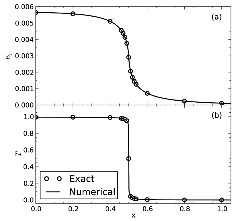
Figure 1.— Linear multigroup diffusion test. Numerical results are shown in lines, whereas the analytic solutions are shown in circle symbols. We show dimensionless total radiation energy density and temperature at the dimensionless time of 1 in panels (a) and (b), respectively. The spatial coordinate $x$ is also dimensionless.

Table 1Relative errors of linear multigroup diffusion test problem. The relative errors of temperature and total radiation energy density at the dimensionless time of 1 are shown.

$x$	$\epsilon(T)\times 10^{3}$	$\epsilon(E_{r})\times 10^{3}$	$x$	$\epsilon(T)\times 10^{3}$	$\epsilon(E_{r})\times 10^{3}$
0.00	0.0017	0.3209	0.51	4.8283	0.2585
0.20	0.0016	0.3220	0.52	1.8030	0.0232
0.40	0.0007	0.3460	0.53	1.0335	0.1495
0.46	0.0077	0.4095	0.54	0.7124	0.2330
0.47	0.0170	0.4443	0.60	0.3104	0.5469
0.48	0.0461	0.5136	0.80	0.5774	1.4067
0.49	0.2195	0.7169	1.00	1.3612	2.2413
0.50	0.0020	0.3712

The test we have simulated is the first problem in Shestakov & Bolstad (2005). We have set up the test using physical units rather than the dimensionless units of Shestakov & Offner (2008). The one-dimensional computational domain in physical units is $(0,1.0285926\times 10^{6})\,\mathrm{cm}$, corresponding to $(0,5.12)$ in dimensionless units. We use a symmetry boundary condition at the lower boundary, and a Marshak boundary with no incoming flux at the upper boundary (i.e., $E_{g}+(2/3\kappa_{g})\partial E_{g}/\partial x=0$). The mass density is $1.8212111\times 10^{-5}\,\mathrm{g}\,\mathrm{cm}^{-3}$. The specific heat capacity of the matter at constant volume is $9.9968637\times 10^{7}\,\mathrm{erg}\,\mathrm{K}^{-1}\mathrm{g}^{-1}$. Initially, the temperature is set to $0.1\,\mathrm{keV}$ and $0$, for ${x}<0.5$ and ${x}>0.5$, respectively. Here, ${x}$ is a dimensionless coordinate. The radiation energy density is initially set to zero everywhere. The constant $C_{\kappa}$ is set to $4.0628337\times 10^{43}\,\mathrm{cm}^{-1}\mathrm{Hz}^{3}$. The fixed temperature in the group-integrated radiation emission (Equation 98) is $T_{\mathrm{f}}=0.01\,\mathrm{keV}$, corresponding to $T_{\mathrm{f}}=0.1$ in dimensionless units. We use 64 radiation groups with the lowest boundary at zero. The width of the first group is set to $1.2089946\times 10^{13}\,\mathrm{Hz}$, corresponding to $5\times 10^{-4}$ in dimensionless units, and the width of other groups is set to be 1.1 times the width of its immediately preceding group. The representative frequency for each group is set to $\nu_{g}=\sqrt{\nu_{g-1/2}\,\nu_{g+1/2}}$, except that $\nu_{1}$ is set to $0.5\,\nu_{3/2}$ for the first group. We have run a simulation with 2048 uniform cells. Thus the dimensionless cell size is $1/400$. The time step is fixed at $5.8034112\times 10^{-8}\,\mathrm{s}$, corresponding to $1/200$ in dimensionless units. No acceleration scheme is used in this test. Figure 1 shows the results after 200 steps. The comparison with the tabular data of Shestakov & Offner (2008) is shown in Table 1. Relative errors are computed as $\epsilon(f)=|f_{\mathrm{n}}-f_{\mathrm{e}}|/f_{\mathrm{e}}$, where $f_{\mathrm{n}}$ and $f_{\mathrm{e}}$ are the numerical and exact results, respectively. Because the tabular data of the exact solution are located on the faces of numerical cells, averaging of the numerical data has been performed for the comparison. The results are in excellent agreement with the exact solution, and are comparable to the numerical results of Shestakov & Offner (2008).

Table 2$L_{1}$-norm errors and convergence rate for the total radiation energy density at the dimensionless time of 1 in the linear multigroup diffusion test problem. Four one-dimensional uniform-grid runs with various resolutions are shown. The errors are computed on the dimensionless domain of $(0,1)$.

$\Delta x$	$\Delta t$	$L_{1}$ Error	Convergence Rate
1/100	2/25	2.91E-3
1/200	1/50	7.36E-4	2.0
1/400	1/200	1.90E-4	1.9
1/800	1/800	4.87E-5	2.0

Table 3$L_{1}$-norm errors and convergence rate for the total radiation energy density at the dimensionless time of 1 in the linear multigroup diffusion test problem. Four one-dimensional AMR runs with various resolutions are shown. The errors are computed on the dimensionless domain of $(0,1)$.

$\Delta x$	$\Delta t$	$L_{1}$ Error	Convergence Rate
1/50, 1/100	4/25, 2/25	3.58E-3
1/100, 1/200	1/25, 1/50	1.05E-3	1.8
1/200, 1/400	1/100, 1/200	2.69E-4	2.0
1/400, 1/800	1/400, 1/800	6.82E-5	2.0

To assess the convergence behavior of our implicit scheme, we have performed a series of uniform-grid and AMR simulations of the linear multigroup diffusion test problem with various resolutions. The initial setup is the same as above except for spatial resolution and time step. Two levels are used in the AMR runs with the dimensionless domain of (0.25,0.75) covered by the fine (i.e., level 1) grids. In the convergence study, when the spatial resolution changes by a factor of 2 from one run to another, we change the time step by a factor of 4. Because our implicit scheme is first-order in time and second-order in space, the expected convergence rate in the convergence study is second-order with respect to $\Delta x$. Tables (2) and (3) show the $L_{1}$-norm errors and convergence rate for the total radiation energy density on the dimensionless spatial domain of $(0,1)$ at the dimensionless time of 1. Here, the $L_{1}$-norm error of the total radiation energy density is computed as

$$\epsilon_{1}(E_{r})=\frac{\sum_{i}|E_{r,i}-E_{r}(x_{i})|\Delta x_{i}}{\sum_{i}E_{r}(x_{i})\Delta x_{i}},$$ (99)

where $E_{r,i}=\sum_{g}E_{g,i}$ is the numerical result for cell $i$ and $E_{r}(x_{i})$ is the “exact” solution obtained from a high-resolution uniform-grid simulation with $\Delta x=1/3200$ and $\Delta t=1/12800$. The results of both uniform-grid and AMR simulations demonstrate second-order convergence rate with respect to $\Delta x$ as expected. Because only part of the domain in the AMR runs is covered by fine grids, the AMR runs have somewhat larger errors than the uniform-grid runs with the same resolution as the fine grids.

4.1.2 Nonequilibrium Radiative Transfer With Picket-Fence Model

Su & Olson (1999) have studied a nonequilibrium radiative transfer problem with a multigroup model, more specifically the picket-fence model. There are some special assumptions in this test problem. The volumetric heat capacity at constant volume is assumed to be $c_{v}=\alpha T^{3}$, where $T$ is the matter temperature and $\alpha$ is a parameter. The group-integrated Planck function is assumed to be

$$B_{g}=p_{g}\left(\frac{ac}{4\pi}\right)T^{4},$$ (100)

where $a$ is the radiation constant, and $p_{g}$ are parameters such that $\sum_{g}p_{g}=1$. It is also assumed that the absorption coefficient is independent of temperature and there is no scattering. Su & Olson (1999) have also defined dimensionless variables for convenience. The dimensionless spatial coordinate is defined as

$$x=\bar{\kappa}z,$$ (101)

where $z$ is the coordinate in physical units, and

$$\bar{\kappa}=\sum_{g}p_{g}\kappa_{g}.$$ (102)

The dimensionless time is defined as

$$\tau=\left(\frac{4ac\bar{\kappa}}{\alpha}\right)t,$$ (103)

where $t$ is the time in physical units. The dimensionless variables $U_{g}$ for radiation energy density and $V$ for matter energy density are defined as

$$U_{g} = \frac{E_{g}}{aT_{0}^{4}},$$ (104)

$$V = \left(\frac{T}{T_{0}}\right)^{4},$$ (105)

where $T_{0}$ is a reference temperature. In this test problem, there is a constant radiation source that exists for a finite period of time $(0\leq\tau\leq\tau_{0})$ on a finite range $(|x|<x_{0})$. Su & Olson (1999) have found analytic solutions to the problem for both transport and diffusion approaches.

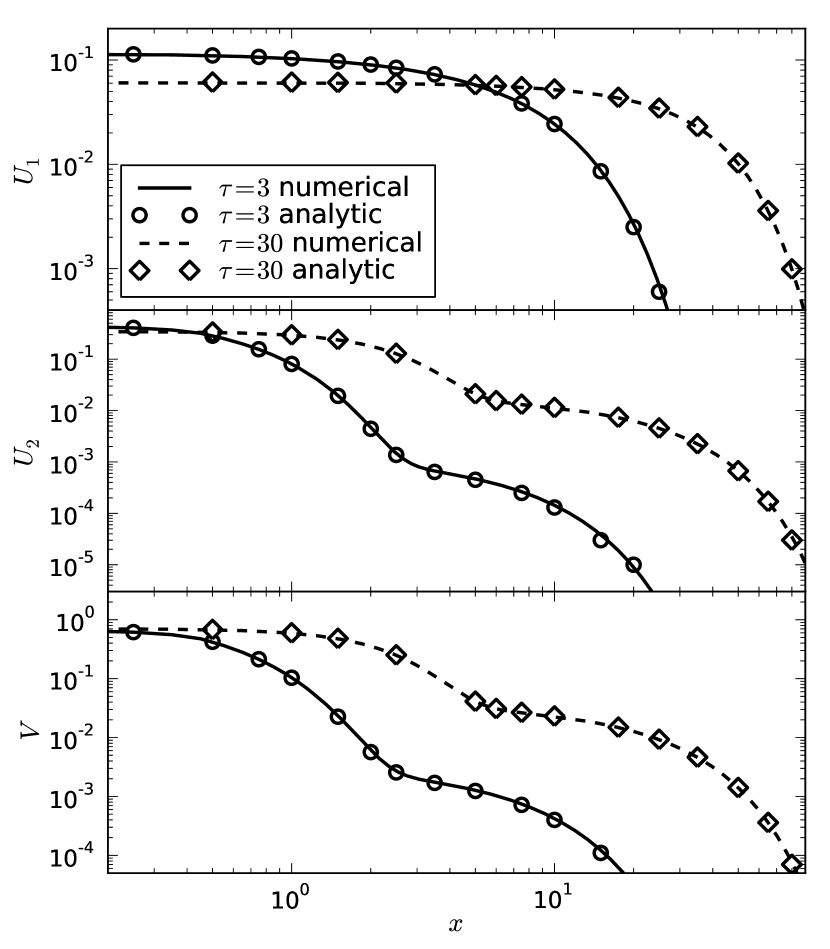
Figure 2.— Nonequilibrium radiative transfer with picket-fence model. Numerical results of $U_{1}$, $U_{2}$, and $V$ are shown for $\tau=3$ (solid lines) and $30$ (dashed lines). Also shown are analytic results for $\tau=3$ (circles) and $30$ (diamonds).

Here, we simulate the Case C of Su & Olson (1999) by solving the multigroup diffusion equations (Equations 95 & 96), and compare the results with the diffusion solution of Su & Olson (1999). Two radiation groups are used in this test, with $p_{1}=p_{2}=0.5$. The absorption coefficients are set to $\kappa_{1}=2/101\,\mathrm{cm}^{-1}$ and $\kappa_{2}=200/101\,\mathrm{cm}^{-1}$. Thus, $\bar{\kappa}=1\,\mathrm{cm}^{-1}$. The constant $\alpha$ in the expression for volumetric heat capacity is set to $\alpha=4a$. The reference temperature is chosen as $T_{0}=10^{6}\,\mathrm{K}$. The parameters for the radiation source are $x_{0}=0.5$, and $\tau_{0}=10$. When $\tau<\tau_{0}$, the radiation source deposits radiation energy to the region $|x|<x_{0}$ and increases the radiation energy density at a rate of $p_{g}c\bar{\kappa}aT_{0}^{4}$ for each group. The computational domain is $0<x<102.4$ covered by 1024 uniform cells. The lower boundary is symmetric, and the radiation energy density outside the upper boundary is set to zero. Initially, there is no radiation and the temperature is zero. A fixed time step $\Delta\tau=0.1$ is employed. The explicit solver is turned off in the simulation, and the radiation flux is not limited. No acceleration scheme is used in this test. The numerical results are shown in Figure 2. Our results are in excellent agreement with the analytic solution.

4.1.3 Radiating Sphere

Graziani (2008) found an analytic solution for the spectrum of a radiating sphere in a medium with frequency-dependent opacity. This test was used by Swesty & Myra (2009) to test their V2D code. In this test, a hot sphere with a fixed temperature is surrounded by a cold static medium. The absorption coefficient is assumed to be zero, and the radiative transfer is due to coherent and isotropic scattering. Thus, there is no radiation-matter coupling or group coupling. The time-dependent spectrum at a given place in the medium is therefore the superposition of the black-body spectrum of the medium and the spectrum of the radiation originated from the hot sphere.

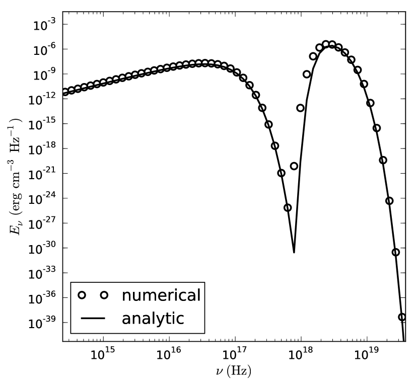
Figure 3.— Spectrum from the radiating sphere observed at $t=10^{-12}\,\mathrm{cm}$ and $r=0.06\,\mathrm{cm}$. Both numerical (circle symbols) and analytic (solid line) results are shown.

We perform this test in one-dimensional spherical geometry. The computational domain is $0.02\,\mathrm{cm}<r<0.1\,\mathrm{cm}$ and is covered by 128 uniform cells. The hot sphere has a fixed temperature of $1.5\,\mathrm{keV}$, and the medium is at $50\,\mathrm{eV}$. We use 60 energy groups covering an energy range of $0.5\,\mathrm{eV}$ to $308\,\mathrm{keV}$. The group Rosseland mean coefficient is assumed to be $\chi_{g}=10^{13}(\nu_{g}/3.6\times 10^{14}\,\mathrm{Hz})^{-3}\,\mathrm{cm}^{-1}$. The explicit solver is turned off. No acceleration scheme is used in this test. There is no outer iteration in the implicit solver because the matter properties do not change. The time step is fixed at $10^{-15}\,\mathrm{s}$. The spectrum at $r=0.06\,\mathrm{cm}$ and $t=10^{-12}\,\mathrm{s}$ is shown in Figure 3. The numerical results are again in good agreement with the analytic solution.

4.1.4 Shock Tube Problem In Strong Equilibrium Regime

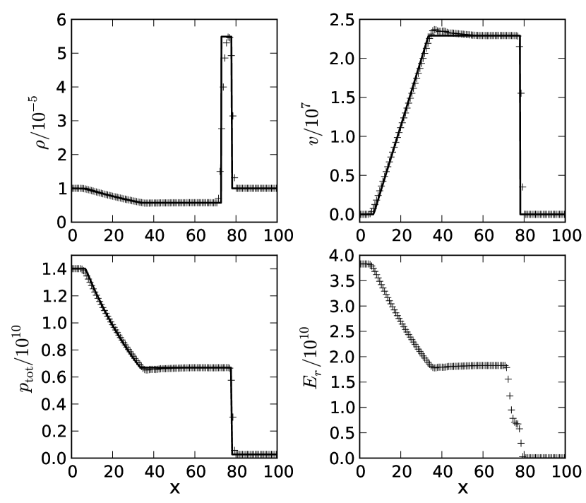
Figure 4.— Shock tube at $t=10^{-6}\,\mathrm{s}$. Numerical results from a full radiation hydrodynamics calculation with 16 radiation groups and 128 cells are shown in symbols. The exact solutions of a pure hydrodynamic Riemann problem corresponding to the numerical problem are shown in solid lines for comparison. We show mass density ($\rho$), velocity ($v$), total pressure ($p_{\mathrm{tot}}$), and radiation energy density ($E_{r}$). For the radiation hydrodynamics simulation, the total pressure is the sum of gas pressure and radiation pressure, and the radiation energy density is summed over all groups. In the pure hydrodynamic Riemann problem, there is no radiation energy density. All quantities are in cgs units.

In this one-dimensional problem, the initial conditions of the matter are $\rho_{L}=10^{-5}\,\mathrm{g}\,\mathrm{cm}^{-3}$, $T_{L}=1.5\times 10^{6}\,\mathrm{K}$, $u_{L}=0$ and $\rho_{R}=10^{-5}\,\mathrm{g}\,\mathrm{cm}^{-3}$, $T_{R}=3\times 10^{5}\,\mathrm{K}$, $u_{R}=0$, where $L$ stands for the left half, and $R$ the right half of the computational domain ($0<x<100\,\mathrm{cm}$). The gas is assumed to be ideal with an adiabatic index of $\gamma=4/3$ and a mean molecular weight of $\mu=1$. Initially, the radiation is assumed to be in thermal equilibrium with the gas (i.e., $E_{g}=4\pi B_{g}/c$). The interaction coefficients are set to $\kappa_{g}=10^{6}\,\mathrm{cm}^{-1}$ and $\chi_{\mathrm{g}}=10^{8}\,\mathrm{cm}^{-1}$. Thus, due to the huge opacities, the system is close to the limit of strong equilibrium with no diffusion, and is essentially governed by Equations (30)–(34) with $\lambda_{g}=1/3$ and $f_{g}=1/3$. The parameters of this test problem are chosen such that neither radiation pressure nor gas pressure can be ignored. This test is adapted from the shock tube problem in Paper II. However, the adiabatic index of the gas is now $\gamma=4/3$ rather than $5/3$ so that we can compare the numerical results with the exact solution of a pure hydrodynamic Riemann problem. Furthermore, although this is a one-temperature gray problem due to the huge opacity, the numerical calculation is performed with 16 radiation groups with the lowest and uppermost boundaries at $10^{14}\,\mathrm{Hz}$ and $10^{18}\,\mathrm{Hz}$, respectively. We use 128 uniform zones in this test. The numerical results are shown in Figure 4. Also shown are the exact solutions of a pure hydrodynamic Riemann problem corresponding to the numerical problem. The results show good agreement. We also note that our scheme is stable without using small time steps even though the system is in the “dynamic diffusion” limit (Mihalas & Mihalas, 1999) with $\tau u/c\sim 10^{7}$, where $\tau$ is the optical depth of the system. Either the gray acceleration scheme or the local acceleration scheme (§ 3.2.4) must be employed in this test, otherwise the implicit solver, which is responsible for the thermal equilibrium between radiation and matter, exhibits extremely slow convergence.

4.1.5 Nonequilibrium Radiative Shock

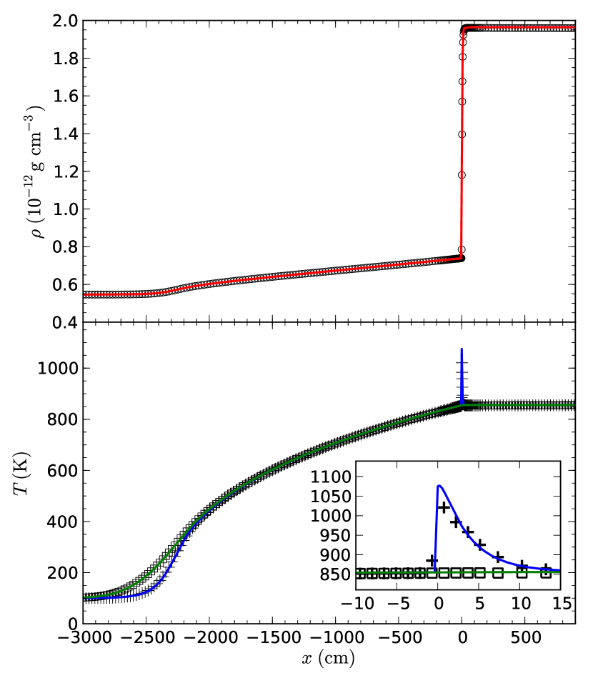
Figure 5.— Density and temperature profiles for Mach 5 supercritical shock. Numerical results are shown in symbols. We show density (circles), gas temperature (plus signs), and radiation temperature (squares). Here radiation temperature is defined as $(E_{r}/a)^{1/4}$, where $E_{r}$ is the total radiation energy density. Also shown are the analytic results for density (red solid line), gas temperature (blue solid line), and radiation temperature (green solid line). We show only part of the region near the density jump. The inset shows a blow-up of the spike in temperature. The numerical results have been shifted by $-207\,\mathrm{cm}$ in space to compensate for the discrepancy in shock position caused by the initial setup.

In this test, we simulate the Mach 5 shock problem of Lowrie & Edwards (2008). In Paper II, we showed results computed with the gray radiation hydrodynamics solver. Here, we present the numerical results obtained with the multigroup radiation hydrodynamics solver. In this test, the one-dimensional numerical region $(-4000\,\mathrm{cm},2000\,\mathrm{cm})$ initially consists of two constant states: $\rho_{L}=5.45969\times 10^{-13}\,\mathrm{g}\,\mathrm{cm}^{-3}$, $T_{L}=100\,\mathrm{K}$, $u_{L}=5.88588\times 10^{5}\,\mathrm{cm}\,\mathrm{s}^{-1}$ and $\rho_{R}=1.96435\times 10^{-12}\,\mathrm{g}\,\mathrm{cm}^{-3}$, $T_{R}=855.720\,\mathrm{K}$, $u_{R}=1.63592\times 10^{5}\,\mathrm{cm}\,\mathrm{s}^{-1}$, where $L$ stands for the left, and $R$ the right of the point $x=0$, respectively. The gas is assumed to be ideal with an adiabatic index of $\gamma=5/3$ and a mean molecular weight of $\mu=1$. The setup is the same as that in Paper II except that 16 radiation groups are used in this paper. The lowest and uppermost boundaries of the groups are at $10^{10}\,\mathrm{Hz}$, and $10^{15}\,\mathrm{Hz}$, respectively. Initially, the radiation is assumed to be in thermal equilibrium with the gas (i.e., $E_{g}=4\pi B_{g}/c$). The interaction coefficients are set to $\kappa_{g}=3.92664\times 10^{-5}\,\mathrm{cm}^{-1}$ and $\chi_{g}=0.848903\,\mathrm{cm}^{-1}$, respectively. The states at spatial boundaries are held at fixed values. Four refinement levels (five total levels) are used with a refinement factor of 2 with the finest resolution being $\Delta x\approx 1.5\,\mathrm{cm}$. In this test, a cell is tagged for refinement if the second derivative of either density or temperature exceeds certain thresholds (Paper II). The initial conditions are set according to the pre-shock and post-shock states of the Mach 5 shock. After a brief period of adjustment, the system settles down to a steady shock. The simulation is stopped at $t=0.04\,\mathrm{s}$. The results are shown in Figure 5. The agreement with the analytic solution including the narrow spike in temperature is excellent, except that the numerical results in the figure had to be shifted by $-207\,\mathrm{cm}$ in space to match the analytic shock position. This discrepancy in shock position is due to the initial transient phase as the initial state relaxes to the correct steady-state profile. No flux limiter is used in this calculation because the analytic solution of Lowrie & Edwards (2008) assumes $\lambda=1/3$. We again found that the implicit solver would fail to converge without an acceleration scheme. Both the gray acceleration scheme and the local acceleration scheme (§ 3.2.4) work in this test.

4.1.6 Advecting Radiation Pulse

In Paper II, we performed a test of advecting a radiation pulse by the motion of matter with the gray radiation hydrodynamics solver (see also Krumholz et al., 2007). Here, we repeat the test with small changes to exercise the multigroup aspect of CASTRO. The setup is the same as that in Paper II, except that the absorption coefficient $\kappa$ in this paper is given by

$$\kappa=180\left(\frac{T}{10^{7}\,\mathrm{K}}\right)^{-0.5}\left(\frac{\nu}{10^{18}\,\mathrm{Hz}}\right)^{-3}\left[1-\exp\left(-\frac{h\nu}{kT}\right)\right]\,\mathrm{cm}^{-1}.$$ (106)

As in the test in Paper II, the initial temperature and density profiles are

$$T = T_{0}+(T_{1}-T_{0})\exp{\left(-\frac{x^{2}}{2w^{2}}\right)},$$ (107)

$$\rho = \rho_{0}\frac{T_{0}}{T_{1}}+\frac{a\mu}{3R}\left(\frac{T_{0}^{4}}{T}-T^{3}\right),$$ (108)

where $T_{0}=10^{7}\,\mathrm{K}$, $T_{1}=2\times 10^{7}\,\mathrm{K}$, $\rho_{0}=1.2\,\mathrm{g\>cm}^{-3}$, $w=24\,\mathrm{cm}$, the mean molecular weight of the gas is $\mu=2.33$, and $R$ is the ideal gas constant. Initially the radiation is assumed to be in thermal equilibrium with the gas. No flux limiter is used in this test (i.e., $\lambda=1/3$ and $f=1/3$). If there were no radiation diffusion, the system would be in an equilibrium with the gas pressure and radiation pressure balancing each other. Because of radiation diffusion, the balance is lost and the gas moves.

The purpose of this test is twofold. First, we use this test to assess the ability of the code to handle radiation being advected by the motion of matter. We solve the problem numerically in different laboratory frames. Then we compare the case in which the gas is initially at rest to the case in which the gas initially moves at a constant velocity. Another purpose is to assess the effect of group resolution. Since the opacity is very large, the system is close to thermal equilibrium between radiation and matter. Hence, the results of multigroup radiation hydrodynamics simulations should become increasingly close to those of a gray radiation hydrodynamics simulation as more groups are used.

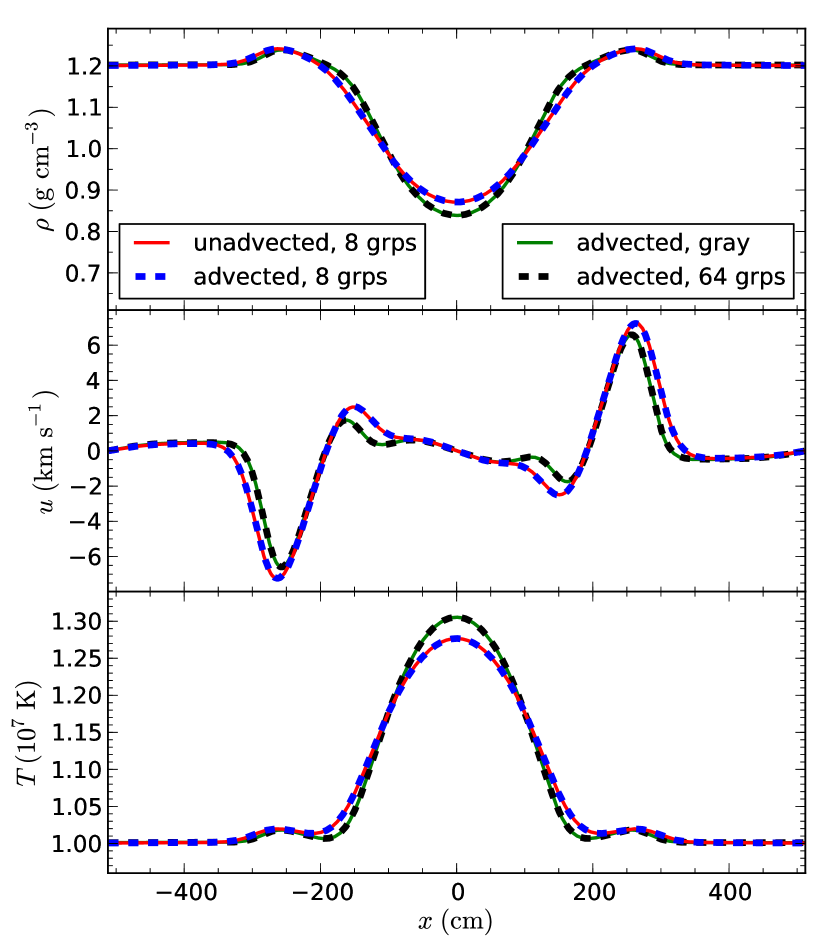
Figure 6.— Density, velocity and temperature profiles at $t=4.8\times 10^{-5}\,\mathrm{s}$ for the test of advecting radiation pulse. We show the results of four runs including the unadvected 8-group run (red solid lines), the advected 8-group run (blue dotted lines), the advected 64-group run (black dotted lines), and the advected gray run (green solid lines). The results of the advected runs have been shifted in space for comparison.

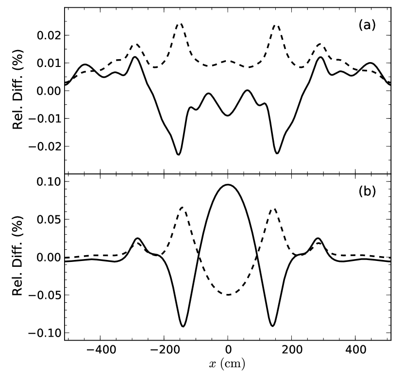
Figure 7.— Relative differences in density (solid lines) and gas temperature (dashed lines) in the test of advecting radiation pulse. The relative differences between the advected 8-group and unadvected 8-group runs are shown in panel (a), whereas the relative differences between the advected 64-group and advected gray runs in panel (b).

We have performed four runs: an unadvected run with 8 radiation groups, an advected run with 8 groups, an advected run with 64 groups, and an advected run using the gray radiation hydrodynamics solver presented in Paper II. The velocity in the unadvected run is initially zero everywhere, whereas in the advected runs it is $10^{6}\,\mathrm{cm\>s}^{-1}$ everywhere. For the multigroup runs, the lowest and uppermost group boundaries are at $10^{15}\,\mathrm{Hz}$ and $10^{19}\,\mathrm{Hz}$, respectively. In the gray simulation, the single group Planck mean coefficient, $\kappa_{\mathrm{P}}$, and Rosseland mean coefficient, $\kappa_{\mathrm{R}}$, of the opacity given by Equation (106) are

$$\kappa_{\mathrm{P}} = 3063.96\left(\frac{T}{10^{7}\,\mathrm{K}}\right)^{-3.5}\,\mathrm{cm}^{-1},$$ (109)

$$\kappa_{\mathrm{R}} = 101.248\left(\frac{T}{10^{7}\,\mathrm{K}}\right)^{-3.5}\,\mathrm{cm}^{-1}.$$ (110)

The computational domain in all four runs is a one-dimensional region of $-512\,\mathrm{cm}<x<512\,\mathrm{cm}$ with periodic boundaries. The numerical grid consists of 512 uniform cells. The simulations are stopped at $t=4.8\times 10^{-5}\,\mathrm{s}$. Figure 6 shows the density, velocity, and temperature profiles for all four runs. The results of the advected runs have been shifted in space for comparison. The profiles from the unadvected 8-group run and the advected 8-group run are almost identical demonstrating the accuracy of our scheme in handling radiation advection by the motion of matter. This is expected because the velocity is significantly smaller than the speed of light ($v/c\sim 3\times 10^{-5}$). The results from the advected 64-group run and the gray run are also almost identical as expected. It is clear that the 8-group results differ from the gray results. This is not surprising because we did not perform group averaging for interaction coefficients (Equations 21 & 22). We also show the relative differences in Figure 7. The relative difference of the advected 8-group run with respect to the unadvected 8-group run is computed as (advected - unadvected) / unadvected, and the relative difference of the 64-group run with respect to the gray run is computed as (multigroup - gray) / gray. The figure shows that the difference between the advected 8-group and unadvected 8-group runs is less than 0.03% everywhere, and the difference between the 64-group and gray runs is less than 0.1% everywhere.

4.1.7 Static Equilibrium

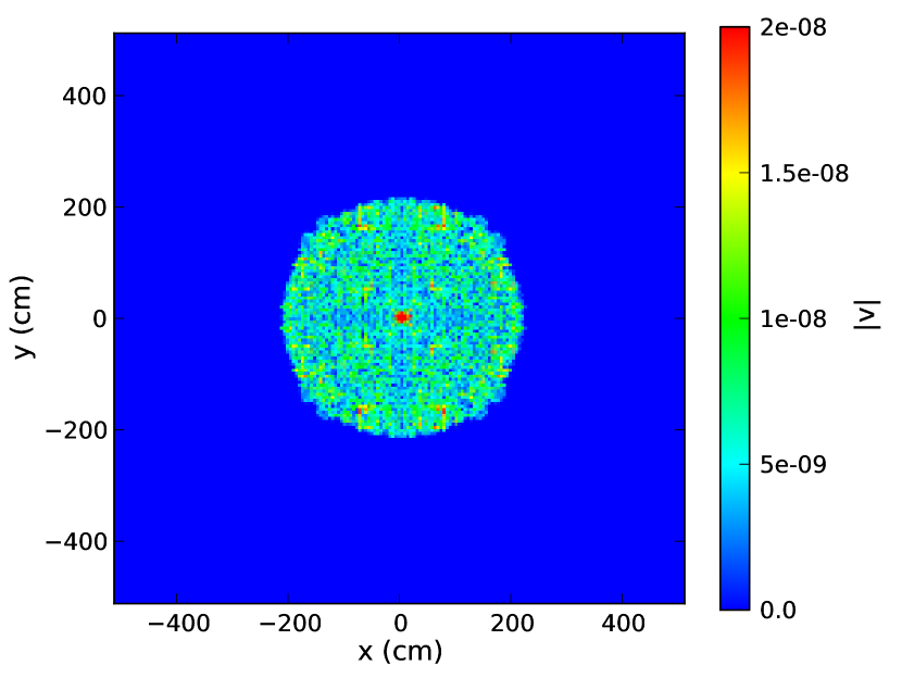
Figure 8.— Structure of the magnitude of velocity at $t=10^{-4}\,\mathrm{s}$ in the static equilibrium test. The unit of velocity is $\mathrm{cm\>s}^{-1}$.

In Paper II, we have demonstrated that the gray solver can maintain a perfect static equilibrium in multiple dimensions because the radiation pressure and the gas pressure are coupled in the Riemann solver. Here, we repeat the test using the multigroup solver. The setup is the same as that in Paper II. The initial conditions for radiation and matter are the same as those in the test of the advecting radiation pulse (§ 4.1.6) except that the interaction coefficients are set to a very high value, $\kappa_{g}=\chi_{g}=10^{20}\,\mathrm{cm}^{2}\,\mathrm{g}^{-1}\times\rho$. Thus, almost no diffusion can happen, and the radiation and the matter are in perfect thermal equilibrium. We have performed a calculation on a two-dimensional Cartesian grid of $-512\,\mathrm{cm}<x<512\,\mathrm{cm}$ and $-512\,\mathrm{cm}<y<512\,\mathrm{cm}$ with 512 uniform cells in each direction. The initial velocity is zero everywhere. For the initial setup, the coordinate $x$ in equation (107) is replaced by $r=\sqrt{x^{2}+y^{2}}$. We use 16 radiation groups with the lowest and uppermost boundaries at $10^{15}\,\mathrm{Hz}$ and $10^{19}\,\mathrm{Hz}$, respectively. Figure 8 shows the velocity profile at $t=10^{-4}\,\mathrm{s}$ (after about 6000 steps). The maximal velocity at that time is $\sim 8\times 10^{-8}\,\mathrm{cm\>s}^{-1}$, which is about $10^{-15}$ of the sound speed. Such a small gas velocity indicates that the multigroup solver in CASTRO can also maintain a perfect static equilibrium in multiple dimensions, as does the gray solver in CASTRO.

4.2. Core-Collapse Supernova Simulations

In this section, we present core-collapse supernova simulations in 1D spherical and 2D cylindrical coordinates. Newtonian gravity with a monopole approximation is used in the 2D simulation for simplicity, although CASTRO has a multigrid Poisson solver for gravity. In the simulations, there are three neutrino species: electron neutrinos, $\nu_{e}$, electron antineutrinos, $\bar{\nu}_{e}$, and $\nu_{\mu}$ which stands for a combined species representing $\nu_{\mu}$, $\nu_{\tau}$, $\bar{\nu}_{\mu}$, and $\bar{\nu}_{\tau}$. We use a tabular equation of state that provides thermodynamic quantities as a function of temperature, density, and electron fraction and was constructed from the Shen et al. (1998a, b) mean-field table, augmented with photons and a general electron/positron equation of state, and extended down to $10\>\mathrm{g}\>\mathrm{cm}^{-3}$. The opacities used are fully described in Burrows et al. (2006). They include 1) elastic scattering off nucleons, alpha particles, and the single representative heavy nucleus at the peak of the binding energy curve calculated by Shen et al. (1998a, b), and 2) charged-current absorption cross sections off nucleons and nuclei (the latter using the approach of Bruenn (1985)). The scattering and absorption cross sections off nucleons are corrected for weak magnetism and recoil effects, the form factor, electron screening, and ion-ion correlation effects on Freedman scattering off nuclei are applied, and pair production by nucleon-nucleon bremsstrahlung and electron-positron annihilation (and their inverses) are included as sources (and sinks). The sink terms of the latter do not include Fermi blocking corrections by the neutrinos in the final state. Inelastic neutrino-electron scattering is treated as elastic scattering.

4.2.1 One-Dimensional Core-Collapse Supernova Simulation

We present here a core-collapse supernova simulation in one-dimensional spherical coordinates. The initial model is based on a $15\,M_{\odot}$ progenitor of Woosley & Weaver (1995). The computational domain for this run is $0<r<5\times 10^{8}\,\mathrm{cm}$. The simulation employs four refinement levels (five total levels) with 1024 zones on the coarsest level (i.e., level 0) and a resolution of $\Delta r\approx 0.305\,\mathrm{km}$ on the finest level (i.e., level 4). The AMR refinement factor is 2. The regions where the density is greater than $7.2\times 10^{6}\,\mathrm{g}\,\mathrm{cm}^{-3}$, or the enclosed mass is greater than $1.32\,M_{\odot}$ are refined to level 2. In addition, cells on level $\ell$ will be refined to level $\ell+1$ if $Y_{e}<0.4$, $s>5$, $\nabla Y_{e}>0.01/\Delta r_{\ell}$, or $\nabla s>1/\Delta r_{\ell}$, where $\ell<4$, $s$ is entropy in units of $k\,\mathrm{baryon}^{-1}$, and $\Delta r_{\ell}$ is the cell width on level $\ell$. We use 40 energy groups for electron neutrinos with the first group at $1\,\mathrm{MeV}$ and the last group at $300\,\mathrm{MeV}$. We use 32 energy groups for electron antineutrinos with the first and last groups at $1\,\mathrm{MeV}$ and $100\,\mathrm{MeV}$, respectively. For $\nu_{\mu}$, we use 40 energy groups with the first and last groups at $1\,\mathrm{MeV}$ and $300\,\mathrm{MeV}$, respectively. The flux limiter of Levermore & Pomraning (1981) is used is this simulation. The local acceleration scheme is employed. The inner boundary is symmetric. An outflow boundary condition is used for the outer boundary in the explicit solver. The modified Marshak boundary of Sanchez & Pomraning (1991) with zero incoming flux is used for the outer boundary in the implicit solver. Thus, the region outside the outer boundary is essentially treated as a vacuum, and the radiation diffuses into the vacuum. Note that in the usual Marshak boundary based on the classical diffusion theory, the flux at the boundary does not have the correct behavior in the streaming limit, and the issue has been fixed in the modified Marshak boundary of Sanchez & Pomraning (1991) by using flux limited diffusion.

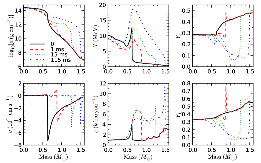
Figure 9.— Density (upper left), velocity (lower left), temperature (upper center), entropy per baryon (lower center), electron fraction (upper right), and net lepton fraction (lower right) as a function of enclosed mass for the 1D core-collapse supernova simulation. Snapshots are shown for 0 (black solid lines), 1 ms (red dashed lines), 15 ms (green dotted lines), and 115 ms (blue dash-dotted lines) after bounce.

The simulation is carried out to 200 ms after core bounce. Figure 9 shows four snapshots of density, velocity, temperature, entropy, electron fraction, and net electron lepton fraction ($Y_{L}$). The infall of the material due to gravity results in the increase of the central density until the core bounces. At bounce, the density reaches $\rho^{\mathrm{core}}\approx 2.9\times 10^{14}\>\mathrm{g}\>\mathrm{cm}^{-3}$ at the core. A shock appears around bounce at $M_{\mathrm{sh}}\approx 0.635M_{\odot}$. The electron and lepton fractions at bounce are $Y_{e}^{\mathrm{core}}\approx 0.288$ and $Y_{L}^{\mathrm{core}}\approx 0.326$, respectively, at the core. The core temperature at bounce is $T^{\mathrm{core}}\approx 9.98\>\mathrm{MeV}$. The core entropy at bounce is $s^{\mathrm{core}}\approx 0.901\>k\>\mathrm{baryon}^{-1}$. These properties are in agreement with previous studies (e.g., Rampp & Janka, 2000; Liebendörfer et al., 2001; Thompson et al., 2003). In a recent study, Lentz et al. (2012) have obtained $M_{\mathrm{sh}}\approx 0.492\>\mathrm{M_{\odot}}$, $\rho_{\mathrm{core}}\approx 4.264\times 10^{14}\>\mathrm{g}\>\mathrm{cm}^{-3}$, $Y_{e}^{\mathrm{core}}\approx 0.2407$, and $Y_{L}^{\mathrm{core}}\approx 0.2782$ for their model N-FullOp at bounce, and $M_{\mathrm{sh}}\approx 0.717\>\mathrm{M_{\odot}}$, $\rho_{\mathrm{core}}\approx 3.336\times 10^{14}\>\mathrm{g}\>\mathrm{cm}^{-3}$, $Y_{e}^{\mathrm{core}}\approx 0.3046$, and $Y_{L}^{\mathrm{core}}\approx 0.3696$ for their model N-ReduceOp at bounce. Except for $\rho_{\mathrm{core}}$, the properties of our model at bounce are in between those in models N-FullOp and N-ReduceOp of Lentz et al. (2012).

Figure 9 shows a spike near the shock in the $Y_{e}$ and $Y_{L}$ profiles shortly after bounce (see also Lentz et al., 2012). The spike of $Y_{L}$ is caused by electron neutrinos leaking out of the shock. The absorption of some of those neutrinos by the pre-shock material results in a spike of $Y_{e}$. In the post-shock region, the minimal $Y_{e}$ drops rapidly for the first few milliseconds after bounce due to electron capture; it then becomes steady at $\sim 0.065-0.075$. The velocity in some region behind the shock is positive for the first $\sim$ 2 ms after bounce; the maximum positive velocity reaches $\sim 2\times 10^{9}\>\mathrm{cm}\;\mathrm{s}^{-1}$ similar to the maximum positive velocity in Thompson et al. (2003). The maximum temperature in the shocked region increases rapidly to $17.5\>\mathrm{MeV}$ at $\sim 0.1\>\mathrm{ms}$ after bounce; it then decreases quickly as the shock expands outward in radius; it increases again and reaches $\sim 22\>\mathrm{MeV}$ at 200 ms after bounce due to compression and deleptonization as matter settles onto the proto-neutron star. The evolution of the temperature, electron fraction and velocity profiles is in agreement with that in previous studies (e.g., Thompson et al., 2003).

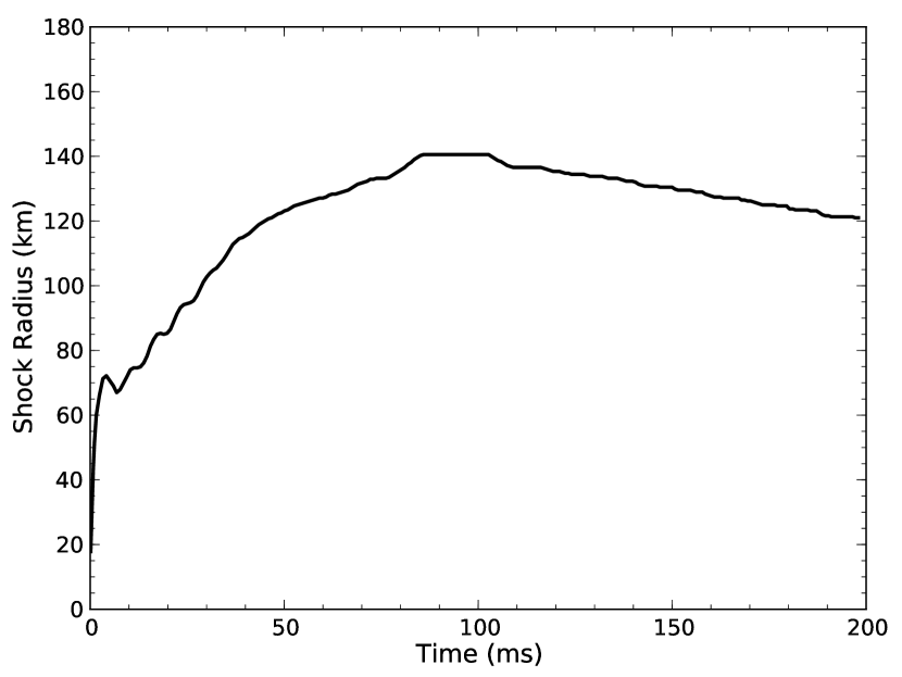
Figure 10.— Shock radius vs. post-bounce time for the 1D core-collapse supernova simulation. The shock position is defined as the place with the largest negative gradient of radial velocity. The peak shock radius reaches $\sim 140\>\mathrm{km}$ at $\sim 100\>\mathrm{ms}$ after bounce.

In Figure 10, we show shock radius as a function of time. For the first few milliseconds after bounce, the shock expands very rapidly in radius, and reaches $\sim 72\>\mathrm{km}$. The peak shock radius reaches $\sim 140\>\mathrm{km}$ at $\sim 100\>\mathrm{ms}$ after bounce. After that the shock slowly shrinks in radius although it continues to grow in mass.

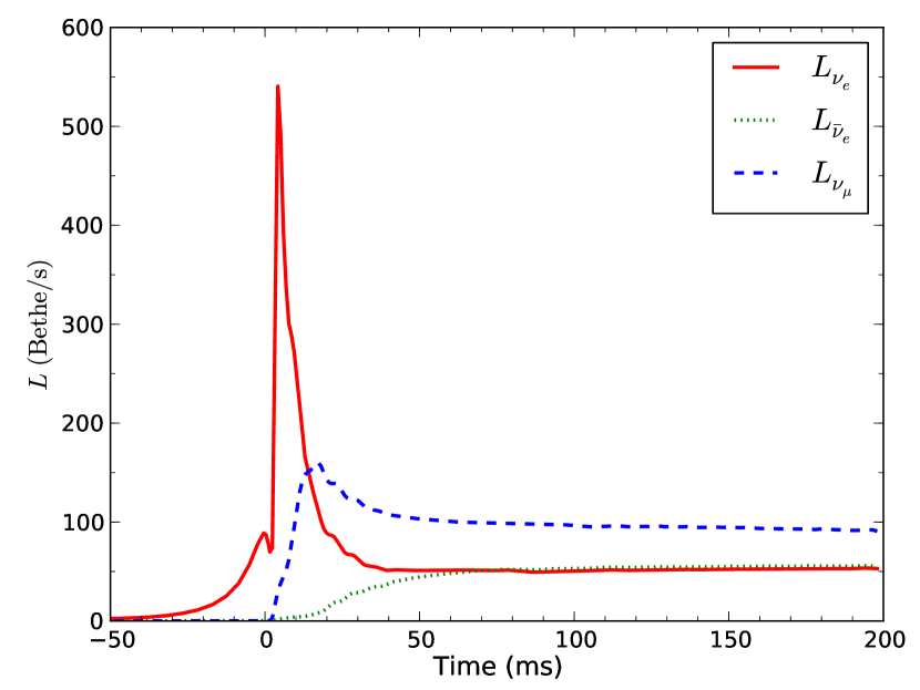
Figure 11.— Comoving frame luminosities of $\nu_{e}$ (red solid line), $\bar{\nu}_{e}$ (green dotted line), and $\nu_{\mu}$ neutrinos (blue dashed line) measured at 500 km for the 1D core-collapse supernova simulation. The luminosity of electron neutrinos reaches a peak value of $540\>\mathrm{Bethe}\>\mathrm{s}^{-1}$ at 4 ms after bounce. For $L_{\nu_{e}}$, the full width at half maximum is $\sim 7\>\mathrm{ms}$. There is also a noticeable spike in the luminosity of $\nu_{\mu}$ neutrinos with a peak value of $160\>\mathrm{Bethe}\>\mathrm{s}^{-1}$ at $17\>\mathrm{ms}$ after bounce.

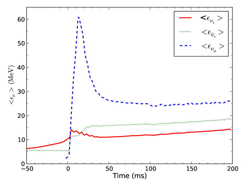
Figure 12.— Rms average energies of $\nu_{e}$ (red solid line), $\bar{\nu}_{e}$ (green dotted line), and $\nu_{\mu}$ neutrinos (blue dashed line) measured at 500 km for the 1D core-collapse supernova simulation. For $\langle\epsilon_{\nu_{\mu}}\rangle$, the peak value of $61\>\mathrm{MeV}$ is reached at 13 ms after bounce. The rms average energies at 200 ms after bounce are $14$, $19$, and $26\>\mathrm{MeV}$, for $\nu_{e}$, $\bar{\nu}_{e}$, and $\nu_{\mu}$, respectively. We do not show $\langle\epsilon_{\nu_{\mu}}\rangle$ before bounce because there is very little $\nu_{\mu}$ at those early times.

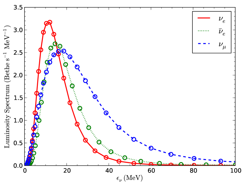
Figure 13.— Luminosity spectrum of $\nu_{e}$ (red solid line), $\bar{\nu}_{e}$ (green dotted line), and $\nu_{\mu}$ neutrinos (blue dashed line) measured at 500 km and 200 ms after bounce for the 1D core-collapse supernova simulation. The actual energy groups are shown in circles.

The comoving frame luminosities of $\nu_{e}$, $\bar{\nu}_{e}$, and $\nu_{\mu}$ neutrinos measured at 500 km are shown in Figure 11. In agreement with previous studies (e.g., Thompson et al., 2003; Marek & Janka, 2009; Lentz et al., 2012), there is a small dip in $L_{\nu_{e}}$ after the initial rise. The dip is followed by a large pulse in $L_{\nu_{e}}$ that reaches $540\>\mathrm{Bethe}\>\mathrm{s}^{-1}$ at 4 ms after bounce. The full width at half maximum for $L_{\nu_{e}}$ is $\sim 7\>\mathrm{ms}$. The peak $L_{\nu_{e}}$ in our model is about 20% larger than that in Marek & Janka (2009); Lentz et al. (2012). In our results, there is also a noticeable spike in $L_{\nu_{\mu}}$. Note that Thompson et al. (2003); Lentz et al. (2012) have obtained somewhat similar spikes in their simulations that did not include inelastic scattering. The lack of inelastic scattering of neutrinos on electrons results in harder neutrino spectra, especially for $\nu_{\mu}$, as shown in the rms average energies (Figure 12). Here the rms average is defined as

$$\langle\epsilon_{\nu}\rangle=\left[\frac{\int\epsilon_{\nu}^{2}n_{\nu}\mathrm{d}\nu}{\int n_{\nu}\mathrm{d}\nu}\right]^{1/2},$$ (111)

where $\epsilon_{\nu}$ is the neutrino energy and $n_{\nu}$ is the monochromatic neutrino number density. Nevertheless we obtain $\langle\epsilon_{\nu_{e}}\rangle<\langle\epsilon_{\bar{\nu}_{e}}\rangle<\langle\epsilon_{\nu_{\mu}}\rangle$ after the initial phases, as expected. At 200 ms after bounce, we obtain $\langle\epsilon_{\nu_{e}}\rangle\approx 14$, $\langle\epsilon_{\bar{\nu}_{e}}\rangle\approx 19$, and $\langle\epsilon_{\nu_{\mu}}\rangle\approx 26\>\mathrm{MeV}$. The luminosity spectra measured at 500 km in the comoving are shown Figure 13. The spectra are evidently harder than those in Thompson et al. (2003) because inelastic scattering is not included in our model.

4.2.2 Two-Dimensional Core-Collapse Supernova Simulation

Here we present a two-dimensional core-collapse supernova simulation. The computational domain for this 2D cylindrical run is $0<r<2.5\times 10^{8}\,\mathrm{cm}$ and $-2.5\times 10^{8}\,\mathrm{cm}<z<2.5\times 10^{8}\,\mathrm{cm}$. Two refinement levels (three total levels) with a refinement factor of 4 are used. The coarsest level has 256 and 512 cells at $r$-direction and $z$-direction, respectively. Thus the size of the cells on the finest level is about $0.61\,\mathrm{km}$. The same refinement criteria as those in the 1D simulation in Section 4.2.1 are used. We use 20, 16, and 20 groups with logarithmic spacing for $\nu_{e}$, $\bar{\nu}_{e}$, and $\nu_{\mu}$, respectively. The other aspects of this 2D run such as the outer boundary and flux limiter are the same as those in the 1D simulation in Section 4.2.1. We start the 2D simulation from the result of a 1D simulation rather than the $15\,M_{\odot}$ presupernova model. The initial model is obtained from the 1D simulation at about 10 ms before bounce. At that time, multi-dimensional effects are expected to still be small. The 1D simulation that provides the initial model for the 2D run has similar resolution as the 2D run. Note that, other than resolution, the low-resolution 1D simulation here is essentially the same as the 1D high-resolution simulation in Section 4.2.1.

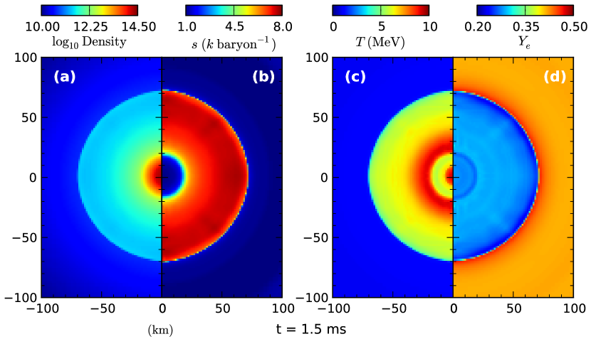
Figure 14.— Snapshot at 1.5 ms after bounce for the 2D cylindrical core-collapse supernova simulation. We show (a) logarithmic density, (b) entropy per baryon, (c) temperature, and (d) electron fraction, where the unit for density is $\mathrm{g}\>\mathrm{cm}^{-3}$. Only the inner 100 km of the model is shown here.

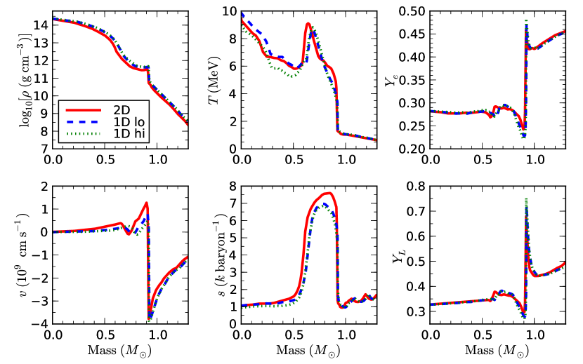
Figure 15.— Density (upper left), radial velocity (lower left), temperature (upper center), entropy per baryon (lower center), electron fraction (upper right), and net lepton fraction (lower right) as a function of enclosed mass at 1.5 ms after bounce. Here, radial velocity is the velocity in spherical radial direction. We show the results of the 2D cylindrical simulation (red solid lines), 1D low-resolution spherical run (blue dashed lines), and 1D high-resolution spherical run (green dotted lines). The radial profiles of the 2D results are generated via averaging.

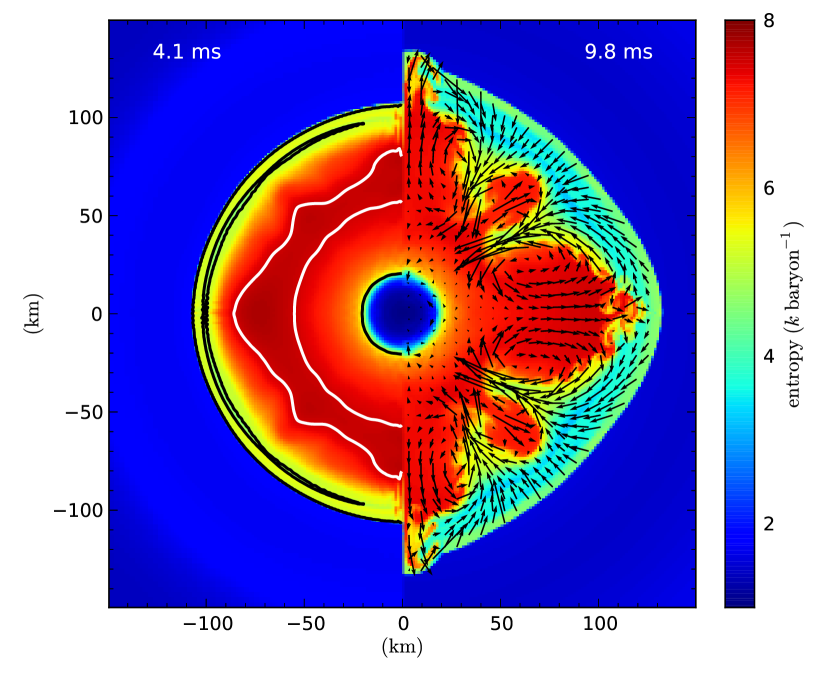
Figure 16.— Entropy at 4.1 (left) and 9.8 ms (right) after bounce for the 2D cylindrical core-collapse supernova simulation. The white and black contour lines in the left panel denote $s=7.5$ and $5\>k\>\mathrm{baryon}^{-1}$, respectively. The arrows in the right panel show the velocity field in the shocked region at 9.8 ms after bounce. It is shown that convection has developed in the shocked region at 9.8 ms after bounce.

Figure 14 shows the density, entropy, temperature, and electron fraction profiles at 1.5 ms after bounce. The profiles are still highly symmetric. Spherically averaged profiles of density, velocity, temperature, entropy, electron fraction, and lepton fraction at 1.5 ms are shown in Figure 15. Also shown in Figure 15 are the results of the two 1D runs. At this point, the 2D results are only slightly different from the 1D results. However, in some region behind the shock, the gradient of entropy is negative. A negative entropy gradient region from $\sim 70\,\mathrm{km}$ to $\sim 100\,\mathrm{km}$ is also clearly visible in the entropy profile at 4.1 ms (left panel of Figure 16). The white and black contour lines in the left panel of Figure 16 denote $s=7.5$ and $5\>k\>\mathrm{baryon}^{-1}$, respectively. Convective instabilities can potentially develop in the region between $\sim 60\,\mathrm{km}$ and $90\,\mathrm{km}$. In fact, convection does emerge quickly in our simulation. In the right panel of Figure 16, we show the entropy profile at 9.8 ms after bounce. Also shown in the figure is the velocity field. High entropy plumes rise while some low entropy material falls down. Secondary Kelvin-Helmholtz instabilities also develop in the shearing regions. The convection helps push the shock outwards because of the enhanced material energy transport from the inner hot region to the region behind the shock by the convective motion. Figure 17 shows the density, entropy, temperature, and electron fraction profiles at 20 ms after bounce. The shock has moved to $\sim 200\,\mathrm{km}$ at 20 ms in the 2D simulation (see also Figure 18). At 40 ms after bounce, the north pole and the south pole of the shock have moved to $\sim 450\,\mathrm{km}$. In contrast, in the 1D simulation in Section 4.2.1 (Figure 10), the shock radius is $\sim 85\,\mathrm{km}$ at 20 ms and it never exceeds $141\,\mathrm{km}$. The comoving frame luminosities of $\nu_{e}$, $\bar{\nu}_{e}$, and $\nu_{\mu}$ neutrinos measured at 500 km for the 2D simulation are shown in Figure 19. Also shown in Figure 19 are the results of the 1D low-resolution run, which are nearly identical to those of the 1D high-resolution results (Figure 11). In the 2D results, there is also a large narrow pulse in $L_{\nu_{e}}$ that rises and drops at roughly the same rate. However, after $\sim 7\>\mathrm{ms}$ past bounce, the 2D results are qualitatively different from the 1D results because of the emergence of the convection. A major difference is that $\nu_{\mu}$ neutrinos are much less luminous in 2D than 1D, because the temperature in 2D is cooler than that in 1D due to the rapid expansion of 2D shock.

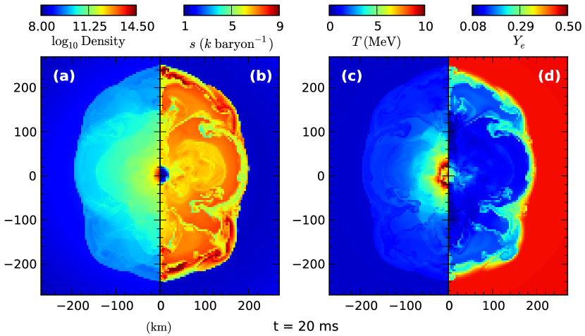
Figure 17.— Snapshot at 20 ms after bounce for the 2D cylindrical core-collapse supernova simulation. We show (a) logarithmic density, (b) entropy per baryon, (c) temperature, and (d) electron fraction, where the unit for density is $\mathrm{g}\>\mathrm{cm}^{-3}$. Only the inner 270 km of the model is shown here.

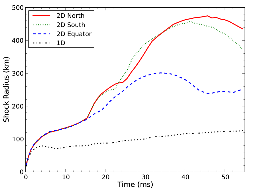
Figure 18.— Shock radius vs. post-bounce time for the 2D core-collapse supernova simulation. We show the shock position in the northern hemisphere (red solid line), southern hemisphere (green dotted line), and equatorial plane (blue dashed lines) for the 2D simulation. Also shown is the result of the 1D low-resolution simulation (black dash-dotted line).

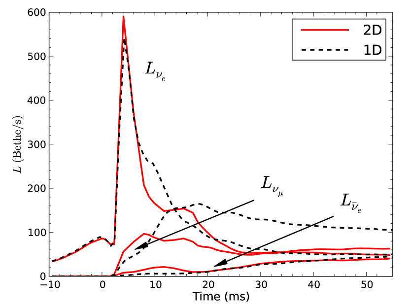
Figure 19.— Comoving frame luminosities of $\nu_{e}$, $\bar{\nu}_{e}$, and $\nu_{\mu}$ neutrinos measured at 500 km for the 2D cylindrical (red solid lines) and the low resolution 1D spherical (black dashed lines) core-collapse supernova simulations.

Since this paper is not on core-collapse supernova explosions per se, the 2D simulation is stopped at $\sim 55\>\mathrm{ms}$ after bounce. A detailed analysis of the 2D simulation is beyond the scope of this paper on algorithm, implementation, and testing.

5. Parallel Performance

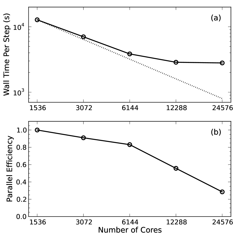
Figure 20.— Strong scaling behavior of 3D simulations on Hopper at NERSC. We show (a) wall clock time per coarse time step and (b) parallel efficiency in circles for five runs with the number of cores ranging from 1536 to 24576. The dotted line in panel (a) indicates perfect scaling.

In paper II, we demonstrated that the gray radiation solver in CASTRO has very good scaling behavior on up to 32768 cores via a weak scaling study. The multigroup radiation solver presented in this paper has similar good weak scaling behavior because the same module for solving Equation (65) is used in both solvers. Here we present a strong scaling study that was carried out on Hopper, a petascale Cray XE6 supercomputer at the National Energy Research Scientific Computing Center. We have performed a series of three-dimensional core-collapse supernova simulations in Cartesian coordinates with the same resolution on various numbers of cores. A hybrid MPI/OpenMP approach with 6 OpenMP threads per MPI task was used for these simulations. PFMG, a parallel multigrid solver from hypre (Falgout & Yang, 2002; hypre Code Project, 2012), was used to solve the linear systems. In each run, we start the 3D simulation from the result of a 1D simulation at about 10 ms before bounce. We use 12 energy groups for each species ($\nu_{e}$, $\bar{\nu}_{e}$, and $\nu_{\mu}$). The computational domain is a three-dimensional box with a size of $5000\>\mathrm{km}$ in each dimension. Three refinement levels (four total levels) are used with a refinement factor of 2 between level 0 and level 1, and a refinement factor of 4 for other levels. The coarsest level has $256^{3}$ cells. The finest level, which approximately covers the inner region of $\sqrt{x^{2}+y^{2}+z^{2}}<165\;\mathrm{km}$, has a cell size of $0.61\>\mathrm{km}$. Figure 20 shows the wall clock time per coarse time step for a series of runs with the number of cores ranging from 1536 to 24576. Also shown in Figure 20 is parallel efficient defined as

$$E(N)=\frac{N_{0}T_{0}}{NT_{N}},$$ (112)

where $N$ is the number of cores, $T_{N}$ is the wall clock time for the $N$-core run, $N_{0}$ is the number of cores in a baseline run (i.e., 1536-core run), and $T_{0}$ is the wall clock time for the baseline run. In this strong scaling study, good scaling behavior is achieved on up to $\sim 10000$ cores. However, because this is a strong scaling study, the work load per core diminishes as more cores are used. For example, the average number of cells for each core in the 24576-core run is about $16^{3}$. An unfavorable consequence of small computational boxes is an increased communication overhead. Another unfavorable consequence is that more computation is wasted at domain boundaries due to larger surface area to volume ratios of smaller boxes. Hence, the degradation of parallel performance on more than 10000 cores is not surprising.

6. Summary

In this paper, we have presented a multi-dimensional multigroup radiation hydrodynamics solver that is part of the CASTRO code. Block-structured AMR is utilized in CASTRO. In this paper, we focus attention on the single-level algorithms because the AMR algorithms have been presented in Papers I, II, and references therein.

Our multigroup radiation hydrodynamics solver is based on a comoving frame formulation that is correct to order $O(v/c)$, and uses a FLD approximation. Our mathematical analysis shows that the system we solve contains a hyperbolic subsystem that is the usual hydrodynamics system modified by radiation, a frequency space advection part that accounts for the Doppler shift of radiation due to the motion of matter, and a parabolic diffusion part. We have presented the mathematical characteristics of the hyperbolic subsystem. The eigenvalues and eigenvectors we have obtained are useful for characteristic-based Godunov schemes. We also described our treatment of the frequency space advection part. An implicit solver involving two nested iterations is presented. We have also presented two acceleration schemes that improve the convergence rate of the implicit solver.

Extensive testing is presented demonstrating the accuracy and stability of CASTRO to solve multigroup radiation hydrodynamics problems. We have presented a series of photon radiation test problems that cover a wide range of regimes. In addition to photon radiation problems, we have demonstrated the applicability of CASTRO in core-collapse supernova simulations.

Recently, Lentz et al. (2012) have argued, via a series of 1D simulations, that general relativistic effects and inelastic scattering of neutrinos on matter have significant effects on the numerical modeling of core-collapse supernova explosions. In contrast, Nordhaus et al. (2010) have concluded that spatial dimensionality has far more impact than general relativistic effects or microphysics such as inelastic scattering. Our 1D simulations are consistent with the assessment of Lentz et al. (2012) on the effects of inelastic scattering. However, our 2D simulation supports the assessment of Nordhaus et al. (2010) on the importance of spatial dimensionality. Our simulations have shown that multidimensional effects (e.g., convective motion in the region behind the shock and exterior to the nascent neutron star) appear less than 10 milliseconds after bounce, and 2D results are profoundly different from 1D results. Thus, one should be cautious about assessment of various effects such as inelastic scattering that are based on 1D simulations that last several hundred milliseconds past bounce like the ones presented in Lentz et al. (2012).

The main advantages of the CASTRO code are the efficiency due to the use of AMR and the accuracy due to the coupling of radiation force into the Riemann solver. Three-dimensional multigroup neutrino radiation hydrodynamics simulations of core-collapse supernovae with a good resolution using CASTRO can be carried out, if not now, in the near future with faster computers. In the strong scaling study with a total of 36 radiation groups and a cell size of $0.6\>\mathrm{km}$ on the finest level (Section 5), it took about 0.8 hours to advance one coarse time step (about $0.1\>\mathrm{ms}$) on 12288 cores of Hopper. Thus, it would take 800 hours on 12288 cores of Hopper to evolve to $100\>\mathrm{ms}$. Admittedly, it is still very expensive to perform long-duration 3D simulations, but it is possible to study the first $100\>\mathrm{ms}$ after bounce and investigate the development of turbulent convection region via 3D simulations.

References

- Abdikamalov et al. (2012) Abdikamalov, E., Burrows, A., Ott, C. D., Löffler, F., O’Connor, E., Dolence, J. C., & Schnetter, E. 2012, ApJ, accepted
- Alme & Wilson (1973) Alme, M. L., & Wilson, J. R. 1973, ApJ, 186, 1015
- Almgren et al. (1998) Almgren, A., Bell, J. B., Colella, P., Howell, L. H., & Welcome, M. L. 1998, Journal of Computational Physics, 142, 1
- Almgren et al. (2010) Almgren, A. S. et al. 2010, ApJ, 715, 1221
- Bell et al. (1989) Bell, J. B., Colella, P., & Trangenstein, J. A. 1989, Journal of Computational Physics, 82, 362
- Bethe (1990) Bethe, H. A. 1990, Reviews of Modern Physics, 62, 801
- Bowers & Wilson (1982) Bowers, R. L., & Wilson, J. R. 1982, ApJS, 50, 115
- Bruenn (1985) Bruenn, S. W. 1985, ApJS, 58, 771
- Bruenn et al. (1978) Bruenn, S. W., Buchler, J. R., & Yueh, W. R. 1978, Ap&SS, 59, 261
- Buchler (1983) Buchler, J. R. 1983, J. Quant. Spec. Radiat. Transf., 30, 395
- Buras et al. (2006) Buras, R., Rampp, M., Janka, H.-T., & Kifonidis, K. 2006, A&A, 447, 1049
- Burrows et al. (1995) Burrows, A., Hayes, J., & Fryxell, B. A. 1995, ApJ, 450, 830
- Burrows et al. (2007) Burrows, A., Livne, E., Dessart, L., Ott, C. D., & Murphy, J. 2007, ApJ, 655, 416
- Burrows et al. (2006) Burrows, A., Reddy, S., & Thompson, T. A. 2006, Nuclear Physics A, 777, 356
- Burrows et al. (2000) Burrows, A., Young, T., Pinto, P., Eastman, R., & Thompson, T. A. 2000, ApJ, 539, 865
- Castor (2004) Castor, J. I. 2004, Radiation Hydrodynamics (Cambridge, UK: Cambridge University Press)
- Clark (1987) Clark, B. A. 1987, Journal of Computational Physics, 70, 311
- Colella et al. (1997) Colella, P., Glaz, H. M., & Ferguson, R. E. 1997, unpublished manuscript
- Eisenstat (1981) Eisenstat, S. C. 1981, SIAM Journal on Scientific and Statistical Computing, 2, 1
- Falgout & Yang (2002) Falgout, R., & Yang, U. 2002, in Lecture Notes in Computer Science, Vol. 2331, Computational Science — ICCS 2002, ed. P. Sloot, A. Hoekstra, C. Tan, & J. Dongarra (Springer Berlin / Heidelberg), 632–641
- Fryer et al. (2006) Fryer, C. L., Rockefeller, G., & Warren, M. S. 2006, ApJ, 643, 292
- Fryer & Warren (2002) Fryer, C. L., & Warren, M. S. 2002, ApJ, 574, L65
- Gittings et al. (2008) Gittings, M. et al. 2008, Computational Science and Discovery, 1, 015005
- Graziani (2008) Graziani, F. 2008, in Lecture Notes in Computational Science and Engineering, Vol. 62, Computational Methods in Transport: Verification and Validation, ed. F. Graziani (Springer Berlin Heidelberg), 151–167
- Harten et al. (1983) Harten, A., Lax, P. D., & van Leer, B. 1983, SIAM Review, 25, 35
- Herant et al. (1994) Herant, M., Benz, W., Hix, W. R., Fryer, C. L., & Colgate, S. A. 1994, ApJ, 435, 339
- Hubeny & Burrows (2007) Hubeny, I., & Burrows, A. 2007, ApJ, 659, 1458
- hypre Code Project (2012) hypre Code Project. 2012, http://www.llnl.gov/CASC/hypre/
- Janka (2012) Janka, H.-T. 2012, Annual Review of Nuclear and Particle Science, 62, in press
- Janka et al. (2007) Janka, H.-T., Langanke, K., Marek, A., Martínez-Pinedo, G., & Müller, B. 2007, Phys. Rep., 442, 38
- Kershaw (1976) Kershaw, D. S. 1976, Flux Limiting Nature’s Own Way, Tech. Rep. UCRL-78378, Lawrence Livermore National Laboratory
- Kotake et al. (2006) Kotake, K., Sato, K., & Takahashi, K. 2006, Reports on Progress in Physics, 69, 971
- Krumholz et al. (2007) Krumholz, M. R., Klein, R. I., McKee, C. F., & Bolstad, J. 2007, APJ, 667, 626
- Lentz et al. (2012) Lentz, E. J., Mezzacappa, A., Bronson Messer, O. E., Liebendörfer, M., Hix, W. R., & Bruenn, S. W. 2012, ApJ, 747, 73
- LeVeque (2002) LeVeque, R. J. 2002, Finite-Volume Methods for Hyperbolic Problems (Cambridge University Press)
- Levermore (1984) Levermore, C. D. 1984, Journal of Quantitative Spectroscopy and Radiative Transfer, 31, 149
- Levermore & Pomraning (1981) Levermore, C. D., & Pomraning, G. C. 1981, ApJ, 248, 321
- Liebendörfer et al. (2004) Liebendörfer, M., Messer, O. E. B., Mezzacappa, A., Bruenn, S. W., Cardall, C. Y., & Thielemann, F.-K. 2004, ApJS, 150, 263
- Liebendörfer et al. (2001) Liebendörfer, M., Mezzacappa, A., Thielemann, F.-K., Messer, O. E., Hix, W. R., & Bruenn, S. W. 2001, Phys. Rev. D, 63, 103004
- Livne et al. (2004) Livne, E., Burrows, A., Walder, R., Lichtenstadt, I., & Thompson, T. A. 2004, ApJ, 609, 277
- Lowrie & Edwards (2008) Lowrie, R. B., & Edwards, J. D. 2008, Shock Waves, 18, 129
- Marek & Janka (2009) Marek, A., & Janka, H.-T. 2009, ApJ, 694, 664
- Marinak et al. (2001) Marinak, M. M., Kerbel, G. D., Gentile, N. A., Jones, O., Munro, D., Pollaine, S., Dittrich, T. R., & Haan, S. W. 2001, Physics of Plasmas, 8, 2275
- Mezzacappa & Bruenn (1993) Mezzacappa, A., & Bruenn, S. W. 1993, ApJ, 405, 669
- Mihalas & Mihalas (1999) Mihalas, D., & Mihalas, B. W. 1999, Foundations of radiation hydrodynamics (New York: Dover)
- Miller et al. (1993) Miller, D. S., Wilson, J. R., & Mayle, R. W. 1993, ApJ, 415, 278
- Miller & Colella (2002) Miller, G. H., & Colella, P. 2002, Journal of Computational Physics, 183, 26
- Minerbo (1978) Minerbo, G. N. 1978, J. Quant. Spec. Radiat. Transf., 20, 541
- Morel et al. (1985) Morel, J., Larsen, E. W., & Matzen, M. K. 1985, J. Quant. Spec. Radiat. Transf., 34, 243
- Morel et al. (2007) Morel, J. E., Brian Yang, T.-Y., & Warsa, J. S. 2007, Journal of Computational Physics, 227, 244
- Nordhaus et al. (2010) Nordhaus, J., Burrows, A., Almgren, A., & Bell, J. 2010, ApJ, 720, 694
- O’Connor & Ott (2010) O’Connor, E., & Ott, C. D. 2010, Classical and Quantum Gravity, 27, 114103
- Ott et al. (2008) Ott, C. D., Burrows, A., Dessart, L., & Livne, E. 2008, ApJ, 685, 1069
- Rampp & Janka (2000) Rampp, M., & Janka, H.-T. 2000, ApJ, 539, L33
- Rampp & Janka (2002) —. 2002, A&A, 396, 361
- Sanchez & Pomraning (1991) Sanchez, R., & Pomraning, G. C. 1991, J. Quant. Spec. Radiat. Transf., 45, 313
- Shen et al. (1998a) Shen, H., Toki, H., Oyamatsu, K., & Sumiyoshi, K. 1998a, Nuclear Physics A, 637, 435
- Shen et al. (1998b) —. 1998b, Progress of Theoretical Physics, 100, 1013
- Shestakov & Bolstad (2005) Shestakov, A. I., & Bolstad, J. H. 2005, J. Quant. Spec. Radiat. Transf., 91, 133
- Shestakov & Offner (2008) Shestakov, A. I., & Offner, S. S. R. 2008, Journal of Computational Physics, 227, 2154
- Shu & Osher (1988) Shu, C.-W., & Osher, S. 1988, Journal of Computational Physics, 77, 439
- Su & Olson (1999) Su, B., & Olson, G. L. 1999, J. Quant. Spec. Radiat. Transf., 62, 279
- Swesty & Myra (2009) Swesty, F. D., & Myra, E. S. 2009, ApJS, 181, 1
- Takiwaki et al. (2012) Takiwaki, T., Kotake, K., & Suwa, Y. 2012, ApJ, 749, 98
- Thompson et al. (2003) Thompson, T. A., Burrows, A., & Pinto, P. A. 2003, ApJ, 592, 434
- van der Holst et al. (2011) van der Holst, B. et al. 2011, ApJS, 194, 23
- van Leer (1977) van Leer, B. 1977, Journal of Computational Physics, 23, 276
- Woosley & Weaver (1995) Woosley, S. E., & Weaver, T. A. 1995, ApJS, 101, 181
- Zhang et al. (2011) Zhang, W., Howell, L., Almgren, A., Burrows, A., & Bell, J. 2011, ApJS, 196, 20