The Envelope and Embedded Disk around the Class 0 Protostar L1157-mm: Dual-wavelength Interferometric Observations and Modeling

Abstract

We present dual-wavelength observations and modeling of the nearly edge-on Class 0 young stellar object L1157-mm. Using the Combined Array for Research in Millimeter-wave Astronomy, a nearly spherical structure is seen from the circumstellar envelope at the size scale of 10² to 10³ AU in both 1 mm and 3 mm dust emission. Radiative transfer modeling is performed to compare data with theoretical envelope models, including a power-law envelope model and the Terebey-Shu-Cassen model. Bayesian inference is applied for parameter estimation and information criteria is used for model selection. The results prefer the power-law envelope model against the Terebey-Shu-Cassen model. In particular, for the power-law envelope model, a steep density profile with an index of $\sim$2 is inferred. Moreover, the dust opacity spectral index $\beta$ is estimated to be $\sim$0.9, implying that grain growth has started at L1157-mm. Also, the unresolved disk component is constrained to be $\lesssim$ 40 AU in radius and $\lesssim$ 4-25 M_Jup in mass. However, the estimate of the embedded disk component relies on the assumed envelope model.

1 Introduction

Protostars are surrounded by their natal envelopes in the earliest stage of evolution. These envelopes supply the material that is actively infalling onto the embedded star-disk system, and their properties can affect the subsequent evolution. Much theoretical work has been done to address the collapse process and the physical properties of the envelope, varying from self-similar solutions to numerical calculations including rotation and magnetic fields (e.g., Larson, 1969; Penston, 1969; Hunter, 1977; Shu, 1977; Terebey et al., 1984; Whitworth & Summers, 1985; Galli & Shu, 1993; Masunaga & Inutsuka, 2000; Tassis & Mouschovias, 2005; Hennebelle & Fromang, 2008). While various theoretical models of the collapsing envelope have been suggested, distinguishing between the suggested theoretical models has always been an observational challenge. For example, the model of Terebey, Shu, & Cassen (1984, hereafter the TSC model) has been widely used and consistent results have been obtained, especially in fitting the spectral energy distributions of unresolved young stellar objects (e.g., Robitaille et al., 2007), but it is based on the Shu (1977) model, which could not fit a sample of Class 0 protostars with reasonable ages. (Looney et al. 2003).

To better constrain the envelope structure, we carry out complete modeling with dual-wavelength millimeter data. At such wavelengths, the continuum is dominated by dust emission from the envelope and the embedded disk. Interferometry is a useful tool to probe the structure of protostellar envelopes as it measures emission at various spatial scales, leading to a more complete analysis for the envelope. By comparing the predicted envelope structure with interferometric observations, theoretical collapse models can be tested (e.g., Chiang et al., 2008; Maury et al., 2010). A better understanding of the envelope also enables us to constrain the physical properties of the embedded disk component.

In this paper, we focus on the edge-on Class 0 protostar L1157-mm (also known as L1157-IRS or IRAS 20386+6751). The distance to L1157-mm is around 200-450 pc (Straizys et al., 1992; Kun, 1998; Kun et al., 2008); here we follow Looney et al. (2007) and adopt 250 pc. A chemically active outflow driven by L1157-mm has been detected in multiple species (Gueth et al., 1996; Bachiller et al., 2001; Nisini et al., 2010). Perpendicular to the outflow orientation, a flattened envelope with a linear size of $\sim$20,000 AU is seen in 8 $\mu$m absorption, N₂H⁺ emission, and NH₃ emission, showing complex kinematics from rotation, infall, and outflow in the envelope (Looney et al., 2007; Chiang et al., 2010; Tobin et al., 2011). On the other hand, dust continuum traces the envelope structure as well as reveals a compact core (e.g., Gueth et al., 2003). Additionally, the presence of a circumstellar disk embedded inside the envelope is suggested by methanol observations (Goldsmith et al., 1999; Velusamy et al., 2002).

We have collected 1 mm and 3 mm interferometric data at multiple array configurations using the Combined Array for Research in Millimeter-wave Astronomy (CARMA; Woody et al., 2004) . §2 gives an overview of the observations and the data reduction. Details of the modeling are addressed in §3 with a further supplement on our statistical approach in the Appendix. The results are presented in §4, their implications are discussed in §5, and a summary is given in §6.

2 Observations and Data Reduction

L1157-mm was observed by the 15-element CARMA between Oct 2007 and Jan 2010. At that time, the science array of CARMA consisted of six 10.4-meter antennas and nine 6.1-meter antennas. Dust continuum at both 1 mm and 3 mm bands was observed using multiple array configurations, as summarized in Table 1.

Table 1: Summary of Observations

Frequency	Array	Date	Observing	Bandpass	Flux	Beam Size	Beam P.A.
(GHz)	Config.		Time (hr)	Calibrator	Calibrator	($\arcsec$)	(degree)
(1)	(2)	(3)	(4)	(5)	(6)	(7)	(8)
229	B	2007-12-17	1.5	3C454.3	MWC349	0.4$\times$0.3	-75
	C	2008-04-13	3.1	3C454.3	MWC349	1.0$\times$0.8	-66
	D	2008-03-07	3.1	3C454.3	MWC349	2.3$\times$2.0	-29
91	A	2009-01-27	3.3	1642+689	MWC349	0.4$\times$0.3	-65
		2010-01-26	2.2	3C273	MWC349
		2010-02-01	2.9	3C454.3	Neptune
	B	2007-11-17	4.5	1751+096	MWC349	0.9$\times$0.8	-83
		2007-11-19	2.4	3C454.3	Neptune
		2007-11-20	1.5	3C273	3C273
		2009-12-14	0.6	3C454.3	Uranus
		2009-12-15	5.4	3C345	MWC349
	C	2007-10-03	2.5	1751+096	MWC349	2.3$\times$2.0	-87
		2007-10-05	2.8	1751+096	MWC349
		2008-04-05	4.8	3C273	MWC349
	D	2008-02-29	3.1	3C454.3	Uranus	6.0$\times$5.2	84
		2009-03-19	6.0	3C345	MWC349
		2009-03-20	6.2	3C345	MWC349
		2009-03-27	0.8	1642+689	MWC349
		2009-03-29	3.0	1642+689	MWC349
	E	2008-10-02	4.2	3C454.3	Uranus	11.5$\times$10.2	78
		2008-10-05	3.5	3C84	MWC349

The phase center of the observations before September 2008 was $\alpha$ = 20^h39^m06$\fs$20, $\delta$ = 68°02′15$\farcs$9, and shifted to $\alpha$ = 20^h39^m06$\fs$26, $\delta$ = 68°02′15$\farcs$8 afterwards as more precise coordinates were determined by high resolution observations. However, all data presented here have been corrected to have the common phase center at $\alpha$ = 20^h39^m06$\fs$26, $\delta$ = 68°02′15$\farcs$8 (J2000).

The main phase calibrator for all tracks was 1927+739 (with the exception of one A-array track) and was observed with a phase calibrator-source cycle of 10-15 minutes. For all A- and B-array observations, a weaker quasar, 2009+724, was observed as the secondary phase calibrator. The secondary phase calibrator was not used in the calibration process; instead, it is used to check the point source response. For 3 mm A- and B-array tracks observed in winter 2009-2010, the CARMA Paired Antenna Calibration System (C-PACS; Pérez et al., 2010) was employed to calibrate the atmospheric phase variation on short time-scale. With C-PACS, a reference array continuously monitors a nearby quasar, called the atmospheric calibrator, for atmospheric delay, while the science array observes the science target. The eight 3.5-meter antennas, from the previous Sunyaev-Zel’dovich Array (SZA), were used as the reference array. The C-PACS correction is effective for data with long baseline.

The data reduction, calibration, and imaging were done using the Multichannel Image Reconstruction, Image Analysis and Display package (MIRIAD; Sault et al., 1995). The bandpass and flux calibrators for each track are listed in Table 1. After the data are reduced, the flux density of both primary and secondary phase calibrators is plotted as a function of $u$-$v$ distance in order to verify a flat trend, implying that decorrelation is not significant at long baselines.

The largest uncertainty of interferometric data comes from flux or absolute amplitude calibration. Although independent of relative brightness and image quality for one track of data, it affects the analysis through the differences between tracks. The uncertainty can be larger than 10% mostly due to the planetary model of the flux calibrator used in the data reduction process (e.g., Moreno & Guilloteau, 2002). The large uncertainty cannot be avoided unless the planet modeling is improved. The flux uncertainty can affect the analysis through (1) the uncertainty between tracks at the same wavelength, and (2) the uncertainty between tracks at different wavelengths. The uncertainty of the first kind can affect the deduced envelope and disk structure in the modeling. To ensure its impact is minimized, we compare the flux of the common phase calibrator 1927+739 among tracks. At each wavelength, we verify that the flux value varies smoothly in time and is consistent with the flux reported in the standard CARMA/MIRIAD catalog. Also, data and model are compared at each visibility point, so the uncertainties are better preserved compared to modeling using binned visibilities (see §3.5). For the rest of the paper we consider the absolute flux uncertainty of the second kind for dual-wavelength analysis. A 10% uncertainty for the absolute flux at each wavelength is adopted. It dominates errors in estimating spectral parameter, such as the dust opacity spectal index, as will be seen in §4. Other model parameters can be affected directly or indirectly through the uncertainty of the spectral parameter. Other systematic uncertainty from instruments and calibrations may exist and propagate in the analysis as well, but are presumably less than 10%.

The reduced data of the science target L1157-mm are shown in Figure 1 by the annuli-averaged flux density with respect to $u$-$v$ distance. Continuum data from all spectral windows are combined. Figure 2 presents the continuum maps of L1157-mm. Super-uniform weightings with different robustness parameters are used to obtain different synthesized beamsizes in order to emphasize envelope structures at different size scales. The continuum of L1157-mm shows spherical structures from 2000 AU scale (8″) down to 100 AU scale (0.4″). In panel (f), the envelope structure is slightly elongated perpendicular to the outflow direction, but the larger-scale extended envelope, detected by IRAM 30-m telescope (Gueth et al., 2003) and SMA (with lower resolution than our CARMA observations; Tobin et al. in preparation), is not seen in our CARMA dust continuum data. No apparent disk or flattened structure is seen at small scale either.

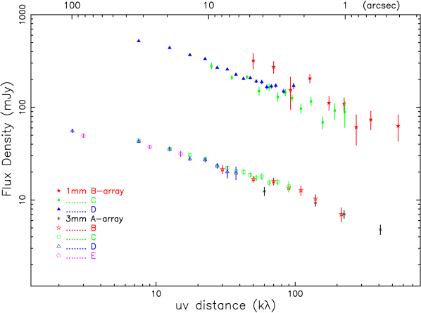
Figure 1: Flux density of L1157-mm dust continuum at 1 mm (filled symbols) and 3 mm (open symbols). The visibilities are vector averaged around the source center and binned into u-v annuli. Data collected in different array configurations are plotted separately. The error bars show only the statistical errors within each annuli-bin, while the typical uncertainty carried by single data visibility is around 0.2-2.5 Jy.

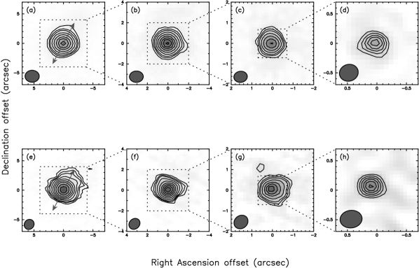
Figure 2: CARMA 3 mm (upper) and 1 mm (lower) dust continuum images of L1157-mm. The same multi-configuration data with different u-v imaging weightings are shown to emphasize structures on different size scales. The contour levels, noise rms ($\sigma$), and beams are as follows: (a) [3,4,5,7,10,14,18,22]$\times\sigma$, $\sigma=$ 0.9 mJy beam^-1, 2.40$\arcsec\times$2.03$\arcsec$ at a position angle of 90^∘; (b) [3,4,5,7,10,14,18,22,26]$\times\sigma$, $\sigma=$ 0.6 mJy beam^-1, 1.34$\arcsec\times$1.10$\arcsec$ at a position angle of -88^∘; (c) [3,4,5,7,10,14,18]$\times\sigma$, $\sigma=$ 0.6 mJy beam^-1, 0.65$\arcsec\times$0.54$\arcsec$ at a position angle of -82^∘; (d) [3,4,5,6,7]$\times\sigma$, $\sigma=$ 0.9 mJy beam^-1, 0.32$\arcsec\times$0.28$\arcsec$ at a position angle of -73^∘. (e) [3,4,5,7,10,14,20,30,42]$\times\sigma$, $\sigma=$4.0 mJy beam^-1, 1.77$\arcsec\times$1.61$\arcsec$ at a position angle of -38^∘; (f) [3,4,5,7,10,14,18,22,26]$\times\sigma$, $\sigma=$5.5 mJy beam^-1, 1.14$\arcsec\times$0.98$\arcsec$ at a position angle of -48^∘; (g) [3,4,5,7,10,13,16]$\times\sigma$, $\sigma=$ 7.0 mJy beam^-1, 0.71$\arcsec\times$0.62$\arcsec$ at a position angle of -51^∘; (h) [3,4,5,6,7,8]$\times\sigma$, $\sigma=$ 12.0 mJy beam^-1, 0.37$\arcsec\times$0.30$\arcsec$ at a position angle of -83^∘.

3 Aspects of Modeling a Class 0 YSO

To compare a YSO model with observations, we consider the physical conditions of the system, including the density and temperature structures (§3.1 and §3.2) and dust grain properties (§3.3). The radiative transfer tool RADMC-3D, developed by C. P. Dullemond and co-authors (Dullemond & Dominik, 2004) , is used. Observational effects from the interferometer are taken into account and a Bayesian approach is taken for model fitting (§3.5). In the following sections, we discuss the details of each facet in the modeling.

3.1 Envelope Structure

A simple Class 0 YSO model consisting of a spherical dusty envelope, a bipolar outflow, and possibly a circumstellar disk is considered. For the envelope structures, we examine a simple power-law density profile, representing self-similar collapse solutions, and a collapse with rotation (Terebey et al. 1984). An unresolved component is included to represent a compact disk structure.

To include a simple bipolar outflow cavity in the model, we remove material orientated with the observed envelope geometry and outflow properties: a position angle of 152° for the outflow-axis cut, an inclination angle of 80°, and an opening angle 30° for the outflow cavity are assumed (Choi et al., 1999; Gueth et al., 1996, 1997). For simplicity, the inner and outer radii of the envelope are fixed to be 12 AU and 10,000 AU, respectively. The inner envelope cavity is smaller than the highest observational resolution, and always within the central cell in the model images. A large outer radius is adopted so there is no ringing effect due to interferometric response on a sharp cutoff in the envelope. Additionally, as the density and temperature are much lower in the outer envelope, precise choice of the outer radius does not play an important role at these wavelengths.

3.2 Temperature Structure

While many theoretical models ignore the internal heating from the newborn protostar, it is critical to take into account the protostellar contribution to agree with observational luminosity (Adams & Shu, 1985). The heating and cooling of dust grains, dominated by the central illumination and dust grain properties, should be balanced to obtain an equilibrium temperature. To simulate millimeter-wave observations of protostars surrounded by dusty environments, such a realistic temperature distribution needs to be either assumed or calculated.

The temperature structure can be approximated assuming simple conditions of the dusty envelope. Assuming a centrally illuminated spherical envelope in which the density has a power-law dependence on radius,

$$\rho(r)=\rho_{0}\left(\frac{r}{r_{0}}\right)^{-p},$$ (1)

where $\rho_{0}$ is the density at an arbitrary radius $r_{0}$ and $p$ is the density power-law index, and assuming a pure power-law dust opacity with a spectral index $\beta$, the temperature structure in the optically thin outer envelope can be approximated by

$$T(r)=T_{0}\left(\frac{r}{r_{0}}\right)^{-\frac{2}{\beta+4}}$$ (2)

(Wolfire & Cassinelli, 1986; Adams, 1991).

However, if the assumptions of power-law dust opacity and spherical power-law density do not hold, the approximation in Eq. (2) can be inadequate even in the optically thin reion. For example, the dust opacity is not a pure power-law at short wavelengths, and the density structure can also be more complicated than the power-law profile. Furthermore, Eq. (2) is only valid in the optically thin region and relies on $T_{0}$ at $r_{0}$. With a fixed central heating source, $T_{0}$ at $r_{0}$ is characterized by the optically thick-thin transition zone, and is difficult to estimate without a good understanding of the optically thick inner region.

Given the difficulty to approximate the temperature structure with a variety of envelope models and ranges of model parameters, we calculate a self-consistent temperature distribution for each set of parameters using the Monte Carlo radiative transfer code RADMC-3D (Dullemond & Dominik, 2004). A luminosity of 8.4 L_⊙ is adopted (Froebrich, 2005) as a fixed input in the radiative transfer calculation. This bolometric luminosity can be underestimated due to insufficient sampling of the spectral energy distribution, but can be overestimated due to a larger assumed distance. Furthermore, the intrinsic luminosity can be larger than the measured bolometric luminosity due to the source’s edge-on orientation (e.g., see more discussions in Froebrich, 2005; Whitney et al., 2003). Despite the uncertainty in luminosity, a self-consistent temperature structure is the best compromise for now.

3.3 Dust Grain Properties

Dust grain properties such as chemical composition, geometry, alignment, degree of ionization, and size distribution play important roles in star-forming processes from thermodynamics and grain surface chemistry to timescales of magnetic field effects. For dust grains in the diffuse interstellar medium, the classic model constructed by Mathis, Rumpl, & Nordsieck (1977, hereafter MRN) with optical constants calculated by Draine & Lee (1984) can reproduce the interstellar extinction and polarization observations from infrared to ultraviolet wavelengths. However, for dust grains in dense cores and star forming regions, collisions and interactions between grain particles become more important. Ossenkopf & Henning (1994) has considered the dust coagulation process in dense protostellar cores and found that the opacity can be enhanced by a factor of a few as grains aggregate. The authors started with the MRN grains covered with different amounts of ice mantles, and investigated the optical constants after $10^{5}$ yrs of coagulation in gas densities ranging from $10^{5}$ to $10^{8}$ cm^-3.

In our modeling, we adopt the dust opacity, or the mass absorption coefficient $\kappa$ defined as the cross section per unit mass, from column 5 of Table 1 in Ossenkopf & Henning (1994), the so-called OH5 grain which is covered by a thin layer of ice mantle and coagulated at $10^{6}$ cm^-3. Besides being widely used, the OH5 model shows agreements with, and in some cases favored by, multi-wavelength observations of star-forming regions (e.g., van der Tak et al., 1999; Evans et al., 2001; Shirley et al., 2005, 2011a).

At far-infrared and millimeter wavelengths, $\kappa$ can be approximated as a power law with respect to frequency

$$\kappa=\kappa_{0}\left(\frac{\nu}{\nu_{0}}\right)^{\beta}.$$ (3)

This sub-millimeter dust opacity spectral index $\beta$, which can only be studied with multi-wavelength observations, varies with environment and is related to grain properties mentioned previously. $\beta$ is $\gtrsim$ 1.7 in the diffuse interstellar medium and starless cores (e.g., Draine & Lee, 1984; Schnee et al., 2010), but significantly lower in protoplanetary disks ($\beta~{}\lesssim~{}$1, e.g., Beckwith & Sargent, 1991; Natta et al., 2007; Ricci et al., 2010b). One explanation for lower $\beta$ is a larger grain size and more discussions will be in §5.4. In order to better understand the dust property of L1157-mm, we include $\beta$ as a model parameter. Based on the OH5 model, we modify the opacity curve with a power-law of index $\beta$ as in Eq. (3) at wavelengths longer than an arbitrary choice of 700 $\mu$m.

The dust opacity used in the analysis can substantially affect the deduced spectral energy distribution as well as temperature structure of YSOs. With the radiative transfer tool, we find that the temperature structure is mostly determined by the dust opacity at short wavelengths. $\beta$, which characterizes the dust property at long wavelengths, plays a less important role for the temperature structure; instead, $\beta$ affects the observed flux directly through dust opacity (Chandler et al., 1998).

With the optically thin assumption, $\beta$ can be estimated using flux ratio between two wavelengths in the Rayleigh-Jeans regime; here we call the approximate dust opacity spectral index $\beta_{thin}$. In this limit, the flux density $F_{\nu}\propto\kappa_{\nu}B_{\nu}\propto\nu^{\beta_{thin}+2}$; therefore,

$$\beta_{thin}=\frac{\ln F_{1}-\ln F_{2}}{\ln\nu_{1}-\ln\nu_{2}}-2$$ (4)

(e.g., Kwon et al., 2009). Figure 3 shows $\beta_{thin}$ of L1157-mm using the annuli-averaged visibility at each u-v distance bin of our dual-wavelength data. The uncertainty of the $\beta_{thin}$ estimation is discussed in Appendix A. $\beta_{thin}$ is a good approximation in the optically thin region, but a correction term is needed in the optically thick region (e.g., Rodmann et al., 2006; Lommen et al., 2007). To avoid the need of the correction term, full optical depth effect is considered in our radiative transfer modeling. Nonetheless, $\beta_{thin}$ provides a quick and rough estimate for the $\beta$ value across the envelope and reveals possible radial dependence. As seen in Figure 3, no strong radial dependence is suggested for $\beta$ at L1157-mm. Therefore, we assume uniform grain properties in the envelope model for simplicity. In other words, $\kappa$ is only a function of frequency and independent of radius in our envelope model.

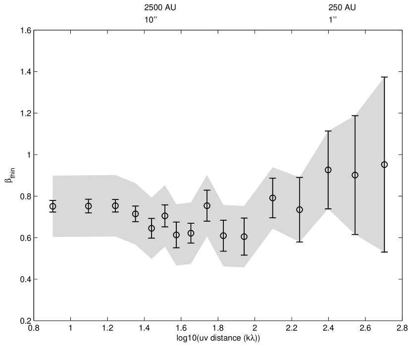
Figure 3: Approximate dust opacity spectral index $\beta_{thin}$ of L1157-mm as a function of u-v distance assuming the optically thin condition. The error bars show only the statistical errors without the absolute flux uncertainty, while the shade shows the errors including the absolute flux uncertainty.

3.4 Free-free Contamination

We ignore the contribution of free-free emission in this study. Free-free emission from ionized winds or jets can contribute partial flux at millimeter wavelengths ($\sim$20% at 7 mm, Rodmann et al., 2006) and affect model parameter estimates especially for $\beta$ and disk component. However, it plays a minimal role for our data of L1157-mm at 1 mm and 3 mm. By extrapolating fluxes at 8.5 GHz and 4.86 GHz (Meehan et al., 1998) to our observed frequency, we estimated the free-free emission to be around 0.53 mJy at 3 mm and 0.39 mJy at 1 mm for L1157-mm. The free-free correction is negligible in the analysis.

3.5 Model Fitting

Given a set of model parameters, we estimate the sky brightness distribution for the dust continuum with radiative transfer calculations. The density and self-consistent temperature distributions in three dimensions are considered along with the model dust property. Essentially, for each pixel on the plane of sky, the flux is calculated by integrating the dust emission along the line of sight (e.g., Adams, 1991). Assuming no background brightness, the specific intensity can be expressed as

$$I_{\nu}=\int_{los}B_{\nu}(T)\,e^{-\tau_{\nu}}\,\textrm{d}\tau_{\nu}=\int_{los}B_{\nu}(T(\vec{r}))\,e^{-\tau_{\nu}(\vec{r})}\,\rho(\vec{r})\,\kappa_{\nu}\,\textrm{d}\vec{r},$$ (5)

where $B_{\nu}(T)$ is the Planck function at dust temperature $T$, $\rho$ is the envelope density, $\vec{r}$ denotes the position, and $\tau_{\nu}$ is the optical depth from the position $\vec{r}$ along the line of sight ($los$) to the observer

$$\tau_{\nu}(\vec{r})=\kappa_{\nu}\int_{los}\rho(\vec{r})d\vec{r}=\kappa_{\nu}\int_{l}^{\infty}\rho(\vec{r})dl^{\prime}.$$ (6)

$T$, $\rho$, and $\tau_{\nu}$ are all dependent of $\vec{r}$.

With the model sky brightness, we simulate interferometric observations and generate model visibilities. The sky image is convolved with the primary beam patterns of the antennas and then Fourier transformed into visibilities with the observational u-v sampling. In the case of the 15-element CARMA, the 6.1-meter dishes and 10.4-meter dishes give 3 types of baselines. Therefore we construct separate primary-beam-corrected images for each kind of baseline, and sample the images with corresponding u-v spacing for each data visibility from real observations. In addition, images at two wavelengths are constructed individually based on the same model.

Model visibilities are compared with observational data at each u-v sample and wavelength. The analysis is done in the visibility domain so as to avoid the complexity brought by the CLEAN algorithm, u-v sampling, and imaging process. Some information is lost in the image domain through the imaging process, since structures in images can be sensitive to beamsize or weighting. In other words, emission at different size scales can either be emphasized or suppressed, causing biases in the model-data comparison; therefore, we perform the analysis in the visibility domain. Furthermore, visibilities are compared data point by data point; no binning nor averaging are done (e.g., Isella et al., 2009).

Assuming the noise from observations is normally distributed or Gaussian noise, the goodness of a model-fit can be characterized by the standard chi-square statistics. Real and imaginary parts of each visibility point are considered individually, as in

$$\chi^{2}=\displaystyle{\sum_{i}}\frac{(Re(V_{model,i})-Re(V_{data,i}))^{2}+(Im(V_{model,i})-Im(V_{data,i}))^{2}}{\sigma_{i}^{2}}$$ (7)

where $i$ stands for each visibility point at its unique $u$-$v$. The noise of each visibility $\sigma$ is the square root of data variance (outputted by MIRIAD task uvinfo) multiplied by a scaling factor to account for imperfect weather conditions. The noise level before the scaling follows

$$\sigma_{o}=\frac{2k_{b}T_{sys}}{\eta_{a}\eta_{c}A\sqrt{N(N-1)\Delta\nu t_{int}}},$$ (8)

where $k_{b}$ is the Boltzmann constant, $T_{sys}$ is the system temperature, $\eta_{a}$ is the aperture efficiency, $\eta_{c}$ is the correlator efficiency, $A$ is the antenna collecting area, $N$ is the number of antennas, $\Delta\nu$ is the bandwidth, and $t_{int}$ is the on-source integration time.

The scaling factor is used to correct $\sigma$ for the phase decorrelation and is 1 if no scaling is done. There are multiple ways to scale the noise, and the scaling factor should be somewhat dependent on the baseline length. In this work we determine the scaling factor by the phase scatter in each array configuration at each wavelength. Nonetheless, the factor is always larger than 1; in other words, we only adjust $\sigma$ to make data less constraining.

We take the Bayesian approach to compare data and model (e.g., Ford, 2005; Spergel et al., 2007). Given a specific model, a global minimum of $\chi^{2}$ is searched and verified to be a good fit with a chi-square hypothesis test. Then, the Markov chain Monte Carlo (MCMC) method is utilized to calculate the posterior probability distributions; in particular, the posterior-weighted value and the uncertainty are estimated for each model parameter. Details of our fitting technique are discussed in Appendix B. Note that the deduced parameters are valid only within the framework of model assumptions. Evaluating the goodness of a model and comparisons between models will be discussed in §5.1.

4 Results

In this section, the modeling results based on the details described in §3 are presented. Three models are considered and shown individually.

4.1 Spherical Power-law Envelope Model

We first consider a spherical envelope with a power-law density profile and self-consistent temperature structure. In this simplest model, three model parameters are included: (a) the dust opacity spectral index $\beta$ as in Eq. (3), (b) the dust density $\rho_{0}$ at 100 AU, which scales with the total envelope mass, and (c) the density power-law index $p$ as in Eq. (1). All other model properties are fixed as described in §3.

We begin with only considering the statistical noise of data visibility and ignoring the uncertainty of absolute flux. This is to characterize the case without absolute flux uncertainty, as well as demonstrate the effect of absolute flux uncertainty. Using the MCMC results, the expectation values and uncertainties of all parameters are estimated (Table 2), and the marginalized posterior probability distributions in 1-D and 2-D parameter space are shown in Figure 4. We choose to list the radius of the 68% confidence interval in Table 2 as it represents 1 $\sigma$. The 68% and 95% confidence regions are shown by 2-D contours to reveal any correlation between parameters. For example, as shown by the marginalized contours in the $\beta$-$\rho_{0}$ plane in Figure 4 (middle row, left column), a correlation between the dust opacity spectral index $\beta$ and the density scaling $\rho_{0}$ is implied. This is because a larger $\beta$ means a smaller dust opacity $\kappa$ in the model, resulting in larger deduced mass and thus larger density scaling.

Table 2: Power-law Envelope Model

Parameter	Mean	Radius of the 68% confidence interval
		(statistical noise only)	(with flux uncertainty)
(1)	(2)	(3)	(4)
dust opacity spectral index $\beta$	0.84037	0.00014	0.11
density at 100 AU (in 10-18 g cm-3)	8.5881	0.0013	1.2
density power-law index $p$	2.00939	0.00020	0.03

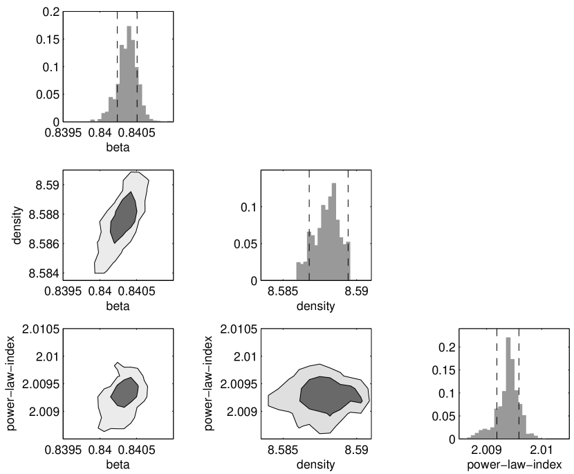
Figure 4: Marginalized posterior probability distributions for the parameters of the power-law envelope model (dust opacity spectral index $\beta$, density $\rho_{0}$ at 100 AU in the unit of 10^-18 g cm^-3, and envelope density power-law index $p$). Only the statistical errors, but not the absolute flux uncertainty, are considered for the data. In the histograms, the dashed vertical lines enclose 68% or 1 $\sigma$ confidence interval, with the expectation values and $\sigma$ listed in Table 2. The dark and light areas in the 2-D contour plots are the 68% and 95% confidence regions.

The parameters are determined with a high precision within the framework of model assumptions. The narrow uncertainties can be understood since approximately five million independent data visibilities are used to fit only three model parameters. Strong assumptions are imposed in the model. Similar results have been obtained in other studies as well. For example, Kwon et al. (2011) have taken the Bayesian approach to estimate model parameters and their errors in the applications of T-Tauri disks, and small uncertainties are obtained when only the statistical errors in the data are considered.

However, the absolute amplitude uncertainty, originated by the absolute flux calibration in the data reduction process, brings more uncertainties to the model parameter estimation. As we have verified that the calibrator flux is consistent among all observational tracks at multiple array configurations (§2), the absolute flux errors effectively cause an uncertain scaling to the amplitude of all data at each wavelength. The absolute flux uncertainty can play a dominating role in estimating frequency-dependent parameters, but cause minimal effects at the relative spatial structures probed at one single wavelength.

Marginalization in the framework of Bayesian statistics allows us to quantitatively take the absolute flux uncertainty into consideration. We introduce two additional nuisance parameters, $S_{1mm}$ and $S_{3mm}$, to scale the absolute amplitude of all data at 1 mm and 3 mm, respectively. $S_{1mm}$ = 1 and $S_{3mm}$ = 1 means no scaling is done, as in the presented dataset. Since the main uncertainty of flux calibration results from the choice of planetary models and no model is preferred, a flat probability distribution for both $S_{1mm}$ and $S_{3mm}$, ranging from 0.9 to 1.1, is assumed. The range of the scaling factors is chosen to be consistent with the commonly quoted 10% errors for the absolute flux calibration. Our approach is similar to the method of Lay et al. (1995).

Figure 5 shows the marginalized posterior probability distributions of model parameters with consideration of the absolute flux uncertainty. The uncertainties of parameters are listed in Table 2 column 4. Inclusion of absolute flux uncertainty increases the parameter errors by a factor of 2-3 orders of magnitude, and it is critical for parameter estimation as it makes data much less constraining. In particular, the dust spectral index $\beta$ is mostly determined by the flux ratio between 1 mm and 3 mm, hence it becomes much more uncertain due to the uncertainty of absolute amplitude.

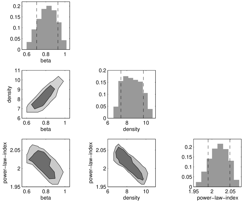
Figure 5: Same as Figure 4 but with the consideration of the absolute flux uncertainty. $\sigma$ for the model parameters are listed in Table 2 column 4.

For additional visualization, Figure 6 shows the observational data visibility of L1157-mm and the model calculated with the marginalized parameters as an a posteriori comparison. Because there are about five million data visibilities and each visibility contains low signal-to-noise, plotting them all does not show information. Therefore, visibilities are averaged vectorially and binned in $u$-$v$ annuli around the source center using the MIRIAD task uvamp. The error bars in Figure 6 are statistical errors in the bins. Note that visibility data are not averaged in the modeling process, and the binned visibility is just one data representation. The same dataset can have multiple representations depending on how they are binned, and the statistical errors in the bins may not reflect the whole uncertainty.

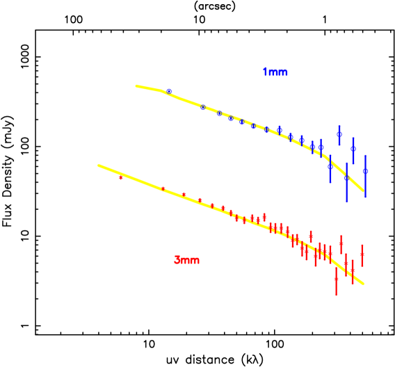
Figure 6: Flux density of the observational data (circles for 1 mm data and asterisks for 3 mm data) and the model fit (solid lines) with the marginalized parameters for the power-law envelope model. While modeling is done with non-averaged visibilities, annuli-averaged visibilities are shown as a function of $u$-$v$ distance. Error bars are statistical errors in the annuli-bins only and different from the visibility uncertainty used in the modeling.

Figure 7 and Figure 8

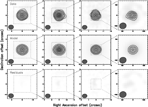
Figure 7: Comparison between 3 mm dust continuum data (upper row, as shown in Figure 2), model (middle row), and residuals (lower row) of L1157-mm in the image space. The power-law envelope model is used. Images in each column share the same u-v imaging weighting and contour levels. The contour levels, noise rms ($\sigma$), and beams are: column 1: [-3,3,4,5,7,10,14,18,22]$\times\sigma$, $\sigma=$ 0.9 mJy beam^-1, 2.40$\arcsec\times$2.03$\arcsec$ at a position angle of 90^∘; column 2: [-3,3,4,5,7,10,14,18,22,26]$\times\sigma$, $\sigma=$ 0.6 mJy beam^-1, 1.34$\arcsec\times$1.10$\arcsec$ at a position angle of -88^∘; column 3: [-3,3,4,5,7,10,14,18]$\times\sigma$, $\sigma=$ 0.6 mJy beam^-1, 0.65$\arcsec\times$0.54$\arcsec$ at a position angle of -82^∘; column 4: [-3,3,4,5,6,7]$\times\sigma$, $\sigma=$ 0.9 mJy beam^-1, 0.32$\arcsec\times$0.28$\arcsec$ at a position angle of -73^∘.

Figure 8: Comparison between 1 mm dust continuum data (upper row, as shown in Figure 2), model (middle row), and residuals (lower row) of L1157-mm in the image space. Images in each column share the same u-v imaging weighting and contour levels. The contour levels, noise rms ($\sigma$), and beams are: column 1: [-3,3,4,5,7,10,14,20,30,42]$\times\sigma$, $\sigma=$4.0 mJy beam^-1, 1.77$\arcsec\times$1.61$\arcsec$ at a position angle of -38^∘; column 2: [-3,3,4,5,7,10,14,18,22,26]$\times\sigma$, $\sigma=$5.5 mJy beam^-1, 1.14$\arcsec\times$0.98$\arcsec$ at a position angle of -48^∘; column 3: [-3,3,4,5,7,10,13,16]$\times\sigma$, $\sigma=$ 7.0 mJy beam^-1, 0.71$\arcsec\times$0.62$\arcsec$ at a position angle of -51^∘; column 4: [-3,3,4,5,6,7,8]$\times\sigma$, $\sigma=$ 12.0 mJy beam^-1, 0.37$\arcsec\times$0.30$\arcsec$ at a position angle of -83^∘. The 3 $\sigma$ residuals at the smallest-scale image (lower-right) is likely due to the differences of the emission peak position measured using 1 mm and 3 mm data, while the modeling is done around the peak position measured using 3 mm data. If we shift the model with this offset at 1 mm, no residuals is left at 3 $\sigma$ level in the small-scale image.

continue the a posteriori check and compare the model with the data in the image domain for the 3 mm and 1 mm dust continuum, respectively. We image the model visibilities in the same way the data visibilities are imaged as shown in Figure 2, that is, the same sets of u-v imaging weightings are used for showing structures at four size scales at each wavelength. Residuals in the visibility domain are also imaged and shown in Figure 7 and Figure 8 to demonstrate the fitting error in the image space. The subtraction of model from data leaves no residuals greater than 3 $\sigma$ level at the 3 mm images, confirming that a good fit is obtained. In the large-scale image of 1 mm continuum, the residuals extend towards the north-west of the protostar, which aligns with the outflow direction and is likely due to the asymmetric structure from the outflow. In the small-scale image of 1 mm continuum, a 3 $\sigma$ peak is seen to the north-east of the protostar, which is likely caused by the differences of the emission peak position measured using 1 mm and 3 mm data. We estimate the protostar position by fitting a Gaussian to the highest resolution observations at 3 mm, and there is a slight offset relative to the protostar position measured using 1 mm data. If we shift the model with this offset at 1 mm, no residuals higher than 3 $\sigma$ are left in the small-scale image.

The posterior-weighted results suggest a density power-law index $p\sim$ 2. In this case, the envelope density structure is similar to a singular isothermal sphere or the beginning stage of the Shu model with a very small infall region. In the Shu model, a free-fall-like $p\sim$ 1.5 profile is established quickly during the collapse process. If the Shu model is applied strictly, an extremely young age of $\sim$10³ yrs is implied. This age is much younger than other age estimates. For example, a kinematic age of $\sim$15,000 yrs is suggested by the outflow observations (Bachiller et al., 2001). The results are consistent with the single-wavelength study of Looney et al. (2003), in which a larger sample of Class 0 YSOs are modeled and unphysical young ages are derived using the simple self-similar model. A steep density profile can be related to a finite mass reservoir, as the constraint from an outer boundary can steepen the density in the outer envelope (Vorobyov & Basu, 2005). Another possibility is the change of dust grain properties across the envelope. If larger grains are present towards the inner envelope, their greater opacity can result in a steeper density profile being estimated. We do not investigate the radial variation of $\beta$ in our model, as no apparent $\beta$ variation is seen in Figure 3.

4.2 Spherical Power-law Envelope with an Inner Unresolved Component

Disk formation is a natural consequence of angular momentum conservation when a rotating envelope collapses. It is expected to happen early in the star formation process, approximately in the Class 0 stage. While characterizing disks in Class 0 YSOs, in particular their size and mass, is critical to reveal the mass accretion process, observing them is difficult due to the dusty envelopes around them. Distinguishing the disk component from the envelope emission requires a good understanding of the envelope, measuring the unresolved emission as the circumstellar disk component (e.g., Keene & Masson, 1990; Chandler et al., 1995).

Although the pure power-law envelope can fit the observational data with statistical significance (§4.1), we add another parameter, a point source flux density, to the model to represent any unresolved component in our interferometric observations of L1157-mm. For simplicity, we assume that the dust properties for the unresolved component are the same as that for the rest of the envelope. Physically, this point source flux density is interpreted as an upper limit of the embedded disk component with a size smaller than the highest observational resolution of $\sim$0.3″ or 75 AU.

Using the same technique as discussed in §4.1, we characterize the model parameters. Figure 9 shows the result marginalized probability distributions, and Table 3 lists the expectation values and uncertainties. Visualization of the model-data comparison using the marginalized parameters is shown in Figure 10, Figure 11, and Figure 12 in the visibility domain and the image domain.

Table 3: Power-law Envelope Model with an Unresolved Component

Parameter	Mean	Radius of the 68% confidence interval
		(statistical noise only)	(with flux uncertainty)
(1)	(2)	(3)	(4)
dust opacity spectral index $\beta$	0.84813	0.00038	0.11
density at 100 AU (in 10-18 g cm-3)	7.8627	0.0053	0.96
density power-law index $p$	1.95004	0.00031	0.02
unresolved 1 mm flux density (in mJy)	19.1835	0.0032	1.5

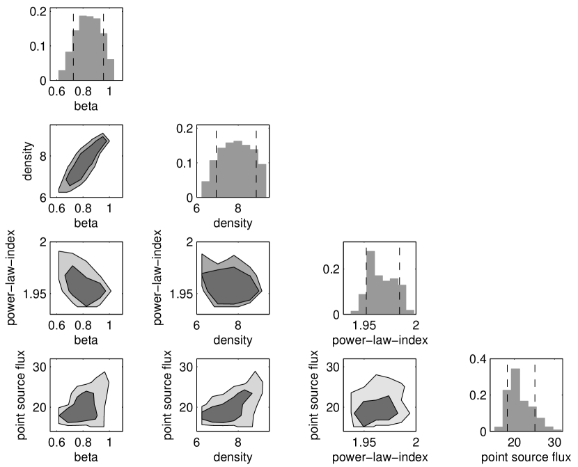
Figure 9: Same as Figure 5 for the spherical power-law model with an unresolved component. The absolute flux uncertainty is included. Marginalized posterior probability distributions for all four parameters (dust opacity spectral index $\beta$, density $\rho_{0}$ at 100 AU in the unit of 10^-18 g cm^-3, envelope density power-law index $p$, and point source flux density at 1 mm in the unit of mJy) are shown. In the histograms, the dashed vertical lines enclose 68% or 1 $\sigma$ confidence interval, with the expectation values and $\sigma$ listed in Table 3. The dark and light areas in the 2-D contour plots are the 68% and 95% confidence regions.

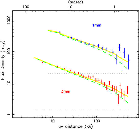
Figure 10: Same as Figure 6 but for the power-law envelope model plus an unresolved component. Error bars are statistical errors in the annuli-bins only. Observational flux density, averaged vectorially and binned in $u$-$v$ annuli around the source center, are shown by circles for the 1 mm data and asterisks for the 3 mm data. The model fit with the marginalized parameters is shown by solid lines, which includes two components: a power-law envelope (broken lines) and an unresolved disk (dotted lines).

Figure 11: Same as Figure 7 but for the power-law envelope model with an unresolved component. Comparison between 3 mm dust continuum data (upper row), model (middle row), and residuals (lower row) of L1157-mm in the image space.

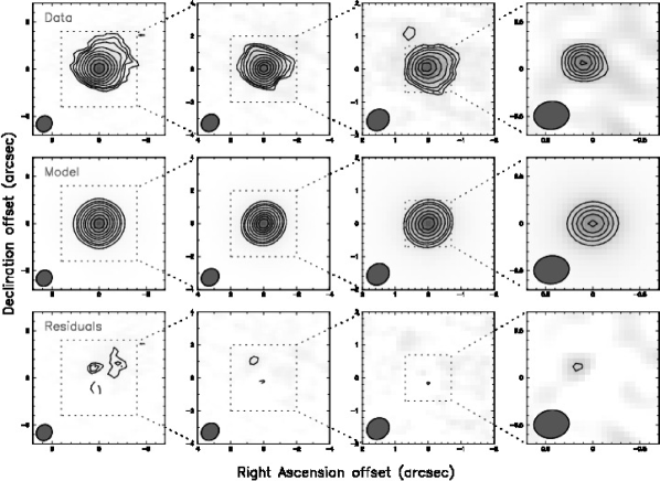
Figure 12: Same as Figure 8 but for the power-law envelope model with an unresolved component. Comparison between 1 mm dust continuum data (upper row), model (middle row), and residuals (lower row) of L1157-mm in the image space.

While a better fit with a smaller $\chi^{2}$ is achieved by the the power-law envelope model plus an unresolved component, the results are consistent with the results of the pure power-law envelope model presented in §4.1. The posterior-weighted mean of the density power-law index $p$ is slightly smaller than that of the pure power-law envelope model, due to the contribution of the point source flux. The dust opacity spectral index $\beta$ and density $\rho_{0}$ are consequently affected. With the added complexity of the model, larger uncertainties for the model parameters are obtained. In particular, the flux density of the unresolved component is not well constrained as it is not a necessary parameter. Nonetheless, the density index $p$ is still close to 2, so the inconsistency with the Shu model still exists (§4.1). The posterior-weighted mean of the unresolved flux is $\sim$2% compared to the total flux measured by single-dish observations (Gueth et al., 2003), and $\sim$11% of the flux measured by CARMA.

The flux density of the unresolved component can be converted to the upper limit of the embedded disk mass within the framework of the model. If we follow the empirical method of disk mass approximation in Looney et al. (2003) based on the disk modeling of HL Tau in Mundy et al. (1996), a disk of 0.05 M_⊙ at a distance of 140 pc is used as the standard candle for 100 mJy emission at 2.7 mm. As a result, our marginalized model gives a disk mass of 4.1 M_Jup. Alternatively, we can use a single-temperature optically thin source model to estimate the mass, that is,

$$M=F_{\nu}d^{2}/\kappa_{\nu}B_{\nu}(T)$$ (9)

(Hildebrand, 1983). Following Looney et al. (2000) with the assumptions of T = 60 K and $\kappa$=0.1($\nu$/1200 GHz) cm² g^-1 (dust+gas), the estimated disk mass is 3.6 M_Jup. Although these two methods of disk mass estimation give consistent results, the mass estimate is subject to the uncertainty of dust emissivity and temperature (see §5.3).

4.3 Rotating Collapse Model

Gravitational collapse of an envelope with uniform rotation has been studied in Ulrich (1976), Cassen & Moosman (1981), and Terebey, Shu, & Cassen (1984, hereafter the TSC model). The initial condition of the TSC model is a singular isothermal sphere, as in the Shu model. The non-zero angular momentum causes material to fall onto the midplane, following the streamline equation

$$\frac{r}{r_{c}}=\frac{\sin^{2}\theta_{0}}{1-\cos\theta/\cos\theta_{0}},$$ (10)

where $r_{c}$ is the centrifugal radius, $\theta$ is the angle from the rotation axis, and $\theta_{0}$ is the angle of the streamline at large $r$. A disk structure is expected inside the envelope with the density distribution

$$\rho=\frac{\dot{M}}{4\pi(GMr^{3})^{1/2}}(1+\frac{\cos\theta}{\cos\theta_{0}})^{-1/2}(\frac{\cos\theta}{\cos\theta_{0}}+\frac{2\cos^{2}\theta_{0}}{r/r_{c}})^{-1}.$$ (11)

We adopt the TSC model for the envelope fitting. The model parameters include: (a) the dust opacity spectral index $\beta$ as in Eq. (3), (b) the dust density $\rho_{0}$ at 100 AU, (c) the centrifugal radius $r_{c}$ of the TSC model in Eq. (10) and Eq. (11), and (d) a point source flux density (at 1 mm) to represent any unresolved component. The unresolved component is assumed to have the same dust properties as the envelope for scaling the 1 mm flux density to 3 mm. Besides that the TSC model implies an embedded disk, this point source flux density is required to obtain good fits with the TSC envelope; we were not able to obtain a fit with 90% confidence level with a zero unresolved flux.

The model parameters are investigated as in §4.1 and §4.2. Figure 13 shows the marginalized probability distributions of model parameters, and Table 4 lists the expectation values and uncertainties.

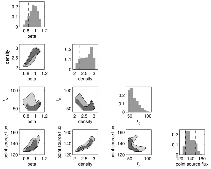
Figure 13: Same as Figure 5 but for the TSC model with an unresolved component. The absolute flux uncertainty is included. Marginalized posterior probability distributions for all four parameters (dust opacity spectral index $\beta$, density $\rho_{0}$ at 100 AU in the unit of 10^-18 g cm^-3, centrifugal radius $r_{c}$, and point source flux density at 1 mm in the unit of mJy) are shown. In the histograms, the dashed vertical lines enclose 68% or 1 $\sigma$ confidence interval, with the expectation values and $\sigma$ listed in Table 4. The dark and light areas in the 2-D contour plots are the 68% and 95% confidence regions.

Furthermore, visualization of the model-data comparison using the marginalized parameters is shown in both the visibility domain and image domain in Figure 14, Figure 15, and Figure 16

Table 4: TSC Model with an Unresolved Component

Parameter	Mean	Radius of the 68% confidence interval
		(statistical noise only)	(with flux uncertainty)
(1)	(2)	(3)	(4)
dust opacity spectral index $\beta$	0.96008	0.00022	0.10
density at 100 AU (in 10-18 g cm-3)	2.7203	0.0022	0.34
centrifugal radius $r_{c}$ (in AU)	44.9236	0.0016	14
unresolved 1 mm flux density (in mJy)	135.0764	0.0067	8.9

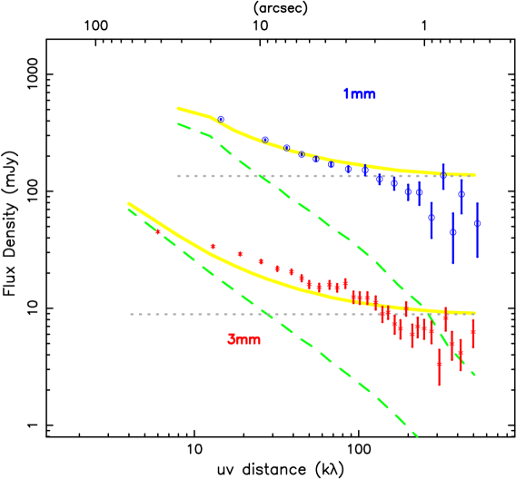
Figure 14: Same as Figure 10 but for the TSC envelope model plus an unresolved component. The total model fit (solid lines) includes two components: an envelope (broken lines) and an unresolved disk (dotted lines).

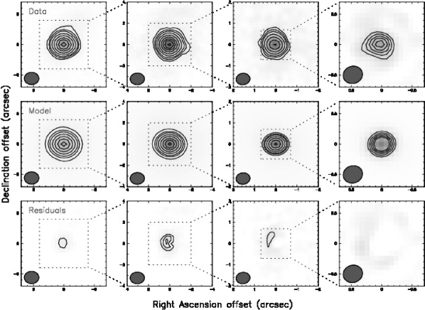
Figure 15: Same as Figure 7 but for the TSC model with an unresolved component. Comparison between 3 mm dust continuum data (upper row), model (middle row), and residuals (lower row) of L1157-mm in the image space.

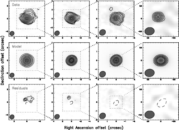
Figure 16: Same as Figure 8 but for the TSC model with an unresolved component. Comparison between 1 mm dust continuum data (upper row), model (middle row), and residuals (lower row) of L1157-mm in the image space.

The TSC model only fits the data with a bright point source component. In this case, the envelope contributes little flux towards the total dust continuum, and the unresolved disk component dominates the emission at both 1 mm and 3 mm, especially at long baselines (see Figure 14). While a rather shallow envelope model such as TSC is assumed, a strong small-scale component is required to fit the data. Similar results have also been seen in other studies (e.g., Terebey et al., 1993; Enoch et al., 2009). As discussed in §4.2, the unresolved flux density can be converted to the upper limit of disk mass. The posterior-weighted parameter implies an embedded disk of $\sim$25 M_Jup using either method in §4.2.

Although the best-fit model passes a chi-square hypothesis test (or the null hypothesis is rejected with 90% confidence), the TSC model does not fit the data as well as the power-law envelope model does. As seen in Figure 15 and Figure 16, the model does not subtract the data as cleanly as the power-law model does and leaves more residuals. In particular, residuals at 5 $\sigma$ level are seen in the 3 mm image (column 2 in Figure 15). A worse fit is also shown by the larger $\chi^{2}$, which will be examined in more detail in §5.1.

5 Discussion

5.1 Model Comparison

A model is just a simplification of the unknown reality, but we want to know which model provides a better approximation to all available data. In this section we apply model selection techniques and rank the models.

By applying Bayesian inference at the model level, one can use the Bayesian evidence for model selection. As discussed in Appendix B (Eq. (B1) and Eq. (B2)), the Bayesian evidence represents the probability of data given the model. It is marginalized over the full parameter space so the values of model parameters are not important, as opposed to parameter estimation for a particular model (§4). For comparing two competing models, the ratio of evidence, also known as the Bayes factor, represents posterior odds and can infer whether one model is preferred over the other (see Liddle, 2009, for a review).

However, an exact method to compute the Bayesian evidence needs to fully evaluate likelihood in the entire parameter space and is very computationally expensive. The posterior distribution sampled by MCMC (§4) peaks around the maximum posterior probability, and is not sufficient to calculate the Bayesian evidence. Approximation such as the use of information-theoretic methods is a good alternative approach for model selection (e.g., Liddle, 2007). For example, the Akaike information criterion (AIC, Akaike, 1974), derived using the Kullback-Leibler information (or K-L distance), is defined as

$$\textrm{AIC}\equiv-2\ln\mathcal{L}_{max}+2k,$$ (12)

where $\mathcal{L}_{max}$ is the maximum likelihood and $k$ is the number of model parameters. AIC provides a simple measure of how good the model approximates the information contained by the data, and a smaller value implies less information is lost and hence a better model. Detailed derivation and statistical implications can be found in Burnham & Anderson (2002). A second-order AIC, or AIC corrected, is suggested for small-sample bias adjustment as in

$$\textrm{AIC}_{c}=\textrm{AIC}+\frac{2k(k+1)}{N-k-1},$$ (13)

where $N$ is the number of data points. But in our case, $N\gg k$ so AIC and AIC_c converge. On the other hand, the Bayesian information criterion (BIC, Schwarz, 1978), defined as

$$\textrm{BIC}\equiv-2\ln\mathcal{L}_{max}+k\ln N,$$ (14)

is an approximation based on the Bayesian evidence ratio (also see Liddle, 2004).

A good model seeks for balance between goodness of fit and model simplicity. To obtain a better fit to the data or a smaller $\chi^{2}$, one may increase the model complexity with more parameters, but unnecessary use of parameters and over-fitting should be discouraged. The tradeoff is also seen in Eq. (12) and Eq. (14). As the best model minimizes AIC and BIC, smaller $\chi^{2}$ decreases the first term but extra parameters increase the second term. Model complexity in terms of the number of parameters is penalized in either AIC or BIC.

In this study, we evaluate AIC_c and BIC for all models. Because either AIC_c or BIC is on a relative scale, only the differences instead of actual values are meaningful (Burnham & Anderson, 2002). Results are listed in Table 5, where the model with the smallest value is preferred. As AIC_c and BIC suggest different ranking between the pure power-law envelope model and the power-law envelope plus an unresolved component, we do not make an inference between them. However, the results show a large positive $\Delta$AIC_c and $\Delta$BIC for the TSC model, implying that the power-law envelope model (either with or without the unresolved component) is decisively preferred against the TSC model plus an unresolved component.

Table 5: Model Comparison

Model	# of parameters	$\chi^{2}_{min}$ = $\Delta$(-2 ln$\mathcal{L}_{max}$)	$\Delta$AICc	$\Delta$BIC
(1)	(2)	(3)	(4)	(5)
Power-law envelope	3	9613473.1	1.9	0
Power-law envelope + an unresolved component	4	9613469.2	0	12.2
TSC envelope + an unresolved component	4	9615698.7	2229.5	2241.7

The model selection results are consistent with the a posteriori check presented in §4. Compared to either the pure power-law envelope model or the power-law envelope plus an unresolved component, considerable residuals are seen in the image domain for the TSC model plus an unresolved component.

5.2 Grain Growth

As mentioned in §3.3, dust properties are characterized by the opacity spectral index $\beta$ in our modeling. Depending on the environment, $\beta$ typically varies between 0 and 2. While $\beta\sim$ 2 implies small grains as in the interstellar medium, a smaller $\beta$ is usually found in many YSOs (e.g., Natta et al., 2007). Decrease of $\beta$ can be caused by many factors, such as change of composition or grain geometry, but is usually associated with change of grain size distribution (e.g., Krügel & Siebenmorgen, 1994). The $\beta$ value can be an evolutionary indicator of the dust grains in YSOs, as small grains in YSOs grow through coagulation, and eventually form planets if conditions allow. Nevertheless, Miyake & Nakagawa (1993) studied the size effect and showed that the observed decrease of $\beta$ in disk regions can be explained by the growth of grain size without change of chemical composition. If the grains in a dense region are composed of the same materials as in the interstellar grains, the maximum grain size is expected to be larger than 3 mm to explain the observational results of $\beta$ $\lesssim 1$ (Draine, 2006). Grain growth has been the most widely accepted explanation for the small $\beta$ found in protoplanetary disks (e.g., Beckwith et al., 2000; Draine, 2006).

In the three envelope models presented in §4, the posterior-weighted mean of $\beta$ range from 0.84 to 0.96. The absolute flux calibration dominates the uncertainty of $\beta$ estimation, resulting in a systematic uncertainty of $\sim$0.1. Still, $\beta$ being significantly smaller than the interstellar value is indicated. Our $\beta$ estimate for L1157-mm is in agreement with the samples of Class 0 YSOs in Jørgensen et al. (2007), Kwon et al. (2009), and Shirley et al. (2011b). The result implies that dust grains in L1157-mm, and arguably most Class 0 YSOs, have gone through some grain growth to at least millimeter size from the initial interstellar grains. However, when exactly dust grains start to grow during the protostellar evolution is uncertain. For example, Ricci et al. (2010a) compared $\beta$ of YSOs with their evolutionary ages and did not find apparent trend or difference in $\beta$ for YSOs in different evolutionary stages.

As a uniform dust grain property is adopted in our simple dust model, our estimate of $\beta$ represents the grain property in the whole system, including disk and envelope. Depending on the assumed envelope model, the embedded disk can contribute a significant fraction of flux. Compared to grains in the envelope, grains in the disk are expected to be larger in size as an initial step of planet formation. Therefore, a smaller $\beta$ is expected in the disk than in the envelope. Besides, grain properties are likely to vary across the envelope, as has been observationally suggested for some Class 0 sources (e.g., Chandler & Richer, 2000; Kwon et al., 2009). Since our L1157-mm data are consistent with a single $\beta$ value accross the envelope, the radial dependence of $\beta$ or a disk with a different $\beta$ is not modeled in this study; to address the dust property change in YSOs requires a more complex model.

5.3 The Earliest Circumstellar Disks

Circumstellar disks form as a physical consequence of angular momentum conservation when protostars accrete materials from their surrounding envelopes. These planet-forming pre-main-sequence disks have been observed and studied extensively (e.g., see the reviews of Williams & Cieza, 2011). In particular, disk evolution from early Class 0 to Class I stage is interesting as it is the phase during which most mass accretion occurs. The mass and size of the disk grow rapidly as the system evolves and depend on the rotation rate and the magnetic field strength of the background cloud, as well as the detailed mechanisms of angular momentum redistribution (e.g., Terebey et al., 1984; Basu, 1998; Machida & Matsumoto, 2011; Dapp et al., 2012).

While the mass and size of these youngest disks are essential to reveal the early process of disk formation, observing them is, however, not straightforward. In addition to the limitations of observational resolution and sensitivity, these disks are deeply embedded in their natal envelopes; probing them usually relies on indirect methods. For example, detection of water and methanol lines in Class 0 protostars can constrain the embedded circumstellar disks as the emission probably originates from the warm shocked layer of the disk-envelope interface, while different scenarios may not be ruled out (e.g., Goldsmith et al., 1999; Velusamy et al., 2002; Watson et al., 2007; Jørgensen & van Dishoeck, 2010). Near-infrared scattered light images, showing a dark lane along the edge-on disk, have also been used to infer the embedded disk structure (Tobin et al., 2010).

Another way to probe these youngest disks in embedded YSOs is through observations of dust continuum with a two-component model. The millimeter data consists of data continuum from both the disk and the envelope; with accurate modeling of the envelope, the circumstellar disk comopnent can be separated. In other words, the disk component is measured as the residual emission with the envelope contribution subtracted (e.g., Keene & Masson, 1990; Looney et al., 2003; Harvey et al., 2003; Jørgensen et al., 2005; Chiang et al., 2008; Enoch et al., 2009). This method avoids the complexity of chemical effects, but requires the use of a theoretical envelope model.

Using a two-component model, attributing the entire unresolved flux to be from the embedded disk, and following the mass estimation in Looney et al. (2000) and Looney et al. (2003), we derive the disk mass to be $\sim$4 M_Jup assuming a power-law envelope, or $\sim$25 M_Jup assuming a TSC envelope. Note that this mass estimate is an upper limit valid only within the framework of the models, and is highly dependent of the assumed envelope structure, dust opacity, disk temperature, and optical depth. For the envelope structure, we have shown that the power-law envelope model is preferred against the TSC model. But a large uncertainty still exists. For example, if instead we adopt a different dust opacity $\kappa$=0.015($\nu$/300 GHz) cm² g^-1 (dust+gas) and a single temperature of 30 K, as used in Greaves & Rice (2011), the disk mass is $\sim$13 M_Jup assuming the power-law envelope model. Our deduced disk mass is low compared to the estimate in Greaves & Rice (2011), where a disk mass of 80 M_Jup is obtained for L1157. Although Eq. (9) is also used in Greaves & Rice (2011), they assume the compact emission at 2″ is solely from the disk and no envelope subtraction is done, which possibly causes the differences in the estimated disk mass.

On the other hand, an empirical method that measures the small-scale flux at baseline $\sim$50 k$\lambda$ has also been used to estimate the unresolved disk component in embedded YSOs (Jørgensen et al., 2009; Enoch et al., 2011). This is based on the presumption that the envelope contributes little flux $\gtrsim$50 k$\lambda$. The 1 mm flux density of L1157-mm is around 200 mJy at 50 k$\lambda$, implying a disk mass of $\sim$174 M_Jup using $\kappa_{1.3mm}$=0.009 cm² g^-1 (Enoch et al., 2011). The estimated disk mass is comparable to other Class 0 sources in Enoch et al. (2011) and lighter than those in Jørgensen et al. (2009), but much heavier than our disk mass estimate using a two-component model. The empirical method of Jørgensen et al. (2009) and Enoch et al. (2011) seems to over-estimate the disk component in L1157-mm; one reason is that the flux density drops significantly longward of 50 k$\lambda$ (Figure 1) so the flux from the unresolved disk is apparently lower than 200 mJy. In addition, a relatively shallow envelope profile is assumed in either study (power-law of 1.5 in Jørgensen et al. 2009 and TSC in Enoch et al. 2011), and the assumed envelope structure considerably affect the flux ratio from envelope and disk.

Since our observations do not resolve the circumstellar disk, we can put an upper limit on the disk size for L1157-mm. Assuming a distance of 250 pc, the upper limit of the disk radius is $\sim$40 AU. This is consistent with the theoretical scenario of Dapp et al. (2012) in which Class 0 disks are small. This size constraint for L1157-mm is also consistent with those in other Class 0 YSOs. For example, no disks are detected for a sample of 5 Class 0 objects in Maury et al. (2010) with a resolution down to 0.3″, corresponding to a size scale of 42-75 AU, and the embedded disk at the edge-on Class 0 YSO VLA 1623A is constrained to be smaller than 50 AU in radius (Ward-Thompson et al., 2011). On the contrary, the disk embedded in the edge-on Class 0 YSO L1527 has been resolved by 7 mm VLA observations in Loinard et al. (2002); the disk structure is also seen with SMA and CARMA observations (Tobin et al. 2012). The size of Class 0 disks is comparable to or smaller than the size of older circumstellar disks (e.g., Eisner et al., 2005; Andrews et al., 2009; Vicente & Alves, 2005), but no clear trend can be inferred at this point.

6 Summary

1. Multi-configuration CARMA observations of the edge-on Class 0 YSO L1157-mm are presented. In our dust continuum data at both 1 mm and 3 mm, a nearly spherical circumstellar envelope is seen at the size scale of $\sim$10² to $\sim$10³ AU. No circumstellar disk on the small scale is resolved.

2. Radiative transfer modeling is performed to compare the interferometric data with the theoretical envelope models. A power-law envelope and a TSC envelope are considered. We add an unresolved component to represent the embedded disk. Bayesian inference is employed for parameter estimation. The absolute amplitude uncertainty, resulting from the flux calibration of the data reduction process, plays a critical role in parameter errors.

3. A density index $p\sim$ 2 is suggested for the power-law envelope, consistent with the results in Looney et al. (2003) for a larger sample of Class 0 YSOs. An unphysical young age is suggested if the Shu model is applied strictly. The data can be fitted by a pure power-law envelope without a compact emission from the embedded disk component.

4. The dust grain properties of the envelope are studied through the dust opacity spectral index $\beta$. The result $\beta\sim$ 0.9 is significantly smaller than the $\beta$ value in the interstellar medium, implying that grain growth has already started in L1157-mm.

5. The unresolved disk component is constrained to be $\lesssim$40 AU in radius and $\lesssim$4-25 M_Jup in mass. However, the mass estimate of the embedded disk component heavily relies on the assumed envelope model as well as the assumed disk characteristics. For example, a shallow envelope, such as the TSC model with a density power-law index $p\sim$ 1.5 in the outer region, requires a strong point source flux from the unresolved disk, while a steep envelope with $p\sim$ 2 can fit the observational data without an embedded disk.

6. Different envelope models are compared using an information-theoretic approach. The results prefer the power-law envelope model against the TSC model, which is also shown in the a posteriori check in the image domain.

7. This is the first study that utilizes the Bayesian techniques and model selection to consider multiple envelope models and make statistical inference for embedded YSOs. Future observations, especially high-resolution ALMA observations, will resolve the transition zone between the envelope and the disk, and further constrain the structures of Class 0 YSOs.

Appendix A Error Estimate of the Approximate Dust Opacity Spectral Index

In the optically thin limit and the Rayleigh-Jeans regime, the dust opacity spectral index $\beta_{thin}$ can be approximated using the flux density at two wavelengths. In this appendix we discuss the error propagation from the observational uncertainty to the deduced $\beta_{thin}$ value. Let $F_{1}$ and $F_{2}$ be the flux density at frequencies $\nu_{1}$ and $\nu_{2}$, $\beta_{thin}$ can be expressed as in Eq. (4):

$$\beta_{thin}=\frac{\ln F_{1}-\ln F_{2}}{\ln\nu_{1}-\ln\nu_{2}}-2.$$ (A1)

Assuming $F_{1}$ and $F_{2}$ are indenpendent variables with standard deviations $\sigma_{1}$ and $\sigma_{2}$, the standard error propagation gives

$$\sigma_{\beta_{thin}}^{2}=\left|\frac{\partial\beta_{thin}}{\partial F_{1}}\right|^{2}\sigma_{1}^{2}+\left|\frac{\partial\beta_{thin}}{\partial F_{2}}\right|^{2}\sigma_{2}^{2}.$$ (A2)

Taking the partial derivative of Eq. (A1), we obtain

$$\frac{\partial\beta_{thin}}{\partial F_{1}}=\frac{1}{(\ln\nu_{1}-\ln\nu_{2})F_{1}}$$ (A3)

and

$$\frac{\partial\beta_{thin}}{\partial F_{2}}=-\frac{1}{(\ln\nu_{1}-\ln\nu_{2})F_{2}}.$$ (A4)

Replacing Eq. (A2) using Eq. (A3) and Eq. (A4), the uncertainty of the derived $\beta_{thin}$ is then

$$\sigma_{\beta_{thin}}^{2}=\left(\frac{1}{\ln\nu_{1}-\ln\nu_{2}}\right)^{2}\left(\frac{\sigma_{1}^{2}}{F_{1}^{2}}+\frac{\sigma_{2}^{2}}{F_{2}^{2}}\right).$$ (A5)

Using Eq. (A5) and assuming the absolute flux error can be represented as a Gaussian noise with a standard deviation of 10%, that is, $\sigma_{1}=0.1F_{1}$ and $\sigma_{2}=0.1F_{2}$, the uncertainty of $\beta_{thin}$ is $\sim$0.15 for our data at 229 and 91 GHz. Note that here the error is assumed be normally distributed, different from the flat prior assumed in §4.

Appendix B Fitting Technique and Statistical Inference

In this appendix we give a brief introduction to Bayesian inference, as opposed to frequentist statistics. Also, we describe our technical procedure to characterize model parameters and their uncertainty.

The main concept of Bayesian inference is to incorporate prior knowledge on the hypothesis. Also, information is represented in terms of a probability density function (PDF) in parameter space. Mathematically, given the observed data, the posterior probability of model parameters can be specified by the Bayes’ theorem

$$P(x|D,M)=\frac{P(D|x,M)P(x|M)}{P(D|M)}$$ (B1)

where $x$ stands for model parameters, $D$ stands for data, $M$ denotes a particular model with its model assumptions and other background information, $P(x|M)$ is the prior probability of model parameters $x$, $P(D|x,M)$ is the conditional probability or the likelihood of data given the model with parameter $x$, and $P(D|M)$ is the evidence or global likelihood. The evidence $P(D|M)$ is the net probability of the data given the model, as it sums the product of likelihood and prior over parameter space:

$$P(D|M)=\int P(D|x,M)P(x|M)dx.$$ (B2)

The evidence is independent of the parameter values and can be seen as a normalizing factor in Eq. (B1); therefore it is not important for parameter estimation of a single model. For the same reason, the model label $M$ is sometimes omitted when only one model is considered. However, evidence is useful for comparing multiple models (§5.1).

Whether to view a statistics problem with Bayesian or frequentist approach is under debate. The disputes are beyond the scope of this study and more discussions can be found in Loredo (1990, 1992). Nevertheless, in the case of a uniform prior, the method of using the posterior probability is equivalent to maximum likelihood estimate as far as identifying the best-fit parameter values is concerned. As for full parameter estimation including estimating the parameter errors, different approaches are adopted for Bayesians and frequentists, and will be discussed later.

The likelihood of data given the model is characterized by $\chi^{2}$ (as defined in Eq. (7)) and $P(D|x)\sim$ exp$(-\chi^{2}(x,D)/2)$ with model parameter $x$ and observational data $D$. Therefore the most probable parameters with the maximum likelihood can be obtained by locating the global minimum of $\chi^{2}$. We use the Nelder-Mead simplex algorithm as implemented in MATLAB with bound constraints to search for the minimum. Besides fast convergence, this method does not evaluate function derivative, which suits our application because fewer modeling evaluations are required. Several starting points are used to look for several convergent minimums, and they are checked to be consistent with each other. This is to make sure that what is found is the global minimum, not a local minimum.

Once the best-fit parameter values are identified, efforts are made to characterize the uncertainty. The essence of parameter estimation is to characterize the reliability of an estimate on model parameters under the assumption that the best-fit model is correct. In other words, the best-fit model needs to show statistical significance based on a hypothesis test before any of the following parameter estimation can make sense. For example, in the standard Pearson’s chi-square hypothesis test, $\chi^{2}$ value of the model needs to be smaller than a critical value depending on the degrees of freedom to reject the null hypothesis. In the following we discuss two common methods of parameter estimation: (1) a frequentist approach to characterize $\Delta\chi^{2}$ and infer statistical significance, and (2) Markov chain Monte Carlo (MCMC) in the context of Bayesian inference.

The frequentist $\Delta\chi^{2}$ statistics has been suggested in Lampton et al. (1976) and Avni (1976), and summarized in Press et al. (2002). With the definition of $\Delta\chi^{2}(x)=\chi^{2}(x)-\chi^{2}(x_{best\mbox{-}fit})$, $\Delta\chi^{2}(x)$ is chi-square distributed with $p$ degrees of freedom, where $p$ is the number of fitted parameters or parameters of interest. Then the level of confidence can be estimated according to the chi-square distribution. Although it relies on the validity of the best-fit model, the exact value of $\chi^{2}(x_{best\mbox{-}fit})$ is not important for parameter estimation. The $\Delta\chi^{2}(x)$ statistics is independent of the Pearson’s chi-square test and $\chi^{2}(x)$ statistics, and focuses on the variation of $\chi^{2}(x)$ in parameter space $x$. A common way to illustrate the results is through iso-chi-square contours or hyper-surface in multi-dimensional parameter space as the confidence region. In the case that only partial parameters are of interest, the remaining nuisance parameters should be varied to minimize $\Delta\chi^{2}(x)$ instead of direct projections. (c.f. In Bayesian inference, the nuisance parameters are marginalized over.) For example, when only one parameter is of interest, $\Delta\chi^{2}(x)$ is distributed as a chi-square distribution with one degree of freedom. The 68% confidence interval corresponds to the region bounded by $\Delta\chi^{2}(x)=1$.

Despite the controversy over the flaws of applying this method with nonlinear models (Loredo, 1992), estimating $\Delta\chi^{2}(x)$ over a large parameter space can be computationally difficult. A grid on parameters or equivalent technique is required. The large number of evaluations usually makes this method impractical, especially when the number of parameters is large (Ford, 2005).

On the other hand, MCMC offers a very efficient way to estimate the posterior probability in Bayesian inference, compared to any other methods that require grid searching. Rather than minimizing on each grid point and probing the variation of $\chi^{2}(x)$, the posterior probability respect to parameters of interest is estimated through marginalization over all other parameters. For example, given a PDF $P(x_{1},x_{2}|D)$ where $x_{1}$ is the parameter of interest and $x_{2}$ is a nuisance parameter, the $x_{2}$ space is integrated over according to probability to obtain the marginalized PDF, as in

$$P(x_{1}|D)=\int P(x_{1},x_{2}|D)dx_{2}=\int P(x_{1}|x_{2},D)P(x_{2}|D)dx_{2}.$$ (B3)

At first glance, a straightforward marginalization can be very computationally extensive, similar to the necessity of a grid evaluation in frequentist methods. However, marginalized results can be obtained efficiently with MCMC. One of the reasons is that it searches the parameter space according to probability and the parameter space with low probability is less explored and sometimes not probed at all.

The Metropolis-Hastings algorithm of the MCMC method is utilized to construct the Markov chain. Markov chain is a sequence of parameter values representing the system and characterized by a transition probability that controls the random process from one state to another. The transition probability and the next state are only dependent of the current state, but not any previous states. Regardless of the starting state, the chain eventually converges to a stationary or equilibrium distribution according the PDF. We use the Metropolis-Hastings algorithm to draw the sample and construct the chain. This algorithm uses a proposal distribution $q(x^{\prime}|x)$, or the candidate transition probability distribution function, to generate a trial state $x^{\prime}$ based on the current state $x$. Then the proposed state is randomly accepted with the acceptance probability

$$\alpha(x^{\prime}|x)=\min\left[\frac{P(x^{\prime}|D)q(x|x^{\prime})}{P(x|D)q(x^{\prime}|x)},1\right],$$ (B4)

or otherwise rejected. The arrangement results in a transition probability

$$T(x^{\prime}|x)=q(x^{\prime}|x)\alpha(x^{\prime}|x)$$ (B5)

which is reversible ($\pi(x)T(x^{\prime}|x)=\pi(x^{\prime})T(x|x^{\prime})$, where $\pi(x)$ is the equilibrium probability at state $x$) and irreducible (possible to go from any state to any state). As introduced earlier, $P(x|D)$ is the posterior PDF given the observational data, and approximately proportional to exp$(-\chi^{2}(x,D)/2)$ with flat prior. Practically, $\chi^{2}(x,D)$ is evaluated at each proposed state change.

The Metropolis-Hastings algorithm assures that the chain converges to $P(x|D)$ as the sample number is large. The convergence rate is related to the choice of $q(x^{\prime}|x)$. A typical choice is a Gaussian function centered around x, that is,

$$q(x^{\prime}|x)=\frac{1}{\sqrt{2\pi w^{2}}}\exp\left(-\frac{(x^{\prime}-x)^{2}}{2w^{2}}\right)=q(x|x^{\prime}).$$ (B6)

The width of the Gaussian, specified by $w$, determines the trial step size. If the step size is too large, most trial states are rejected so the calculation becomes very inefficient; if the step size is too small, the chain behaves like a random walk and requires a long time to converge. An optimal acceptance rate is suggested to be around 0.23 for multi-dimensional parameter space (Gelman et al., 2004). The choice of a symmetric proposal distribution also reduces the acceptance probability into a simper form

$$\alpha(x^{\prime}|x)=\min\left[\frac{P(x^{\prime}|D)}{P(x|D)},1\right]=\min\left[\exp\left(\frac{\chi^{2}(x,D)-\chi^{2}(x^{\prime},D)}{2}\right),1\right].$$ (B7)

The posterior probability is obtained with a converged Markov chain, as its density of points in parameter space follows the posterior probability of the parameters. Marginalization is done through projecting the Markov chain to the space of parameters of interest. We estimate the 68% and 95% confidence limits and the corresponding standard deviation based on the simulated MCMC. Specifically, the 68% or 1 $\sigma$ confidence limit encloses 68% of accepted points along the Markov chain, and represents the region containing 68% of the total probability distribution. We also report the expectation value of each parameter, weighted by the posterior marginalized probability as in

$$\langle x_{i}\rangle=\int P(x_{i}|D)x_{i}dx_{i}=\frac{1}{N}\Sigma_{j}x_{i,j}$$ (B8)

where $j$ denotes the points in the Markov chain and $N$ is the total number of points. The expectation values from the marginalized distributions do not need to be identical to the parameters with the maximum likelihood, because we are projecting the values from a high dimensional distribution which may not be a multivariate Gaussian; however, they should be consistent.

References

- Adams (1991) Adams, F. C. 1991, ApJ, 382, 544
- Adams & Shu (1985) Adams, F. C. & Shu, F. H. 1985, ApJ, 296, 655
- Akaike (1974) Akaike, H. 1974, IEEE Transactions on Automatic Control, 19, 716
- Andrews et al. (2009) Andrews, S. M., Wilner, D. J., Hughes, A. M., Qi, C., & Dullemond, C. P. 2009, ApJ, 700, 1502
- Bachiller et al. (2001) Bachiller, R., Pérez Gutiérrez, M., Kumar, M. S. N., & Tafalla, M. 2001, A&A, 372, 899
- Basu (1998) Basu, S. 1998, ApJ, 509, 229
- Beckwith et al. (2000) Beckwith, S. V. W., Henning, T., & Nakagawa, Y. 2000, in Protostars and Planets IV, ed. V. Mannings, A. Boss, & S. S. Russell (Tucson: University of Arizona Press), 533
- Beckwith & Sargent (1991) Beckwith, S. V. W. & Sargent, A. I. 1991, ApJ, 381, 250
- Burnham & Anderson (2002) Burnham, K. P. & Anderson, D. R. 2002, Model Selection and Multimodel Inference: A Practical Information-Theoretic Approach, 2nd edn. (New York: Springer-Verlag)
- Cassen & Moosman (1981) Cassen, P. & Moosman, A. 1981, Icarus, 48, 353
- Chandler et al. (1998) Chandler, C. J., Barsony, M., & Moore, T. J. T. 1998, MNRAS, 299, 789
- Chandler et al. (1995) Chandler, C. J., Koerner, D. W., Sargent, A. I., & Wood, D. O. S. 1995, ApJ, 449, L139
- Chandler & Richer (2000) Chandler, C. J. & Richer, J. S. 2000, ApJ, 530, 851
- Chiang et al. (2008) Chiang, H.-F., Looney, L. W., Tassis, K., Mundy, L. G., & Mouschovias, T. C. 2008, ApJ, 680, 474
- Chiang et al. (2010) Chiang, H.-F., Looney, L. W., Tobin, J. J., & Hartmann, L. 2010, ApJ, 709, 470
- Choi et al. (1999) Choi, M., Panis, J.-F., & Evans, II, N. J. 1999, ApJS, 122, 519
- Dapp et al. (2012) Dapp, W. B., Basu, S., & Kunz, M. W. 2012, A&A, 541, A35
- Draine (2006) Draine, B. T. 2006, ApJ, 636, 1114
- Draine & Lee (1984) Draine, B. T. & Lee, H. M. 1984, ApJ, 285, 89
- Dullemond & Dominik (2004) Dullemond, C. P. & Dominik, C. 2004, A&A, 417, 159
- Eisner et al. (2005) Eisner, J. A., Hillenbrand, L. A., Carpenter, J. M., & Wolf, S. 2005, ApJ, 635, 396
- Enoch et al. (2011) Enoch, M. L., Corder, S., Duchêne, G., Bock, D. C., Bolatto, A. D., Culverhouse, T. L., Kwon, W., Lamb, J. W., Leitch, E. M., Marrone, D. P., Muchovej, S. J., Pérez, L. M., Scott, S. L., Teuben, P. J., Wright, M. C. H., & Zauderer, B. A. 2011, ApJS, 195, 21
- Enoch et al. (2009) Enoch, M. L., Corder, S., Dunham, M. M., & Duchêne, G. 2009, ApJ, 707, 103
- Evans et al. (2001) Evans, II, N. J., Rawlings, J. M. C., Shirley, Y. L., & Mundy, L. G. 2001, ApJ, 557, 193
- Ford (2005) Ford, E. B. 2005, AJ, 129, 1706
- Froebrich (2005) Froebrich, D. 2005, ApJS, 156, 169
- Galli & Shu (1993) Galli, D. & Shu, F. H. 1993, ApJ, 417, 220
- Gelman et al. (2004) Gelman, A., Carlin, J. B., S., S. H., & B., R. D. 2004, Bayesian data analysis, 2nd edn., Texts in statistical science (Boca Raton: Chapman & Hall/CRC)
- Goldsmith et al. (1999) Goldsmith, P. F., Langer, W. D., & Velusamy, T. 1999, ApJ, 519, L173
- Greaves & Rice (2011) Greaves, J. S. & Rice, W. K. M. 2011, MNRAS, 412, L88
- Gueth et al. (2003) Gueth, F., Bachiller, R., & Tafalla, M. 2003, A&A, 401, L5
- Gueth et al. (1996) Gueth, F., Guilloteau, S., & Bachiller, R. 1996, A&A, 307, 891
- Gueth et al. (1997) Gueth, F., Guilloteau, S., Dutrey, A., & Bachiller, R. 1997, A&A, 323, 943
- Harvey et al. (2003) Harvey, D. W. A., Wilner, D. J., Myers, P. C., Tafalla, M., & Mardones, D. 2003, ApJ, 583, 809
- Hennebelle & Fromang (2008) Hennebelle, P. & Fromang, S. 2008, A&A, 477, 9
- Hildebrand (1983) Hildebrand, R. H. 1983, QJRAS, 24, 267
- Hunter (1977) Hunter, C. 1977, ApJ, 218, 834
- Isella et al. (2009) Isella, A., Carpenter, J. M., & Sargent, A. I. 2009, ApJ, 701, 260
- Jørgensen et al. (2007) Jørgensen, J. K., Bourke, T. L., Myers, P. C., Di Francesco, J., van Dishoeck, E. F., Lee, C.-F., Ohashi, N., Schöier, F. L., Takakuwa, S., Wilner, D. J., & Zhang, Q. 2007, ApJ, 659, 479
- Jørgensen et al. (2005) Jørgensen, J. K., Bourke, T. L., Myers, P. C., Schöier, F. L., van Dishoeck, E. F., & Wilner, D. J. 2005, ApJ, 632, 973
- Jørgensen & van Dishoeck (2010) Jørgensen, J. K. & van Dishoeck, E. F. 2010, ApJ, 710, L72
- Jørgensen et al. (2009) Jørgensen, J. K., van Dishoeck, E. F., Visser, R., Bourke, T. L., Wilner, D. J., Lommen, D., Hogerheijde, M. R., & Myers, P. C. 2009, A&A, 507, 861
- Keene & Masson (1990) Keene, J. & Masson, C. R. 1990, ApJ, 355, 635
- Krügel & Siebenmorgen (1994) Krügel, E. & Siebenmorgen, R. 1994, A&A, 288, 929
- Kun (1998) Kun, M. 1998, ApJS, 115, 59
- Kun et al. (2008) Kun, M., Kiss, Z. T., & Balog, Z. 2008, Star Forming Regions in Cepheus (Astronomical Society of the Pacific, Edited by Bo Reipurth), 136
- Kwon et al. (2011) Kwon, W., Looney, L. W., & Mundy, L. G. 2011, ApJ, 741, 3
- Kwon et al. (2009) Kwon, W., Looney, L. W., Mundy, L. G., Chiang, H.-F., & Kemball, A. J. 2009, ApJ, 696, 841
- Larson (1969) Larson, R. B. 1969, MNRAS, 145, 271
- Lay et al. (1995) Lay, O. P., Carlstrom, J. E., & Hills, R. E. 1995, ApJ, 452, L73
- Liddle (2004) Liddle, A. R. 2004, MNRAS, 351, L49
- Liddle (2007) —. 2007, MNRAS, 377, L74
- Liddle (2009) —. 2009, Annual Review of Nuclear and Particle Science, 59, 95
- Loinard et al. (2002) Loinard, L., Rodríguez, L. F., D’Alessio, P., Wilner, D. J., & Ho, P. T. P. 2002, ApJ, 581, L109
- Lommen et al. (2007) Lommen, D., Wright, C. M., Maddison, S. T., Jørgensen, J. K., Bourke, T. L., van Dishoeck, E. F., Hughes, A., Wilner, D. J., Burton, M., & van Langevelde, H. J. 2007, A&A, 462, 211
- Looney et al. (2000) Looney, L. W., Mundy, L. G., & Welch, W. J. 2000, ApJ, 529, 477
- Looney et al. (2003) —. 2003, ApJ, 592, 255
- Looney et al. (2007) Looney, L. W., Tobin, J. J., & Kwon, W. 2007, ApJ, 670, L131
- Loredo (1990) Loredo, T. J. 1990, in Maximum-Entropy and Bayesian Methods, ed. P. Fougere (Dordrecht: Kluwer Academic Publishers), 81–142
- Loredo (1992) Loredo, T. J. 1992, in Statistical Challenges in Modern Astronomy, ed. E. D. Feigelson & G. J. Babu, 275–306
- Machida & Matsumoto (2011) Machida, M. N. & Matsumoto, T. 2011, MNRAS, 413, 2767
- Masunaga & Inutsuka (2000) Masunaga, H. & Inutsuka, S.-i. 2000, ApJ, 531, 350
- Mathis et al. (1977) Mathis, J. S., Rumpl, W., & Nordsieck, K. H. 1977, ApJ, 217, 425
- Maury et al. (2010) Maury, A. J., André, P., Hennebelle, P., Motte, F., Stamatellos, D., Bate, M., Belloche, A., Duchêne, G., & Whitworth, A. 2010, A&A, 512, A40
- Meehan et al. (1998) Meehan, L. S. G., Wilking, B. A., Claussen, M. J., Mundy, L. G., & Wootten, A. 1998, AJ, 115, 1599
- Miyake & Nakagawa (1993) Miyake, K. & Nakagawa, Y. 1993, Icarus, 106, 20
- Moreno & Guilloteau (2002) Moreno, R. & Guilloteau, S. 2002, An Amplitude Calibration Strategy for ALMA, ALMA Memo 372, ALMA
- Mundy et al. (1996) Mundy, L. G., Looney, L. W., Erickson, W., Grossman, A., Welch, W. J., Forster, J. R., Wright, M. C. H., Plambeck, R. L., Lugten, J., & Thornton, D. D. 1996, ApJ, 464, L169
- Natta et al. (2007) Natta, A., Testi, L., Calvet, N., Henning, T., Waters, R., & Wilner, D. 2007, in Protostars and Planets V, ed. B. Reipurth, D. Jewitt, & K. Keil (Tucson: University of Arizona Press), 767–781
- Nisini et al. (2010) Nisini, B., Benedettini, M., Codella, C., Giannini, T., Liseau, R., Neufeld, D., Tafalla, M., van Dishoeck, E. F., Bachiller, R., Baudry, A., Benz, A. O., Bergin, E., Bjerkeli, P., Blake, G., Bontemps, S., Braine, J., Bruderer, S., Caselli, P., Cernicharo, J., Daniel, F., Encrenaz, P., di Giorgio, A. M., Dominik, C., Doty, S., Fich, M., Fuente, A., Goicoechea, J. R., de Graauw, T., Helmich, F., Herczeg, G., Herpin, F., Hogerheijde, M., Jacq, T., Johnstone, D., Jørgensen, J., Kaufman, M., Kristensen, L., Larsson, B., Lis, D., Marseille, M., McCoey, C., Melnick, G., Olberg, M., Parise, B., Pearson, J., Plume, R., Risacher, C., Santiago, J., Saraceno, P., Shipman, R., van Kempen, T. A., Visser, R., Viti, S., Wampfler, S., Wyrowski, F., van der Tak, F., Yıldız, U. A., Delforge, B., Desbat, J., Hatch, W. A., Péron, I., Schieder, R., Stern, J. A., Teyssier, D., & Whyborn, N. 2010, A&A, 518, L120
- Ossenkopf & Henning (1994) Ossenkopf, V. & Henning, T. 1994, A&A, 291, 943
- Penston (1969) Penston, M. V. 1969, MNRAS, 144, 425
- Pérez et al. (2010) Pérez, L. M., Lamb, J. W., Woody, D. P., Carpenter, J. M., Zauderer, B. A., Isella, A., Bock, D. C., Bolatto, A. D., Carlstrom, J., Culverhouse, T. L., Joy, M., Kwon, W., Leitch, E. M., Marrone, D. P., Muchovej, S. J., Plambeck, R. L., Scott, S. L., Teuben, P. J., & Wright, M. C. H. 2010, ApJ, 724, 493
- Ricci et al. (2010a) Ricci, L., Testi, L., Natta, A., & Brooks, K. J. 2010a, A&A, 521, A66
- Ricci et al. (2010b) Ricci, L., Testi, L., Natta, A., Neri, R., Cabrit, S., & Herczeg, G. J. 2010b, A&A, 512, A15
- Robitaille et al. (2007) Robitaille, T. P., Whitney, B. A., Indebetouw, R., & Wood, K. 2007, ApJS, 169, 328
- Rodmann et al. (2006) Rodmann, J., Henning, T., Chandler, C. J., Mundy, L. G., & Wilner, D. J. 2006, A&A, 446, 211
- Sault et al. (1995) Sault, R. J., Teuben, P. J., & Wright, M. C. H. 1995, in Astronomical Society of the Pacific Conference Series, Vol. 77, Astronomical Data Analysis Software and Systems IV, ed. R. A. Shaw, H. E. Payne, & J. J. E. Hayes, 433
- Schnee et al. (2010) Schnee, S., Enoch, M., Noriega-Crespo, A., Sayers, J., Terebey, S., Caselli, P., Foster, J., Goodman, A., Kauffmann, J., Padgett, D., Rebull, L., Sargent, A., & Shetty, R. 2010, ApJ, 708, 127
- Schwarz (1978) Schwarz, G. 1978, Annals of Statistics, 6, 461
- Shirley et al. (2011a) Shirley, Y. L., Huard, T. L., Pontoppidan, K. M., Wilner, D. J., Stutz, A. M., Bieging, J. H., & Evans, II, N. J. 2011a, ApJ, 728, 143
- Shirley et al. (2011b) Shirley, Y. L., Mason, B. S., Mangum, J. G., Bolin, D. E., Devlin, M. J., Dicker, S. R., & Korngut, P. M. 2011b, AJ, 141, 39
- Shirley et al. (2005) Shirley, Y. L., Nordhaus, M. K., Grcevich, J. M., Evans, II, N. J., Rawlings, J. M. C., & Tatematsu, K. 2005, ApJ, 632, 982
- Shu (1977) Shu, F. H. 1977, ApJ, 214, 488
- Spergel et al. (2007) Spergel, D. N., Bean, R., Doré, O., Nolta, M. R., Bennett, C. L., Dunkley, J., Hinshaw, G., Jarosik, N., Komatsu, E., Page, L., Peiris, H. V., Verde, L., Halpern, M., Hill, R. S., Kogut, A., Limon, M., Meyer, S. S., Odegard, N., Tucker, G. S., Weiland, J. L., Wollack, E., & Wright, E. L. 2007, ApJS, 170, 377
- Straizys et al. (1992) Straizys, V., Cernis, K., Kazlauskas, A., & Meistas, E. 1992, Baltic Astronomy, 1, 149
- Tassis & Mouschovias (2005) Tassis, K. & Mouschovias, T. Ch. 2005, ApJ, 618, 769
- Terebey et al. (1993) Terebey, S., Chandler, C. J., & Andre, P. 1993, ApJ, 414, 759
- Terebey et al. (1984) Terebey, S., Shu, F. H., & Cassen, P. 1984, ApJ, 286, 529
- Tobin et al. (2011) Tobin, J. J., Hartmann, L., Chiang, H.-F., Looney, L. W., Bergin, E. A., Chandler, C. J., Masqué, J. M., Maret, S., & Heitsch, F. 2011, ApJ, 740, 45
- Tobin et al. (2010) Tobin, J. J., Hartmann, L., & Loinard, L. 2010, ApJ, 722, L12
- Ulrich (1976) Ulrich, R. K. 1976, ApJ, 210, 377
- van der Tak et al. (1999) van der Tak, F. F. S., van Dishoeck, E. F., Evans, II, N. J., Bakker, E. J., & Blake, G. A. 1999, ApJ, 522, 991
- Velusamy et al. (2002) Velusamy, T., Langer, W. D., & Goldsmith, P. F. 2002, ApJ, 565, L43
- Vicente & Alves (2005) Vicente, S. M. & Alves, J. 2005, A&A, 441, 195
- Vorobyov & Basu (2005) Vorobyov, E. I. & Basu, S. 2005, MNRAS, 360, 675
- Ward-Thompson et al. (2011) Ward-Thompson, D., Kirk, J. M., Greaves, J. S., & André, P. 2011, MNRAS, 415, 2812
- Watson et al. (2007) Watson, D. M., Bohac, C. J., Hull, C., Forrest, W. J., Furlan, E., Najita, J., Calvet, N., D’Alessio, P., Hartmann, L., Sargent, B., Green, J. D., Kim, K. H., & Houck, J. R. 2007, Nature, 448, 1026
- Whitney et al. (2003) Whitney, B. A., Wood, K., Bjorkman, J. E., & Wolff, M. J. 2003, ApJ, 591, 1049
- Whitworth & Summers (1985) Whitworth, A. & Summers, D. 1985, MNRAS, 214, 1
- Williams & Cieza (2011) Williams, J. P. & Cieza, L. A. 2011, ARA&A, 49, 67