Turbulent mixing driven by mean-flow shear and internal gravity waves in oceans and atmospheres

Abstract

This study starts with balances deduced by Baumert and Peters (2004, 2005) from results of stratified-shear experiments made in channels and wind tunnels by Itsweire (1984) and Rohr and Van Atta (1987), and of free-decay experiments in a resting stratified tank by Dickey and Mellor (1980). Using a modification of Canuto’s (2002) ideas on turbulence and waves, these balances are merged with an (internal) gravity-wave energy balance presented for the open ocean by Gregg (1989), without mean-flow shear. The latter was augmented by a linear (viscous) friction term. Gregg’s wave-energy source is interpreted on its long-wave spectral end as internal tides, topography, large-scale wind, and atmospheric low-pressure actions. In addition, internal eigen waves, generated by mean-flow shear, and the aging of the wave field from a virginal (linear) into a saturated state are taken into account. Wave packets and turbulence are treated as particles (vortices, packets) by ensemble kinetics so that the loss terms in all three balances have quadratic form. Following a proposal by Peters (2008), the mixing efficiency of purely wave-generated turbulence is treated as a universal constant, as well as the turbulent Prandtl number under neutral conditions. It is shown that: (i) in the wind tunnel, eigen waves are switched off, (ii) due to remotely generated long waves or other non-local energy sources, coexistence equilibria of turbulence and waves are stable even at Richardson numbers as high as $10^{3}$; (iii) the three-equation system is compatible with geophysically shielded settings like certain stratified laboratory flows. The agreement with a huge body of observations surprises. Gregg’s (1989) wave-model component and the a.m. universal constants taken apart, the equations contain only one additional dimensionless parameter for the eigen-wave closure, estimated as $Y\approx 1.35.$

Baumert Turbulence by shear & waves .. 35pc H. Z. Baumert, IAMARIS, Bei den Mühren 69A,
D-20457 Hamburg, Germany (baumert@iamaris.org) Report on the SHEWAMIX project, Grant N62909-10-1-7050, ONR-Global.

1 Introduction

1.1 General

In geophysical flows, turbulence is ubiquitous. Today turbulent engineering flows may already be simulated using DNS, i.e. fully resolving scales down to the smallest ones, provided they are large compared with molecular cluster scales. However, for ocean and atmospheric flows this will remain impossible even in the foreseeable future. Here particularly the dominating stably stratified flows, i.e. all forms of coexistence of turbulence and internal waves, represent a specific observational and theoretical challenge. Without a better understanding of the fundamental physics of these processes all our regional to global models of weather and climate remain incomplete.

Oceanic, atmospheric and stellar turbulence has challenged a number of prominent scientists and research groups since long, in the recent decade namely Woods (2002), Galperin et al. (2007), Canuto et al. (2008), and Zilitinkevich et al. (2008), also Kantha and Carniel (2009). They all emphasized a major contradiction between observational experience and existing theories:

• For controlled stratified shear flows in the laboratory exists undoubtly a critical gradient Richardson number of $R_{g}^{b}\leq{\cal O}(\hbox{$\,{}^{1}\!/_{4}$})$ above which turbulence dies out (Itsweire, 1984; Itsweire et al., 1986; Rohr and Van Atta, 1987; Rohr et al., 1987; Rohr et al., 1988a, b; Van Atta, 1999). Also in the field the qualitative and strongly (but not totally) limiting role of $R_{g}^{b}$ is without doubt (Peters et al., 1988) and became specifically visible with the advent of Lagrangian floaters in the Lagrangian time spectra of turbulence and wave-like fluctuations where $\Omega=N$ marks a sharp divide: to the left a flat wave spectrum, to the right a Kolmogorov time spectrum (D’Asaro and Lien, 2000a, b). Also the existing theories (Richardson, 1923; Miles, 1961; Howard, 1961; Hazel, 1972; Thorpe, 1973, Abarbanel et al., 1984; Baumert and Peters, 2004) point all into the same direction.

• Geophysical flows are reported to exhibit not always, but more than often significant stable turbulence levels and mixing capabilities at $R_{g}\gg\hbox{$\,{}^{1}\!/_{4}$}$ (Peters et al., 1988; Canuto, 2002; Poulos et al., 2002; Nakamura and Mahrt, 2005; Grachev et al., 2005, 2006). Also Peters and Baumert (2007) report problems in validating a $K$-$\varepsilon$ turbulence closure against comprehensive estuarine microstructure measurements in the Hudson river. For tidal phases with weak shear the observed turbulence levels exceeded the model values by 2 to 3 orders of magnitude. The dynamic time lag of the turbulent state variables in the M₂ tide (about one hour, see Baumert and Radach, 1992) can be excluded as a source of the deviations because the model naturally contains this effect.

The text below makes an attempt to resolve the sketched contradiction using ideas of Woods (2002 and literature cited therein) and Canuto (2002) regarding the role of waves and billow turbulence. We identify internal gravity waves (so far neglected in most other studies) as the potentially responsible phenomenon.

For a better understanding of the language used in this text we first introduce notational conventions and then continue with an overview of major physical processes within the world of stratified shear turbulence and internal gravity waves.

Below, we always means the author and the dear reader in a dialogue.

1.2 Setup and notation

For simplicity we focus on a simple non-trivial situation, a spatially one-dimensional “channel” flow with velocity component $U$ in horizontal ($x$) direction, with variation of $U$ along the vertical, $z$ (pointing upwards), and with Eulerian density and icopycnal coordinate fluctuations.

The decomposition of our flow field into mean and fluctuations reads as follows:

$$U(z,t) = \langle U\rangle+\tilde{u}(z,t)+u^{\prime}(z,t)\,,$$ (1)

$$W(z,t) = \langle W\rangle+\tilde{w}(z,t)+w^{\prime}(z,t)\,.$$ (2)

Variables with tilde are small-scale short-wave components, present only under stratified conditions. Primed variables denote turbulent fluctuations. Both fluctuating components vanish in the mean.

The turbulent kinetic energy, TKE or $\cal K$, is defined as follows,

$${\cal K}=\frac{1}{2}\langle u^{\prime 2}+v^{\prime 2}+w^{\prime 2}\rangle.$$ (3)

A wave’s total energy, $\cal E$, is the sum of potential, $\langle N^{2}\,\tilde{\zeta}^{2}\rangle/2$, and kinetic energy, $\langle\tilde{u}^{2}+\tilde{w}^{2}\rangle/2$ (Gill, 1982):

$${\cal E}=\frac{1}{2}\langle\tilde{u}^{2}+\tilde{w}^{2}+N^{2}\,\tilde{\zeta}^{2}\rangle.$$ (4)

Here $\tilde{u}$ points into the direction of wave propagation so that in a plane wave $\tilde{v}=0$. Average $\langle.\rangle$ is taken at least over one wave period which “by definition” is longer than the characteristic turbulent time scale. In the following the dimensionless gradient Richardson number, $R_{g}$, plays a central role. In a stratified shear flow as above, shear is given by

$$\langle S\rangle=\frac{\partial\langle U\rangle}{\partial z}\,,$$ (5)

while stratification is characterized by the Brunt-Väisälä frequency squared,

$$\langle N^{2}\rangle=-\frac{g}{\langle\rho\rangle}\,\frac{d\langle\rho\rangle}{dz}.$$ (6)

$\langle\rho\rangle$ is the background density field.

The gradient Richardson number, $R_{g}$, characterizes the dimensionless ratio of the two aspects, shear and stratification:

$$R_{g}=\langle N^{2}\rangle/\langle S\rangle^{2}\,.$$ (7)

Below the averaging operators are mostly omitted for brevity of notation. But fluctuations are consequently labeled either by tilde (wave-like) or prime (turbulent).

Based on $R_{g}$, under controlled laboratory conditions where the linear eigen waves leave the experimental site before quadratic saturation and a feed back into the TKE pool can happen (wind tunnel of Van Atta), the following hydrodynamic regimes for horizontally homogeneous flows are found (Baumert and Peters, 2004, 2005):

• $R_{g}\leq R_{g}^{a}\equiv 0$: unstable and neutral stratification,
  convective turbulence, no internal waves at all.

• $0\equiv R_{g}^{a}<R_{g}<R_{g}^{b}\equiv\hbox{$\,{}^{1}\!/_{4}$}$: stable stratification, shear-dominated growing turbulence, coexistence of turbulence and internal waves.

• $\hbox{$\,{}^{1}\!/_{4}$}\equiv R_{g}^{b}<R_{g}<R_{g}^{c}\equiv\hbox{$\,{}^{1}\!/_{2}$}$: stable stratification,
  wave-dominated decaying turbulence, coexistence of turbulence and internal waves.

• $\hbox{$\,{}^{1}\!/_{2}$}\equiv R_{g}^{c}<R_{g}$: stable stratification, no coexistence of turbulence and waves, waves-only regime.

Under those conditions the turbulent Prandtl number $\sigma$ is (Baumert and Peters, 2004, 2005)

$$\sigma=\frac{\mu}{\nu}=\frac{\sigma_{0}}{1-(N/\Omega)^{2}}$$ (8)

The above values for the critical numbers $R_{g}^{a},R_{g}^{b}$ and $R_{g}^{c}$ hold for the asymptotic case $Re\rightarrow\infty$.

The situation is different if we leave the laboratory wind tunnel and consider the open ocean, stratified rivers or the stably stratified atmosphere where turbulence is not only locally generated through local mean-flow shear but also through the action of space-filling (non-local) spectra of internal gravity waves (IGWs). These are generated e.g. by tidal forces, possibly at remote places, arriving at our point of interest along various pathways.

2 Major physical interactions in stably stratified oceans and atmospheres

Fig. 1 schematically presents the major interactions between the energies of mean and fluctuating motion components. Fig. 2 does the same for r.m.s. vorticity and turbulent viscosity, $\nu$. The latter connects $\cal K$ and $\Omega$ with the mean flow through the so-called Kolmogorov-Prandtl relation in the following form (Baumert and Peters, 2004, Baumert, 2012):

$$\nu={{\cal K}}/{\pi\,\Omega}\,.$$ (9)

The TKE dissipation rate, $\varepsilon$, transforming TKE into heat, is defined as (Baumert and Peters, 2004, Baumert, 2012)

$$\varepsilon={{\cal K}\,\Omega}/{\pi}=\nu\,\Omega^{2}\,.$$ (10)

The buoyancy flux, $B$, transforming TKE into background potential energy, $PE_{b}$, may be expressed using the eddy diffusivity, $\mu$, as follows,

$$B=-\frac{g}{\langle\,\rho\rangle}\langle w^{\prime}\,\rho^{\prime}\rangle=\mu\,N^{2}\,,$$ (11)

where $\mu$ is related with the eddy viscosity $\nu$ through $\sigma$, the turbulent Prandtl number function:

$$\mu=\nu/\sigma\,\quad\quad\mbox{or}\quad\quad\sigma=\nu/\mu\,.$$ (12)

Finally, the molecular heat flux, $\Phi_{i}$, transforms internal energy into background potential energy, $PE_{b}$.

There is further the rate $\Pi$, which transforms the energy of internal tides and wind-generated large-scale internal motions over a long chain of various friction-poor wave-wave interactions into short-wave internal-wave energy, and there is the rate $\tilde{P}$, which transforms the energy of internal-waves spectra into TKE, mainly by breaking (a shot noise process), and to a low degree by wave shear.

The mean-flow shear, $S$, controls TKE production through $P-\Psi$ and internal-wave generation through $\Psi$. In the (conventional) neutrally stratified case, $N^{2}=0$, the total loss term in the mean-flow kinetic-energy balance (MKE) is $-P$, which is at the same time the only source of small-scale energy:

$$P=\nu\,S^{2}\,.$$ (13)

But for $N^{2}>0$ small-scale energy means the sum of turbulence and waves, $P=(P-\Psi)+\Psi.$

The shear governs not only TKE and IGW production but also the generation of r.m.s. vorticity. But vorticity is also influenced by short internal-gravity waves through the term $\tilde{S}$: in the shearless IGW-dissipation case (e.g. Gregg, 1989) we have also vorticity generation.

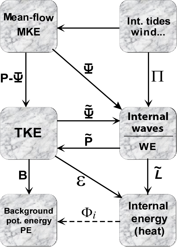
Figure 1: Interaction of major forms of fluid-mechanical energy in stratified oceanic, atmospheric or stellar shear flows. $\Psi$ is the flux of eigen-wave energy mentioned in the text. $\Pi$ is the energy flow which corresponds to remotely generated waves. The wind tunnel allows to cut off the flux $\tilde{P}$ from the the wave-energy to the TKE pool because the wave spectrum cannot reach a saturated state. In the long-term equilibrium holds $\tilde{P}=(1-f)(\Psi+\Pi)$ where $f$ is the fraction of direct wave dissipation and tends to zero if the wave spectrum approaches saturation. $f$ may become relevant for short wave ages.

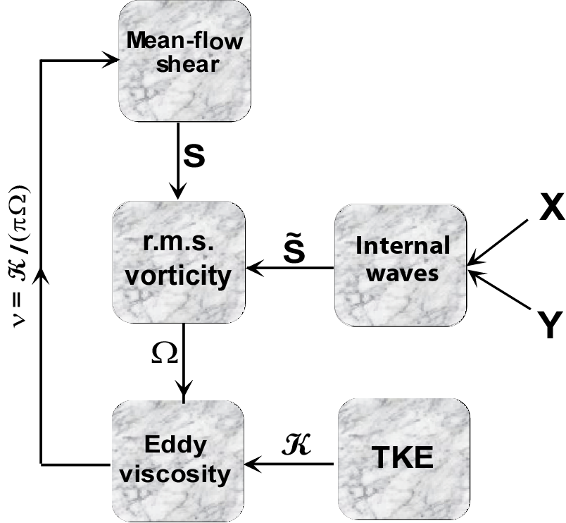
Figure 2: Interaction of major vorticity-controlling motion components in stratified oceanic and atmospheric shear flows. The r.m.s. vorticity $\Omega$ is governed by the mean-flow shear, $S$, and a wave-induced pseudo shear, $\tilde{S}$. The latter is controlled by eigen waves ($Y$) and remotely generated long waves ($X$). For details see text.

When we use the word energy in the present context, we mostly mean for brevity TKE ($\cal K$), i.e. turbulent kinetic energy. If we talk here about vorticity we similarly mean for brevity the r.m.s. turbulent vorticity. For its detailed mechanical interpretation we refer to Baumert (2012).

The precise meaning of $\Omega$ is actually the module of the vorticity frequency. The module of the vorticity itself, $\omega$, is $\omega=2\,\pi\,\Omega$. The enstrophy is ${\omega^{2}}/{2}$.

3 Balances for small-scale motions

Before we start to write down transport equations for primary variables we first discuss their nature and their balances. For this aim we look again at Fig. 1 and there namely on the two boxes in the middle row with the names TKE and Internal waves.

The left box, TKE, is fed by two components: by mean-flow shear in the form of $P-\Psi$, and by internal-wave breaking, $\tilde{P}$, see (15) below. But it generates heat by $\varepsilon$ via (10), exports buoyancy $B$ via (11), and generates by $\tilde{\Psi}$ in the course of aging and subsequent collapse short internal waves, when its time scale approaches the internal-wave period (Baumert and Peters, 2005).

Turbulence collapsing into waves is an event mostly bound to certain special conditions (e.g. Dickey and Mellor, 1980; D’Asaro and Lien, 2000a, b). Under smooth and almost-equilibrium conditions the TKE may collapse and generate waves which then after aging saturate and feed their energy back into the TKE pool, as part of $\tilde{P}$. In the following $\tilde{\Psi}$ is therefore mostly neglected.

The right box, Internal waves, is fed by three components: by large-scale wave sources, $\Pi$, by the rate of eigen-wave generation, $\Psi$, and by the collapse rate discussed already above and neglected further below. This box further exhibits two relevant losses: the linear wave friction, $\tilde{L}$,

$$\tilde{L}=c_{1}\,{\cal E}\,,$$ (14)

and the quadratic wave friction, $\tilde{P}$,

$$\tilde{P}=c_{2}\,{\cal E}^{2}\,.$$ (15)

The latter is mainly caused by wave breaking and dominates the wave-energy balance, but not completely. The loss term (14) and (15) follows arguments developed by Gregg (1989) which we augment as follows.

From a purely theoretical point of view the phenomenon of wave breaking tells us nothing about its kinetics. It is the processes before breaking occurs which form the bottleneck. If we accept the idea that not only vortices (actually: vortex-dipole filaments, see Baumert, 2012) are particles which move in space until collision, then the interpretation of wave-energy dynamics in terms of particle dynamics does not come as a surprise, in particular in view of the billow turbulence discussed by Woods (2002).

Due to the general particle-wave dualism of field theories, which is a well established concept in classical continuum mechanics, also wave packets can be treated as particles moving with their group velocity until collision. After collision they either move ahead, or change their paths, or, with low probability, their energy is dissipated by breaking in dissipative patches (billows). In contrast to vortex kinetics, here the probabilities are not symmetric. In both cases (vortex dipoles and wave packets) the collision events are highly intermittent.

Besides its phenomenological basis, the quadratic term in (15) might therefore have deeper roots or at least analogies in the kinetics of reactive particle “gases” or molecular reactions in fluids where particle-collision probabilities follow the product of their spatial densities. For collisions between particles of same kind, the quadratic collision term is thus a logical consequence.

Fig. 2 shows the major feedback loop between the small-scale motions and the mean flow which eventually smoothes the flow through the turbulent viscosity. The central left box, r.m.s. vorticity, is fed by two components: by the mean-flow shear, $S$, and by the internal-wave field through the pseudo shear, $\tilde{S}$. The vorticity $\Omega$ itself controls together with the TKE $\cal K$ the turbulent viscosity via (9) which eventually smoothes the flow.

The spectral signatures of shear-generated fluctuations and wave-wave interactions differ qualitatively. While shear influences vorticity directly by prescribing a time scale $\propto S^{-1}$, the long-wave sources ($\Pi$) of IGW spectra do it more indirectly via a longer chain of wave-wave interactions cascading down to critical frequencies around $N$. This implies that each of the two mechanisms needs “his” closure.

For conditions of homogeneous shear, stratification and wave fields the above three balances can be so far formulated as follows (compare with Figs. 1 and 2 ):

$$\frac{d\Omega}{dt} = \frac{1}{\pi}\left(\frac{S^{2}}{2}-\Omega^{2}+\tilde{S}^{2}\right),$$ (16)

$$\frac{d{\cal K}}{dt} = (P-\Psi)-B-\varepsilon+\tilde{P},$$ (17)

$$\frac{d\cal E}{dt} = (\Pi+\Psi)-\tilde{L}-\tilde{P}.$$ (18)

With the exception of $\Pi$, all variables in (16, 17, 18) have purely local character.

In (17) we used the relation

$$B+\Psi=\nu\,N^{2}/\sigma_{0}\,,$$ (19)

derived and discussed in greater detail by Baumert and Peters (2004, 2005). Here $\sigma_{0}=\hbox{$\,{}^{1}\!/_{2}$}$ is the value of the turbulent Prandtl number function $\sigma$ for the case of neutral stratification ($R_{g}=0$ or $\Omega\rightarrow\infty$). With (8) we have

$$\Psi=\frac{\varepsilon}{\sigma_{0}}\,\left(\frac{N}{\Omega}\right)^{4}.$$ (20)

Note that the system (16 – 18) is not one of the common three-equation models used in traditional turbulence modeling. The focus of this modeling branch is directed on higher and higher orders of the closure equations, e.g. equations for second and third moments and so forth, all derived from the Navier-Stokes equation.

In later sections we will see that the system (16 – 18) is dynamically stiff. Under spatially homogeneous conditions well-defined steady-state solutions exist, but perturbations of this state are connected with very different characteristic relaxation times of the systems components. In particular, $\Omega$ is the component relaxing fastest into what we call structural equilibrium. The TKE ($\cal K$) relaxes significantly slower into a new state while the wave energy, $\cal E$, relaxes extremely slowly. The wave-energy pool needs a longer spin-up time because the flux of shear-generated wave energy, $\Psi$, consists of random linear wave packets which simply need time “to meet and break”, of course by chance.

Figure 3: Linear wave packet, hypothetically generated by shear. Breaking occurs by chance superpositions and results in dissipative patches or billows.

For later use we introduce here the “viscous fraction” $f$ of the total energy loss of the wave pool towards the heat pool,

$$f=\frac{\tilde{L}}{\tilde{L}+\tilde{P}}$$ (21)

with the obvious property

$$f+\frac{\tilde{P}}{\tilde{L}+\tilde{P}}=1.$$ (22)

The fraction $1-f$ describes a “wave age”, i.e. the relative wave-energy loss into the TKE pool. Clearly,

$$0\leq f<1.$$ (23)

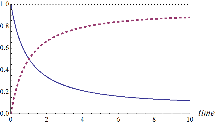
Figure 4: Solid: laminar (linear) loss fraction of wave energy in the course of saturation, $f(t)=\tilde{L}(t)/(\tilde{L}(t)+\tilde{P}(t))$; dashed: “wave age”, $1-f(t)$.

We note in passing that the steady state is not the only dynamically invariant state of TKE and waves. Also the state of exponential evolution (Van Atta, 1999) in wind tunnels belongs to this class. This state, taken as a reference, has also the property that perturbations relax back towards reference.

In our present situation where we deal with relaxation times orders of magnitudes apart, the use of the so-called Tikhonov principle seems to be helpful. It means to concentrate on processes with moderate relaxation times. (16) is so fast that it can be taken as being always in structural equilibrium. (18) is so slow that its time derivative is small compared with the source and sink terms at the right-hand side and can be neglected. We are thus left with only one differential and two algebraic equations. However, in the case of very stiff algebraic equations it is sometimes more useful to apply the method of non-stationary embedding. Here it would mean to re-establish the character of (16) and (18) as differential equations and to seek the stationary solution via relaxation to the stationary state.

4 Special cases

Below we discuss some special cases of our general system(16 –18): the neutrally stratified case ($N=0$), the stratified ($N^{2}>0$) but geophysically shielded ($\Pi=0$) case, and the stably stratified wind tunnel.

4.1 Neutral stratification, $N=0$

Homogeneous shear means constant shear along the horizontal and vertical axes. The assumption $N=0$ means neutral stratification. Internal gravity waves of any kind are not supported by the fluid so that all terms in (18) vanish, together with this equation. Further, the terms $\Psi,\;\;\Pi$, $\tilde{P}$, $\tilde{S}$ are zero such that eventually (16, 17) look as follows:

$$\frac{d\Omega}{dt} = \frac{1}{\pi}\left(\frac{S^{2}}{2}-\Omega^{2}\right),$$ (24)

$$\frac{d{\cal K}}{dt} = P-\varepsilon.$$ (25)

These equations correspond to a clear mechanistic interpretation of turbulence as dipole chaos in the sense of a two-fluid approach (excitons in form of quasi-rigid vortex tubes made of inviscid fluid, and the materially identical inviscid but not excited fluid between the tubes) derived by Baumert (2005 – 2012). As a byproduct, this theory gives von Karman’s number as $\kappa=1/\sqrt{2\,\pi}=0.399$.

4.2 Stable stratification, $N^{2}>0$, $\Pi=0$

Here we mean stratified shear flows under idealized laboratory conditions where the role of tides and external geophysical influences are excluded, i.e. $\Pi=0$, which implies also $\tilde{S}=0$, to be discussed later. These conditions are called below “geophysically shielded”.

Homogeneity means here constant $N^{2}$ and $S^{2}$ in the horizontal plane and on the vertical axis, which is not easy to realize in a laboratory. But on a simplistic theoretical level we can get some insight when we consider only the stationary system (16, 17, 18). The vorticity balance gives trivially $\Omega^{2}=S^{2}/2$ and is therefore omitted for brevity. It remains the following:

$$0 = P-\Psi-B-\varepsilon+\tilde{P},$$ (26)

$$0 = \Psi-\tilde{L}-\tilde{P}\,.$$ (27)

We neglect the linear molecular friction $\tilde{L}$, rewrite (27) to get $\tilde{P}\approx\Psi$; wie insert this into (26) and get the following:

$$P\approx B+\varepsilon\,.$$ (28)

Remarkably, $\Psi$ cancels out of (26, 27) so that finally the oceanographer’s standard balance formulation (28) is obtained. We come back to this point later.

In the past experiments with stratified wind tunnels gave deep insights into the nature of the turbulence-wave interactions (Rohr et al., 1988; Van Atta, 1999; Baumert and Peters 2004, 2005). However, they do not support relation (28). This is the contradiction we mentioned in the Introduction and will be discussed next.

4.3 The stratified wind tunnel, $\Pi=0$, $R_{g}>0$

4.3.1 The system.

This important case is an example of strong horizontal inhomogeneity and non-equilibrium conditions. In the entrance facility of the tunnel the forced flow passes a fine grid which leaves an initial high-frequency short-wave turbulence and internal-wave signature in a locally homogeneous fluid body of limited size. We consider this fluid body as moving with the mean flow in a plug-flow sense. The small-scale properties then evolve during the trip within the fluid body along the homogeneously sheared and stratified tunnel until its end, where the body leaves the tunnel, including its small-scale properties. Typically an exponential evolution of TKE is observed along the longitudinal axis, either exponential growth or exponential decay (Van Atta, 1999). The waves were not recorded but it must be hypothesized that they did reach saturation level.

This situation is artificial. In a natural hydrodynamic system the growth of turbulence is limited because it would somewhere begin to reduce its own source (shear) by mixing the mean flow (see Fig. 2) so that an equilibrium will sooner or later be reached, corresponding to the large-scale energy input to the flow. But this feedback from the turbulence-wave system to the mean-flow system takes time and the travel time through the tunnel is too short.

Exactly this sort of decoupling of processes is what the tunnel experimentalists aim at. They wish in particular to cut off the feedback $\tilde{P}$ from shear-generated wave-energy into TKE, as it contaminates the clear and simple picture. In other words, they want to see the naked interrelations in stratified shear turbulence as studied already by Richardson (1920), Howard (1961) and Miles (1961). Those three authors neglected shear-generated waves and their subsequent feedback as a result of spectral saturation.

4.3.2 Advection-dispersion-reaction (ADR) and the plug-flow concept.

At a first glance the sheared flow of a stratified wind tunnel seems to represent a major problem for detailed analyses. However, the Taylor-Aris theory of shear dispersion (Taylor, 1953; Aris, 1956; Baumert, 1973; Fischer et al., 1979) allows to compute an effective longitudinal dispersion coefficient, $D_{L}$, and to cast the transport equations corresponding to (16, 17, 18) in the following general form of an advection-dispersion-reaction equation:

$$\frac{\partial Y}{\partial t}+\frac{\partial}{\partial x}\left(\langle U\rangle\,Y-D_{L}\,\frac{\partial Y}{\partial x}\right)=-Y/\hat{\tau}.$$ (29)

Here $Y$ is a placeholder for the variables $\Omega$, $\cal K$, and $\cal E$, and $\hat{\tau}$ is an effective time constant of a hypothetically decaying (or growing, when $\hat{\tau}<0$) variable $Y$.

As long as the Peclet number of the problem, $Pe=\left|\langle U\rangle^{2}\hat{\tau}/(4\,D_{L})\right|\gg 1$, it can be shown (e.g. Baumert, 1973) that the stationary form of (29, with ${\partial Y}/{\partial t}=0$) can be simplified into a so-called plug-flow description:

$$\langle U\rangle\,\frac{dY}{dx}\approx-Y/\hat{\tau}.$$ (30)

In a wind tunnel this concept is a useful approximation because the velocity $\langle U\rangle$ and thus the above similarity number are typically high enough. In a stationary plug-flow sense we thus have :

$$\langle U\rangle\frac{\partial\Omega}{\partial x} = \frac{1}{\pi}\left(\frac{S^{2}}{2}-\Omega^{2}\right),$$ (31)

$$\langle U\rangle\frac{\partial\cal K}{\partial x} = P-\Psi-B-\varepsilon+\tilde{P},$$ (32)

$$\langle U\rangle\frac{\partial\cal E}{\partial x} = \Psi-\tilde{L}-\tilde{P}.$$ (33)

Now we introduce the dimensionless travel-time coordinate along the wind-tunnel axis,

$$\hat{t}=x\cdot S/\langle U\rangle.$$ (34)

We further introduce dimensionless variables via

$$\hat{\Omega} = \Omega\,\sqrt{2}/S\,,$$ (35)

$$\hat{\cal K} = {\cal K}/{\cal K}_{0}\,,$$ (36)

$$\hat{\cal E} = {\cal E}/{\cal E}_{0}\,.$$ (37)

Here ${\cal K}_{0}$ and ${\cal E}_{0}$ are the initial conditions so that
$\hat{\cal K}_{t=0}=\hat{\cal E}_{t=0}=1$. Due to the initiation of the flow by the grid the vorticity typically begins with high initial values, $\hat{\Omega}_{t=0}\gg 1$.

4.3.3 General case.

The above conventions allow to rewrite the transport equations (31, 32, 33) with some algebra in dimensionless form:

$$\frac{d\hat{\Omega}}{d\hat{t}} = \frac{1}{2\,\pi}\left(1-\hat{\Omega}^{2}\right),$$ (38)

$$\frac{d\hat{\cal K}}{d\hat{t}} = \left(2-\frac{2R_{g}}{\sigma_{0}}-\hat{\Omega}^{2}\right)\frac{\hat{\cal K}}{\pi\,\hat{\Omega}\,\sqrt{2}}+\frac{\tilde{P}}{S\cdot{\cal K}_{0}},$$ (39)

$$\frac{d\hat{\cal E}}{d\hat{t}} = \frac{{\cal K}_{0}}{{\cal E}_{0}}\left(\frac{\sqrt{8}}{\pi\,\sigma_{0}}\,R_{g}^{2}\;\frac{\hat{\cal K}}{\hat{\Omega}^{3}}-\frac{\tilde{P}}{S\cdot{\cal K}_{0}}\right).$$ (40)

Here we neglected the linear molecular friction term $\tilde{L}=c_{1}\,\cal E$ and replaced according to (19) $\Psi$ with $\nu\,N^{2}/\sigma_{0}-B$. For $B$ we used (11) and (12).

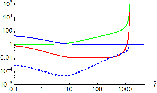
Figure 5: Wind-tunnel turbulence-waves model in dimensionless variables. $\hat{\Omega}$ (solid blue) converges soon ($\hat{t}\approx 10$) to its structural-equilibrium value, $\hat{\Omega}_{\infty}=1$. $\hat{K}$ (solid red) goes through a minimum and starts at $\hat{t}\approx 10$ a phase of exponential growth. $\hat{\cal E}$ (solid green) rests long time close to its initial condition $\hat{\cal E}_{0}=1$ and enters at $\hat{t}\approx 10$ into a phase of exponential growth. The ratio $\tilde{P}/\Psi$ (dashed blue, $0<\tilde{P}/\Psi<1$) remains initially very small but jumps then around $\hat{t}\approx 1500$ to its asymptotic value $(\tilde{P}/\Psi)_{\infty}=1.$ In this example $R_{g}=0.16$, $\hat{\alpha}=10^{-6}$, and $\beta=1$. Notice the double-logarithmic character of the presentation.

We now abbreviate $\alpha={\cal E}_{0}/S$, $\beta={\cal E}_{0}/{\cal K}_{0}$ and $\hat{\alpha}=\alpha\times c_{2}$ so that

$$\frac{d\hat{\Omega}}{d\hat{t}} = \frac{1}{2\,\pi}\left(1-\hat{\Omega}^{2}\right),$$ (41)

$$\frac{d\hat{\cal K}}{d\hat{t}} = \left(2-\frac{2R_{g}}{\sigma_{0}}-\hat{\Omega}^{2}\right)\frac{\hat{\cal K}}{\pi\,\hat{\Omega}\,\sqrt{2}}+\hat{\alpha}\,\beta\,\hat{\cal E}^{2},$$ (42)

$$\frac{d\hat{\cal E}}{d\hat{t}} = \frac{1}{\beta}\left(\frac{\sqrt{8}}{\pi\,\sigma_{0}}\,R_{g}^{2}\;\frac{\hat{\cal K}}{\hat{\Omega}^{3}}-\,\hat{\alpha}\,\beta\,\hat{\cal E}^{2}\right).$$ (43)

According to Gregg (1989), in the ocean we have $c_{2}=7.4\times 10^{-5}$ s  m^-2. $\alpha$ and $c_{2}$ are the only parameters or variables in (41 – 43) which are not dimensionless. But the two appear only in form of the product $\hat{\alpha}=\alpha\times c_{2}$, which is again dimensionless and was already used in (42) and (43). To make an order of magnitude estimate of $\hat{\alpha}$ we take for $S$ the Garret-Munk value, $S_{GM}=0.0036$ s^-1, and $\hat{\cal E}\approx 10^{-4}$ m²s^-2. This gives a characteristic guess of $\hat{\alpha}\approx{\cal O}(10^{-6}$). This value was used to compute the data in Fig. 5.

The system (41 – 43) can be solved numerically by standard methods if its high stiffness is adequately taken into account. The first phase of the evolution based on (41 – 43) is shown in Fig. 5 where we may identify three regimes with two separating breakpoints. The first regime is the initialization or spin-up regime. The first breakpoint labels its end at $\hat{t}\approx 10$ and is associated with the transition into structural equilibrium. The second regime may be called the typical wind-tunnel regime (an artificially decoupled or naked turbulence-wave system in exponential growth, $\tilde{P}\approx 0$). Its end is labeled by the second breakpoint at $\hat{t}\approx 1500$. The third regime can be called a hyper-equilibrium regime characterized by $\tilde{P}=\Psi$ and exponential growth, too. Both exponential growth regimes exhibit the property

$$\frac{1}{\hat{K}}\frac{d\hat{K}}{d\hat{t}} = \mbox{constant}\,,$$ (44)

$$0 = \frac{d}{d\hat{t}}\left(\frac{1}{\hat{K}}\frac{d\hat{K}}{d\hat{t}}\right)\,.$$ (45)

We use for regime 3 the name hyper equilibrium because it has the condition $\tilde{P}=\Psi$ in common with the natural equilibrium (oceanographer’s regime) but differs with respect to the dynamic state: while in the natural case all first time derivatives vanish, in the hyper case they are constants $>0$, but the second derivatives vanish.

The simulations show that in an ideal stratified wind tunnel of infinite length the hyper-equilibrium regime can in principle be reached, e.g. for $\hat{t}\gg 1500$. But such a length can hardly be achieved in practice. Thus the most interesting and scientifically unique part in a stratified wind tunnel (or a salt-stratified channel flow) is the section between the lower and the upper breakpoint.

In a somewhat sloppy form we may summarize: the total travel time through the wind tunnel is too short for the shear-generated waves to develop a saturated spectrum which would almost equate the breaking term $\tilde{P}$ with the generation term $\Psi$.

5 Stably stratified natural shear flows: $R_{g}>0$, $\Pi>0,\tilde{S}^{2}>0$

We now come back to the system (16, 17, 18) and study its the TKE balance where the waves and the vorticity are assumed to stay in a steady state:

$$0 = S^{2}/2-\Omega^{2}+\tilde{S}^{2},$$ (46)

$$0 = \Pi+\Psi-\tilde{L}-\tilde{P}\,,$$ (47)

$$\frac{d\cal K}{dt} = P+\tilde{P}-\Psi-B-\varepsilon\,.$$ (48)

5.1 TKE balance and mixing efficiencies

The definition (21) allows now to rewrite the TKE balance (48) as follows,

$$\frac{d\cal K}{dt}=(1-f)\Pi+P-B-\varepsilon-f\,\Psi\,.$$ (49)

Shear and occasionally overturning waves are qualitatively different generation mechanisms with differing spectral signatures, differing mixing efficiencies and differing buoyancy fluxes. Both mechanisms are associated with buoyancy fluxes which add up (parallel circuitry??) to the total buoyancy flux $B$:

$$B = B^{\prime}+\tilde{B}\,.$$ (50)

The so-called mixing efficiency, $\Gamma$, is generally defined as $\Gamma=B/\varepsilon$. Due to the additive nature of $B=B^{\prime}+\tilde{B}$ also $\Gamma$ is additive:

$$\Gamma=\frac{B}{\varepsilon}\;=\frac{B^{\prime}+\tilde{B}}{\varepsilon}\;=\;\frac{B^{\prime}}{\varepsilon}+\frac{\tilde{B}}{\varepsilon}=\Gamma^{\prime}+\tilde{\Gamma}\,.$$ (51)

With these preliminaries we may rewrite (49) as follows:

$$\frac{d\cal K}{dt}=(1-f)\,\Pi+P-B^{\prime}-\tilde{B}-\varepsilon-f\,\Psi\,.$$ (52)

5.1.1 Mixing efficiency of purely shear-generated turbulence: $\Gamma^{\prime}=\Gamma^{\prime}(R_{g});\;\tilde{B}=0,\;\tilde{P}=0,\;\Pi=0,\;\tilde{S}^{2}=0.$

Using exclusively definitions like (10) and (8) given in the previous sections and subsections, we begin here to specify $B^{\prime}$ as follows:

$$B^{\prime}=\varepsilon\;\Gamma^{\prime}=\mu\,N^{2}=\frac{\nu}{\sigma}\,N^{2}=\frac{\nu}{\sigma_{0}}\left[1-\left(\frac{N}{\Omega}\right)^{2}\right].$$ (53)

We solve (53) for $\Gamma^{\prime}$ and get the following:

$$\Gamma^{\prime}=\frac{\nu}{\sigma}\,\frac{N^{2}}{\varepsilon}=\frac{1}{\sigma}\left(\frac{N}{\Omega}\right)^{2}=\frac{1}{\sigma_{0}}\left(\frac{N}{\Omega}\right)^{2}\left[1-\left(\frac{N}{\Omega}\right)^{2}\right].$$ (54)

In the pure shear-generated case, $\Pi=\tilde{S}=0$, we thus have $\Omega^{2}=S^{2}/2$, and with $R_{g}=N^{2}/S^{2}$ (54) rewrites as follows:

$$\Gamma^{\prime}=\frac{2}{\sigma_{0}}R_{g}\left(1-2\,R_{g}\right).$$ (55)

This function is presented in Fig. 6 and is well supported by observations as shown in an earlier study by Baumert and Peters (2004, 2005).

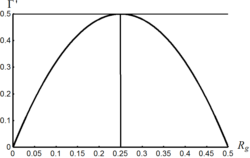
Figure 6: The mixing efficiency $\Gamma^{\prime}$ according to equation (55) for shear-generated turbulence.

5.1.2 Mixing efficiency of purely wave-generated turbulence: $\tilde{\Gamma}=\tilde{\Gamma}_{0}=0.2;\;P=\Psi=0,\;S=0.$

The mixing situation is qualitatively different in the case without mean-flow shear where turbulence is exclusively generated by wave spectra fed eventually by large-scale long-wave external sources. According to the state of the art (Osborne, 1980; Oakey, 1982; Gregg et al., 1986; Peters et al. 1988), the mixing efficiency may still be taken to be a universal constant, $\tilde{\Gamma}=\tilde{\Gamma}_{0}=0.2$. Clearly, in purely shear-generated turbulence a gradient-Richardson number is not available so that $\tilde{\Gamma}$ cannot be a function of it. Further, in this case this number is not even defined because the shear is zero.

5.2 The remote-wave closure and oceanographer’s balance: $P=\Psi=0,\;S=0,\;\Pi>0,\;\tilde{S}^{2}>0$

Here we will derive an approximate relation between the large-scale long-wave source of wave-generated turbulence (“remote waves”), $\Pi$, and the correspondingly induced component $\tilde{S}^{2}$ in the vorticity balance (46). We choose a flow without mean-flow shear, $S=0$ and $B^{\prime}=0$, such that, according to (46), $\Omega^{2}=\tilde{S}^{2}$. The TKE balance (52) reads in this case

$$\frac{d\cal K}{dt}=(1-f)\,\Pi-\tilde{B}-\varepsilon\,,$$ (56)

and in the steady state:

$$(1-f)\,\Pi=\tilde{B}+\varepsilon.$$ (57)

The remaining rate $f\,\Pi$ describes the linear or molecular energy loss of the wave field.

We replace $\tilde{B}$ with $\tilde{\Gamma}\,\varepsilon$ and get

$$(1-f)\,\Pi=\tilde{\gamma}\,\varepsilon=\tilde{\gamma}\,\nu\,\Omega^{2}=\tilde{\gamma}\,\nu\,\tilde{S}^{2}$$ (58)

so that the following is finally the closure of our problem:

$$\tilde{S}^{2}=\frac{(1-f)\,\Pi}{\tilde{\gamma}\,\nu}\,.$$ (59)

6 Natural coexistence equilibria

We consider now the general natural coexistence of waves and turbulence where $0\leq f<1$, $\Pi>0$, $P>0$ etc.

6.1 Vorticity

We insert the approximate closure relation (59) in the vorticity balance (46) and get with the abbreviation $\tilde{\gamma}=1+\tilde{\Gamma}$

$$\Omega^{2}=\frac{S^{2}}{2}+\frac{(1-f)\,\Pi}{\tilde{\gamma}\;\nu}\,.$$ (60)

For convenience reasons we introduce $\eta$ and choose for (60) the following presentation,

$$\eta=\frac{\Omega^{2}}{S^{2}}=\frac{1}{2}+\frac{X}{\tilde{\gamma}},$$ (61)

where for our convenience

$$X=(1-f)\,\frac{\Pi}{\nu\,S^{2}}=(1-f)\,\frac{\Pi}{P}.$$ (62)

6.2 TKE

Now we discuss the steady-state version of the general TKE balance (52):

$$(1-f)\,\Pi+P=B^{\prime}+\tilde{B}+\varepsilon+f\,\Psi\,.$$ (63)

According to our previous discussions, it may be written as follows:

$$(1-f)\,\Pi+\nu\,S^{2}=\frac{\nu}{\sigma}\,N^{2}+\tilde{\gamma}\,\varepsilon+\frac{f}{\sigma_{0}}\left(\frac{N}{\Omega}\right)^{4}\varepsilon.$$ (64)

We rewrite this equation identically as

$$(1-f)\,\Pi+\nu\,S^{2}=\frac{\nu}{\sigma}\,N^{2}+\left[\tilde{\gamma}+\,\frac{f}{\sigma_{0}}\left(\frac{N}{\Omega}\right)^{4}\right]\nu\,\Omega^{2},$$ (65)

and divide both sides of (65) by $\nu\,S^{2}$ to get with (62)

$$1+X=\frac{R_{g}}{\sigma}+\left[\tilde{\gamma}+\,\frac{f}{\sigma_{0}}\left(\frac{N}{\Omega}\right)^{4}\right]\eta\;.$$ (66)

We now expand $(N/\Omega)^{4}$ into $(N/S)^{4}/(\Omega/S)^{4}=R_{g}^{2}/\eta^{2}$, replace $\eta$ with (61) and get finally

$$\left(\frac{N}{\Omega}\right)^{4}=\left(\frac{R_{g}}{\eta}\right)^{2}=\left(\frac{2\,\tilde{\gamma}\,R_{g}}{\tilde{\gamma}+2\,X}\right)^{2}.$$ (67)

Finally, with the helpf of (61), (67) and with the abbreviation (66) can be brought into the following final form:

$$1+X=\frac{R_{g}}{\sigma}+\left(\tilde{\gamma}+\,\frac{f}{\sigma_{0}}\;\frac{R_{g}^{2}}{\eta^{2}}\right)\,\eta\,,$$ (68)

so that

$$1+X=\frac{R_{g}}{\sigma}+\tilde{\gamma}\,\eta+\,\frac{f}{\sigma_{0}}\;\frac{R_{g}^{2}}{\eta}\,,$$ (69)

where we remember that $\eta=1/2+X/\tilde{\gamma}.$ We solve (69) for $\sigma$:

$$\sigma_{(1)}=\frac{R_{g}}{1-\tilde{\gamma}/2-4\,\tilde{\gamma}\,f\,R_{g}^{2}/(\tilde{\gamma}+2\,X)}\,.$$ (70)

This function should also satisfy the definition (8) of the turbulent Prandtl number. This means that

$$\sigma_{(2)}=\frac{\sigma_{0}}{1-(N/\Omega)^{2}}=\frac{\sigma_{0}\,\eta}{\eta-Rg}$$ (71)

and with (61) we get

$$\sigma=\frac{(\tilde{\gamma}+2\,X)\,\sigma_{0}}{\tilde{\gamma}+2\,X-2\,\tilde{\gamma}\,Rg}=\sigma_{(2)}(X,R_{g})\,.$$ (72)

Here $\sigma_{0}$ and $\tilde{\gamma}=1+\tilde{\Gamma}=1.2$ are a universal constants.

Now our unknown $X=(1-f)\,\Pi/P$ is easily determined by equating (69) and (72):

$$\sigma_{(1)}(f,X,R_{g})=\sigma_{(2)}(X,R_{g})\,.$$ (73)

This gives the solution

$$X=X(f,R_{g})\,.$$ (74)

Now the knowledge of $X$ as function of $f$ and $R_{g}$ allows to present (72) in the following form:

$$\sigma=\sigma_{(1)}(X_{(f,R_{g})},R_{g})=\sigma_{(2)}(f,R_{g})\,.$$ (75)

The last expression is a family of curves giving us, in the way we are used to, for each value of $f\in(0,1)$ one curve $\sigma=\sigma(R_{g})$ as function of the gradient Richardson number.

6.3 Validity limits

For simplicity we analyze the system’s behavior for $f=0$ and solve the following equation,

$$\sigma_{(1)}(f=0,X,R_{g})=\sigma_{(2)}(X,R_{g})\,,$$ (76)

and find

$$\frac{2\,R_{g}}{2-\tilde{\gamma}}=\frac{(\gamma+2X)\sigma_{0}}{\tilde{\gamma}+2(X-\tilde{\gamma}Rg)}\,,$$ (77)

which is easily solved for $X$:

$$X=\frac{1}{2}\;\frac{R_{g}-2\,\tilde{\gamma}\,R_{g}^{2}-\sigma_{0}\,(2-\tilde{\gamma})\,\tilde{\gamma}}{\sigma_{0}\,(2-\tilde{\gamma})/2-R_{g}}\,.$$ (78)

Fig. 7 illustrates the function $X=X(R_{g})$ around the singular point, $R_{g}=R_{g}^{(1)}$:

$$R_{g}^{(1)}=(2-\tilde{\gamma})\frac{\sigma_{0}}{2}=(1-\tilde{\Gamma})\frac{\sigma_{0}}{2}=0.2\,.$$ (79)

We see that

$$X=\left\{\begin{array}[]{ll}<0&\mbox{if}\quad R_{g}<R_{g}^{(1)},\\ >0&\mbox{if}\quad R_{g}>R_{g}^{(1)}.\\ \end{array}\right.$$ (80)

We remember that according to (62) negative $X\propto\Pi/P$ such that $X<0$ mean sucking internal-wave energy out of the wave-energy pool. We accept therefore that for $R_{g}<R_{g}^{(1)}$ a physically reasonable solution for an equilibrium coexistence of waves and turbulence does not exist.

The function $X$ in Fig. 7 exhibits an obvious minimum. We take (78), differentiate and find the zero of $dX/dR_{g}$ here:

$$R_{g}^{(2)}=(2-\tilde{\gamma})\,\sigma_{0}=(1-\tilde{\Gamma})\,\sigma_{0}=0.4.$$ (81)

Considering this point in Fig. 7, the solution on the left is physically unrealistic because a decreasing $R_{g}$ would lead to an increase in $X$. With decreasing $R_{g}$ into a region left of the minimum in $X$ we approach a zone where the model is simply no longer correct. The reason is surely the vorticity balance which has been deduced from wind-tunnel experiments and then combined with the new remote-wave closure (59). Consequently its work is guaranteed only in two cases:

• purely shear-generated turbulence with exclusion of eigen-wave feedback, i.e. $\tilde{P}=0$ (wind tunnel);

• shear-generated turbulence with inclusion of eigen-wave feedback, $\tilde{P}=(1-f)(\Pi+\Psi)>0$, but dominant presence of remote waves, i.e. $X\propto\Pi/P\gg 1$ (ocean, atmosphere).

Unfortunately, the important case with of eigen-wave feedback, $\tilde{P}=(1-f)\Psi>0$, but without remote wave-energy source, $X\propto\Pi/P=0$, is not understood so far. It plays a role when a flow setup is shielded from outer influences. This may play a role in technical systems like circulating cooling ponds where the waves stem not from geophysical sources and where they evolve into a sufficiently saturated spectrum. This will be discussed in the next Section 7.

6.4 Asymptotic of $\sigma$ for $R_{g}\rightarrow\infty.$

We take the expression (78) for $X$ and look at very high $R_{g}$ where in $R_{g}$ quadratic term dominate constants and linear terms such that

$$\lim_{R_{g}\rightarrow\infty}X(R_{g})=\frac{-2\,\tilde{\gamma}\,R_{g}^{2}}{-2\,R_{g}}={\tilde{\gamma}\,R_{g}}\,.$$ (82)

The study of the Prandtl number function at high $R_{g}$ is still more easy. We take the left-hand side of (77), $\sigma_{(1)}=2\,R_{g}/(2-\tilde{\gamma})$, and use the definition $\tilde{\gamma}=1+\tilde{\Gamma}=1.2$ given already previously. Obviously we have

$$\lim_{R_{g}\rightarrow\infty}\sigma(R_{g})=\frac{2}{1-\tilde{\Gamma}}\,R_{g}=2.5\,R_{g}\;.$$ (83)

For comparison with the numerical solution and with observational data we refer to Fig. 9.

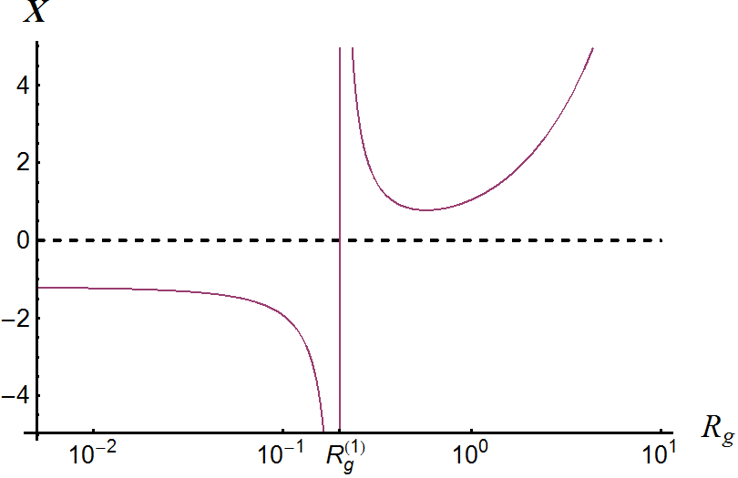
Figure 7: The relative wave-energy input to the TKE pool, $X=(1-f)\,\Pi/P$, as a function of the gradient Richardson number, $R_{g}$. Negative $X$ indicate withdrawal of energy from the wave-energy pool and are physically irrelevant.

7 Geophysically shielded systems

These systems have no external sources of internal-wave energy but they are in coexistence equilibrium of turbulence and saturated waves with significant eigen-wave feedback, $f\ll 1$. Here $\Pi=0$ and the steady-state TKE balance reads in our notation as follows:

$$P=B^{\prime}+\tilde{B}+\varepsilon\,+f\,\Psi\,=B^{\prime}+\tilde{\gamma}\,\varepsilon\,+f\,\Psi\,.$$ (84)

The vorticity balance is

$$\eta=\frac{\varepsilon}{P}=\frac{\Omega^{2}}{S^{2}}=\frac{1}{2}+(1-f)\,\frac{Y}{\tilde{\gamma}}\,,$$ (85)

where for young waves, $f\approx 1$, the effect of $Y$ is negligible and the situation is close to the wind-tunnel case. Not so for older wave spectra.

We combine (84) and (85) and get after some algebra the following steady-state condition,

$$2=4R_{g}\left(1-\frac{2\,\tilde{\gamma}\,R_{g}}{\tilde{\gamma}+2\,(1-f)\,Y}\right)+\tilde{\gamma}+2\,(1-f)\,Y\,,$$ (86)

where $Y$ appears as a function of the steady-state Richardson number $R_{g}^{s}$, and of the ‘wave age’ $1-f$. The solution $Y=Y(R_{g}^{s})$ of (88) is presented in Fig. 8 for $f=0$.

The above means that with $Y$ we have a tunable parameter which allows us to adjust our model value for $R_{g}^{s}$ according to measurements or observations. Unfortunately these are rare for shielded conditions described above so that we are inclined to choose according to tradition the value $R_{g}^{s}=1/4$, which corresponds to $Y=0.136$. Another choice would be the minimum value of $Y$ which is 0.135 and corresponds to $R_{g}^{s}=0.265$. This somewhat arbotrary situation probably explains the large scatter in the measurements of $\sigma$ and underlines umso mehr the necessity of dedicated experiments and observational programmes.

We note in closing this Section that the more general form of the steady-state vorticity balance is

$$\eta=\frac{\varepsilon}{P}=\frac{\Omega^{2}}{S^{2}}=\frac{1}{2}+\frac{X+(1-f)\,Y}{\tilde{\gamma}}\,,$$ (87)

where the external forces $X\propto\Pi/P$ appear together with the feedback via eigen waves, $Y$. Our values of $Y$ are situated well below the validity limit of $X$. In the geophysically shielded case ($X=0$) and young waves ($f\approx 1$) the action of $Y$ is screened and we have $\eta=1/2$, which is the wind tunnel situation. In the same case with adult spectra ($f\ll 1$) we have the classical shielded case.

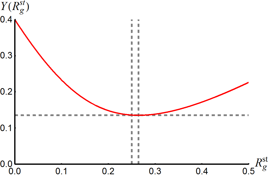
Figure 8: The parameter $Y$ as a function of the steady-state gradient Richardson number $R_{g}^{st}$ and for $f=0$. The horizontal and the right vertical dashed gray lines cross at the minimum of the function $Y$. The left vertical dashed line labels $R_{g}^{st}=\hbox{$\,{}^{1}\!/_{4}$}$. Values $Y\approx 0.135\dots 0.15$ would correspond to mathematically admissible values $R_{g}^{st}\approx 0.15\dots 0.3$.

8 Application

In the previous Sections of this report we have looked at special physical situations which we knew and understood sufficiently well. Now we put these pieces together and write down the full equation system for applications also to unknown situations. We choose here the philosophy of non-stationary embedding. At a first glance the associated evolution equations (88 – 99) look voluminous compared with the lean system of their purely algebraic steady-state counterparts, but non-stationary embedding avoids stiffness problems right on the most fundamental level and is thus substantially more robust in the computational practice.

8.1 Generalized equations

For an effective notation we define the following differential operator,

$${\cal D} = \left(\frac{\partial}{\partial t}-\frac{\partial}{\partial z}\,\nu\,\frac{\partial}{\partial z}\right),$$ (88)

$$\tilde{\cal D} = \left(\frac{\partial}{\partial t}-\frac{\partial}{\partial z}\,\tilde{\nu}\,\frac{\partial}{\partial z}\right),$$ (89)

so that the general set of balances can be written for a stratified water column as follows:

$${\cal D}\,\Omega = \frac{1}{\pi}\left[\frac{S^{2}}{2}+\frac{1-f}{1+\tilde{\Gamma}}\left(\frac{\Pi}{P}+Y\right)S^{2}-\Omega^{2}\right],$$ (90)

$$\tilde{\cal D}\,{\cal K} = \Pi+P-\nu\left[f\,\Psi+\frac{N^{2}}{\sigma}+(1+\tilde{\Gamma})\Omega^{2}\right]$$ (91)

$$\tilde{\cal D}\,{\cal E} = \Pi+\Psi-c_{1}\,{\cal E}-c_{2}\,{\cal E}^{2}\;,$$ (92)

$$f(t) = \frac{c_{1}\,{\cal E}}{c_{1}\,{\cal E}+c_{2}\,{\cal E}^{2}}\,,$$ (93)

$$\sigma = \frac{\sigma_{0}}{1-N^{2}/\Omega^{2}}\;,$$ (94)

$$P = \nu\,S^{2}\;,$$ (95)

$$\Psi = \frac{P}{\sigma_{0}}\,\frac{S^{2}}{\Omega^{2}}\;R_{g}^{2}\,,$$ (96)

$$\nu = {\cal K}/{\pi\,\Omega}\,,$$ (97)

$$\mu = {\nu}/\sigma\,,$$ (98)

$$R_{g} = N^{2}/S^{2}\,.$$ (99)

To apply this theory in form of a numerical model it needs to be combined with a scheme which provides us with the mean-flow variables from which we may derive the shear $S$ and the Brunt-Väisälä frequency, $N$. Furthermore we need initial conditions for all variables. But the hydrodynamic system is highly dissipative and ‘forgets’ the initial conditions soon such that here “reasonable guesses” would suffice.

8.2 The parameters

8.2.1 Overview.

$\tilde{\Gamma}=0.2$ and $\sigma_{0}=1/2$ are universal constants. $f$ is a function of time. Its final equilibrium value, $f_{\infty}$, depends on the molecular-viscosity parameter $c_{1}$. In many cases it is sufficient to set $f_{\infty}=0$.

With the exception of $\tilde{\nu}$, the whole system contains only one tunable paramter, $Y\sim{\cal O}(10^{-1})$. The inner physical structure of $Y$ (and $\tilde{\Gamma}$) we have not yet fully understood. I.e. we are not able to derive its value from other than pragmatic arguments like ‘it works’, because it gives the right gradient Richardson number for the geophysically shielded steady-state.

About the spatial ‘diffusivity’ of wave packets, $\tilde{\nu}$, we only know that it scales with the characteristic group velocity $\langle c_{g}\rangle$ of the wave packets, multiplied by a characteristic length scale which is possibly the characteristic wave lenght of a packet:

$$\tilde{\nu} \propto \langle c_{g}\rangle\times\cal L\,.$$ (100)

The last open problem to be discussed is the role of $\Pi$. According to Gregg (1989) it can be estimated from the r.m.s. 10-meter wave shear, $\langle S_{10}^{2}\rangle$, as function of time and of the region of the world ocean under study. This will be done in the next Subsection.

8.3 Wave-induced dissipation: the ocean case

The above results apply to stratified oceanic and atmospheric flows as well. The following estimator of the long-wave, non-local (“external”) energy source $\Pi$ is based on extensive studies in the world oceans and is thus not automtically applicable to atmospheric conditions. For the latter a comparable result is unknown.

Gregg (1989) presented a summary of comprehensive, extensive and direct dissipation and stadardized shear observations ($S_{10}$) made in ocean waters around the globe, where the following conditions applied at least approximately:

• There was almost no mean-flow shear, $S\approx 0$.

• The IGW field was almost perfectly saturated, $f\approx 0$.

• The observations were done for conditions of quasi-steady state, $d\Omega/dt=d{\cal K}/dt=d{\cal E}/dt=0$.

Gregg established the following empirical relation between the wave-induced dissipation rate, $\tilde{\varepsilon}$, the 10-meter high-pass filtered vertical shear, $S_{10}=\Delta U/10\,\mbox{m}$, and the effective Brunt-Väisälä frequency, $\langle N^{2}\rangle^{1/2}$:

$$\tilde{\varepsilon} = a_{1}\,\frac{\langle N^{2}\rangle}{N_{0}^{2}}\;\frac{\langle S_{10}^{4}\rangle}{S_{GM}^{4}}\;.$$ (101)

Very low frequencies have been removed from $S_{10}$ by filtering. The average in $\langle S_{10}^{4}\rangle$ is taken over longer observation periods.

$S_{GM}$ used in (101) is the so-called Garrett-Munk shear:

$$S_{GM}^{4} = a_{2}\,\frac{\langle N^{2}\rangle^{2}}{N_{0}^{4}},$$ (102)

with the following empirical parameters:

$$a_{1} = 7\times 10^{-10}\;\mbox{m${}^{2}$\,s${}^{-3}$}\,,$$ (103)

$$a_{2} = 1.66\times 10^{-10}\;\mbox{s${}^{-4}$}\,,$$ (104)

$$N_{0} = 5.2\times 10^{-3}\;\mbox{s${}^{-1}$}\,.$$ (105)

We insert (102) in (101) and get

$$\tilde{\varepsilon} = a_{3}\,\frac{\langle S_{10}^{4}\rangle}{\langle N^{2}\rangle}\,,$$ (106)

where

$$a_{3} = \frac{a_{1}}{a_{2}}\,N_{0}^{2}\;\;=\;\;1.14\times 10^{-4}\;\mbox{m}^{2}\,\mbox{s}^{-1}\,.$$ (107)

We further take into account that (see Gregg, 1989)

$$\langle S_{10}^{4}\rangle = 2\,\langle S_{10}^{2}\rangle^{2}$$ (108)

such that (106) may be written as follows,

$$\tilde{\varepsilon} = a_{4}\,\frac{\langle S_{10}^{2}\rangle^{2}}{\langle N^{2}\rangle}\;=\;a_{4}\,\frac{\langle S_{10}^{2}\rangle}{\tilde{R}_{g}}\,,$$ (109)

with the wave-based gradient Richardson number,

$$\tilde{R}_{g} = \frac{\langle S_{10}^{2}\rangle}{\langle N^{2}\rangle}.$$ (110)

The latter needs to be unterschieden von the mean-field based gradient Richardson number $R_{g}=\langle N^{2}\rangle/\langle S\rangle^{2}$. The parameter $a_{4}$ reads as follows:

$$a_{4} = 2\,a_{3}\;\;=\;\;2.3\times 10^{-4}\;\mbox{m${}^{2}$\,s${}^{-1}$}\,.$$ (111)

With (109) we have a solid estimate of $\Pi$ as

$$\Pi= = (1+\tilde{\Gamma})\,\varepsilon\;=\;\;a_{4}\,(1+\tilde{\Gamma})\,\frac{\langle S_{10}^{2}\rangle}{\tilde{R}_{g}}\,,$$ (112)

so that herewith the model system is completely closed and we can begin with simulations, provided we have a certain knowledge about the wave-field parameters $\langle S_{10}^{2}\rangle$ and $\tilde{R}_{g}$ for our ocean or atmosphere region of interest.

9 Comparison with observations

During the about 15-years walk towards the system (88 – 99) partial solutions were step by step confronted with corresponding observational and experimental data. The totality of these theory-observation comparisons cannot be repeated here. We refer for the wind-tunnel experiments to Baumert and Peters (2004, 2005), for the Monin-Obukhov boundary layer to Baumert (2005a), for the neutrally stratified case to Baumert (2005b, 2012). These specific cases are well described by subsets of (88 – 99), corresponding individually to the special physical situation studied.

With respect to a theory-data comparison the present article thus concentrates on the case $R_{g}\gg 1$ where without mentioning it $R_{g}$ means here always an equilibrium or steady-state value. We look namely on the relation $\sigma=\sigma(R_{g})$, analyzed and summarized by Zilitinkevich et al. (2008). These authors used more or less the same comprehensive data base for their discussions like Galperin et al. (2007), Canuto et al. (2008) and Kantha and Carniel (2009). In the core these are the CASES-99 (stable nocturnal BL, see Poulos et al., 2002) and the SHEBA experiments (arctic BL over ice; see Grachev et al., 2005, 2006).

Zilitinkevich et al. (2008) conclude that the class-wise average of the data is best described by $\sigma=0.8+5\,R_{g}$ shown in full red in Fig. 9. In our view this line is somewhat above the CASES-99 data and our alternative theoretically derived relation, $\sigma=(1+{5}\,R_{g})/2$, fits better. It is given in full green in Fig. 9 and located somewhat below the full-red curve. Of course, in view of the enormous scatter of the original data, the red and the green lines are well within the huge overall scatter range.

The two blue lines (full and dashed blue) in Fig. 9 represent our simulation results in good agreement with the observations of CASES-99. At the same time they might illustrate why natural data exhibit such a strong scatter. While the dashed blue line is the case $f=0.5\,\%$, the full blue line stands for $f=0$. I.e. very small absolute variations in $f$ cause large variations in the solutions. Generally the huge scatter might be caused by the varying age (or degree of saturation) of the waves involved. These waves are mostly of non-local origin so that in principle all points of the distant space are candidates for their birth places and any age of arriving waves can be expected at our study site. On the one hand structural equilibrium needs to be achieved to avoid such a scatter. This appears to be difficult under the action of waves which also modify the flow. But still more important seems to be the different age of the incoming wave spectra.

According to our theory Fig. 9 shows also the two new critical gradient Richardson numbers for the wave-turbulence coexistence in form of two vertical thin black dashed lines at $R_{g}^{(1)}=(1-\tilde{\Gamma})/4=0.2$ and $R_{g}^{(2)}=(1-\tilde{\Gamma})/2=0.4$. The higher value labels the lower applicability limit of our theory.

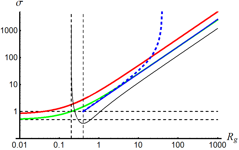
Figure 9: Turbulent Prandtl number as function of the gradient Richardson number for various coexistence equilibria of turbulence and internal waves. The theory in dashed blue contains the relative viscous energy loss of the wave field, $f$, taken here as $0.5\,\%$. Zilitinkevich et al. (2008) recommend as a phenomenological rule the relation $\sigma\approx 0.8+5\times\,R_{g}$ (full, red), which does not contain the pole visible in the CASES-99 data and our $f=0.5\;\%$ case. Only in the case $f=0$ our theory gives a straight line (full blue) which gives asymptotically $\sigma=(1+5\times R_{g})/2$ (full green). The thin black dashed vertical lines indicate the positions 0.2 and 0.4. The thin black horizontal lines label 0.5 and 1.

10 Discussion

This report may be seen as an experiment to draw a (dotted) theoretico-physical bottom line under more than 50 years of ambitious observational programs and experimental laboratory research into stratified small-scale geophysical and engineering turbulence and mixing processes. Looking backwards, today these programs appear as a single planned initiative wherein mutually supplementing pieces fit perfectly together. On the water side the efforts took place in the United States and the United Kingdom. On the atmospheric side also multi-national efforts need to be acknowledged. Our results may encourage those who believe that the “turbulence problem” (Hunt, 2011) is eventually solvable.