High zenith angle observations of PKS 2155-304 with the MAGIC-I telescope

Abstract

Context. The high frequency peaked BL Lac PKS 2155-304 with a redshift of z=0.116 was discovered in 1997 in the very high energy (VHE, E$>$100 GeV) $\gamma$-ray range by the University of Durham Mark VI $\gamma$-ray Cherenkov telescope in Australia with a flux corresponding to 20% of the Crab Nebula flux. It was later observed and detected with high significance by the Southern Cherenkov observatory H.E.S.S. establishing this source as the best studied Southern TeV blazar. Detection from the Northern hemisphere is difficult due to challenging observation conditions under large zenith angles. In July 2006, the H.E.S.S. collaboration reported an extraordinary outburst of VHE $\gamma$-emission. During the outburst, the VHE $\gamma$-ray emission was found to be variable on the time scales of minutes and with a mean flux of $\sim$7 times the flux observed from the Crab Nebula. Follow-up observations with the MAGIC-I standalone Cherenkov telescope were triggered by this extraordinary outburst and PKS 2155-304 was observed between 28 July to 2 August 2006 for 15 hours at large zenith angles.

Aims. We studied the behavior of the source after its extraordinary flare. Furthermore, we developed an analysis method in order to analyze these data taken under large zenith angles.

Methods. Here we present an enhanced analysis method for data taken at high zenith angles. We developed improved methods for event selection that led to a better background suppression.

Results. The quality of the results presented here is superior to the results presented previously for this data set: detection of the source on a higher significance level and a lower analysis threshold. The averaged energy spectrum we derived has a spectral index of ($-3.5\pm 0.2$) above 400 GeV, which is in good agreement with the spectral shape measured by H.E.S.S. during the major flare on MJD 53944. Furthermore, we present the spectral energy distribution modeling of PKS 2155-304. With our observations we increased the duty cycle of the source extending the light curve derived by H.E.S.S. after the outburst. Finally, we find night-by-night variability with a maximal amplitude of a factor three to four and an intranight variability in one of the nights (MJD 53945) with a similar amplitude.

1 Introduction

The blazar PKS 2155-304 is the so-called lighthouse of the Southern hemisphere. The high frequency peaked BL Lac PKS 2155-304, at a redshift of z=0.116, was discovered in the VHE $\gamma$-ray range by the University of Durham Mark VI $\gamma$-ray Cherenkov telescope (Australia) in 1997 with a flux corresponding to $\sim$0.2 times the Crab Nebula flux (Chadwick et al. 1999). PKS 2155-304 was confirmed as a TeV $\gamma$-ray source by the H.E.S.S. group after observations in 2002 and 2003 (Aharonian et al. 2005a). In July 2006, the H.E.S.S. collaboration reported an extraordinary outburst of VHE $\gamma$-emission (Aharonian et al. 2007). During this outburst, the $\gamma$-ray emission was found to be variable on time scales of minutes with a mean flux of $\sim$7 times the flux observed from the Crab Nebula for E$>$200 GeV. Large amplitude flux variability at these time scales implies that the TeV emission originates from a small region due to the requirement that light travel times must be sufficiently short in the frame of the emitting region. Follow-up observations of the outburst by the MAGIC telescope were triggered in a Target of Opportunity program by an alert from the H.E.S.S. collaboration (Benbow et al. 2006). The results of this campaign are presented in this paper. The CANGAROO group also observed the source immediately after the flare, obtaining a significance of 4.8 $\sigma$ and an averaged integral flux above 660 GeV that corresponds to $\sim$45% of the flux observed from the Crab Nebula (Sakamoto et al. 2008). The H.E.S.S. collaboration continued observations and detected 44 hours later again a major VHE flare. The data were taken contemporaneously with the Chandra satellite and a strong correlation between the X-ray and the VHE $\gamma$-ray bands was found (Aharonian et al. 2009a). MAGIC observed on six consecutive nights following the trigger and here we present the final results of the data set. Due to observational constraints, MAGIC did not observe the source during the major flares, but in two cases data were taken immediately afterwards, part of the data being simultaneous with H.E.S.S. and Chandra data. Two years later, in 2008 another multi-wavelength campaign was performed providing simultaneous MeV-TeV data taken by the Fermi Gamma-ray Space Telescope and the H.E.S.S. experiment (Aharonian et al. 2009b). With these data the low state of the source could be modeled, including high energy data for the first time. All these observations establish this source as the best studied Southern TeV blazar.

Blazars are Active Galactic Nuclei whose relativistic plasma jets nearly point towards the observer. The overall (radio to $\gamma$-ray) spectral energy distribution (SED) of these objects shows two broad non-thermal continuum peaks. For high energy peaked BL Lac objects (HBLs), the first peak of the SED covers the UV/X-ray bands whereas the second peak is in the multi GeV band. There are various models to explain this spectral shape. They are generally divided into two classes: leptonic and hadronic. Both models attribute the peak at keV energies to synchrotron radiation from relativistic electrons (and positrons) within the jet, but they differ on the origin of the TeV peak. The leptonic models advocate the inverse Compton scattering mechanism, utilizing synchrotron self Compton (SSC) interactions and/or inverse Compton interactions with an external photon field, to explain the VHE emission, (e.g. Maraschi et al. (1992); Dermer et al. (1992); Sikora et al. (1994)). On the other hand, hadronic models account for the VHE emission through initial p-p or p-gamma interactions or via proton synchrotron emission (e.g. Mannheim (1993); Aharonian (2000); Pohl & Schlickeiser (2000)).

Blazars often show violent flux variability, which may or may not be correlated between the different energy bands. Strictly simultaneous observations are crucial to investigate these correlations and understand the underlying physics of blazars.

The structure of the paper is the following: In section 2 we introduce the MAGIC telescope. In section 3 we present a new analysis method optimized for large zenith angle (ZA) observations. We test the method on Crab Nebula data taken under large zenith angles (60^∘ to 66^∘) in section 4.1. In section 4.2 we apply the method to the PKS 2155-304 data set and in addition, we model the spectrum in section 4.2.3. We summarize the results in section 5.

2 The MAGIC telescope

The MAGIC collaboration operates two 17 m diameter Imaging Cherenkov Telescopes on the Canary Island of La Palma. The data set presented here was taken in 2006, i.e. before the second MAGIC telescope was installed. Therefore, only single telescope data are available for this analysis. The camera of the MAGIC phase I telescope has hexagonal shape with a field of view (FoV) of $\approx$ 3.5^∘ mean diameter and comprises 576 high-sensitivity photomultiplier tubes. The energy resolution is $\Delta$E/E=20% above 200 GeV. The single telescope flux sensitivity for a point-like source is 1.6% of the Crab Nebula flux for a 5$\sigma$ detection in 50 hrs of on-source time. The energy threshold is about 50-60 GeV at the trigger level. Further details of telescope parameters and on the performance can be found in Baixeras et al. (2004); Cortina et al. (2005); Albert et al. (2008b). These performance values are valid for observations at small zenith angles, where the distance between the extended air shower and the telescope is the shortest.

In the case of PKS 2155-304 the observations had to be conducted at high ZA (up to 66^∘) since this source culminates at 58^∘ ZA in La Palma. Under these special conditions a larger effective area is achieved and sources from a large section of the Southern sky can be observed with a threshold of a few hundred GeV ($\approx$ 100 GeV-500 GeV, zenith angle dependent). Observations at such high ZA not only produce a significantly higher threshold, but also usually result in a considerable loss of sensitivity. The analysis presented here is a re-analysis of the data presented in Mazin & Lindfors (2008). The goal of this re-analysis was to improve the results, obtain a more significant detection and a lower analysis threshold.

3 Data Analysis

All data analyzed in this work were taken in wobble mode, i.e. tracking a sky direction, which is 0.4^∘ off the source position and alternating it every twenty minutes to the opposite side of the camera center. These changes avoid effects caused by camera inhomogeneities. The background is estimated from the mirrored source position in the same FoV, which improves the background estimation and yields a better time coverage because no extra OFF data have to be taken. In this analysis we use three OFF regions which are distributed at angles of 90^∘, 180^∘ and 270^∘ from the source position with respect to the camera center. These OFF regions have the same size and the same distance from the camera center.

The analysis presented here improves on the original one of Mazin & Lindfors (2008) in several aspects. It makes use of the pixel-wise timing information for the image cleaning, as well as in the background suppression, through the gradient of the signal arrival time along the major image axis. These improvements allow to reduce the energy threshold for these high zenith angle observations from $\sim$600 GeV to $\sim$300 GeV, and increase the overall significance of the excess from 11 to 25 standard deviations. In the following the analysis is explained in detail.

In this work we use the time image cleaning (Aliu et al. 2009): given the sub-nsec timing resolution of the data acquisition system and thanks to the parabolic structure of the telescope mirror a small integration window can be chosen. This reduces the number of pixels with signals due to night sky background which survive the image cleaning. A minimum number of 6 photoelectrons in the core pixels and 3 photoelectrons in the boundary pixels of the images are required. Differences between the signal arrival times have to be smaller than 1.75 ns. This allows a reduction in the pixel threshold level (i.e. retaining pixels with less charge) of the image cleaning, leading to a lower analysis energy threshold. The cleaned camera image is characterized by a set of image parameters based on Hillas (1985). These parameters provide a geometrical description of the images of the showers and are used to infer the energy of the primary particle, its arrival direction and to distinguish between $\gamma$-ray showers and hadronic showers.

Cosmic-ray background suppression is achieved by means of dynamical cuts in AREA versus SIZE (Riegel et al. 2005). Typically, events with low SIZE are rejected because the $\gamma$/ hadron separation is very poor for such images. A standard AREA cut for low zenith angle data is shown in Figure 1 by the blue line. This standard cut removes low SIZE events corresponding to events with low energies.

The angular distance, $\theta$, between the reconstructed direction of an event and the catalog position of the $\gamma$-ray source is an essential background rejection parameter. The event direction is obtained by using the DISP parameter (Lessard et al. 2001; Domingo-Santamaria et al. 2005), which uses the image shape to estimate where, along the major axis of the image, lies the point in the camera that corresponds to the shower direction. For a point-like $\gamma$-ray source, the distribution of $\theta^{2}$ will peak at around zero, whereas background events produce a rather flat distribution.

Analysis of data taken at high ZA requires special treatment compared to low ZA data. The Cherenkov light of the showers observed at large ZA has a longer optical path, as it has to pass a thicker layer of atmosphere. Therefore, the shower maximum is located farther from the observatory and the photon density of each shower decreases. This reduces the number of detectable showers, especially at low energies. The global effect is a shift of the energy threshold to higher energies with increasing ZA. At the same time, images taken at high ZA correspond, for a given value of SIZE, to events with higher amount of shower particles than at low ZA. The higher amount of shower particles reduces the intrinsic shower fluctuations. For this reason one obtains better defined $\gamma$-ray showers at high ZA. This implies that the minimum SIZE at which effective background suppression is possible can be lowered for high ZA compared to low ZA. In this section we quantify this effect.

A specialized parameterization of the AREA cut was developed for this high ZA study. Together with improving the cosmic-ray background rejection power, its main objective was to lower the energy threshold. A comparison between the standard AREA cut, which is used for the detection of the source, and the specialized parameterization, used for obtaining the spectrum, is shown in Figure 1. For a low energy analysis the parameterization of the spectrum cut is:

$$\textit{Area}<(1.4\cdot(\log_{10}(\textit{SIZE})-0.8)^{2}+1)\cdot x,$$ (1)

where x is varied between 0.007 and 0.009 to study the dependency of the spectrum from the cut efficiencies. The red points in Figure 1 represent Monte Carlo (MC) gammas and the black ones background events before cuts. The standard AREA cut used for the detection and the spectrum AREA cut are shown by the blue and the green parabolas, respectively. For the spectrum AREA cut, it can been seen that events with small SIZEs survive the background suppression.

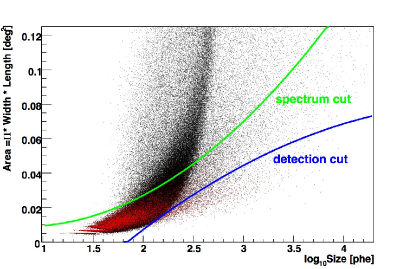
Figure 1: Red: Monte Carlo gammas at high ZA (60^∘-66^∘), black: Background events before cuts, blue: AREA cut used for the detection ($\theta^{2}$ plot) of the Crab Nebula, green: Specialized area parameterization used for the spectrum of the Crab Nebula.

A quantitative estimate for the background suppression power can be made with the quality factor Q:

$$Q=\frac{\epsilon_{\gamma}}{\sqrt{\epsilon_{bg}}},$$ (2)

where $\epsilon_{\gamma}$ is the fraction of $\gamma$-rays that are retained after a cut. $\epsilon_{bg}$ is the corresponding fraction of retained background events. To check that the background suppression with a combination of the new AREA cut and a $\theta^{2}$ cut is working for small SIZE-values, we calculate the Q-factor for the four lowest bins in SIZE (see table 1). For the AREA cut we require a $\gamma$-efficiency of 0.9 and for the $\theta^{2}$ cut one of 0.5. Having Q-factors (QHZA) in excess of 1 in each bin implies that the applied cut works efficiently. Comparing Q_HZA with the one obtained for low ZA (Q_LZA) shows a stronger background suppression power for the high ZA case. We also look closer into the rejection power of the AREA and $\theta^{2}$ cuts individually. First, we compare the hadron-efficiencies for the AREA cut at high ($\epsilon^{LZA}_{h}$) and low ZA ($\epsilon^{HZA}_{h}$). There is no difference between the two for $\log_{10}(\textit{SIZE})<2.0$ and there is a clear advantage for a high ZA analysis at higher SIZE values. Next we compare the $\theta^{2}$-distributions of MC $\gamma$-events for the lowest SIZE-bins at high and low ZA. We calculate the ratio of the $\theta^{2}$ cut values with 50% $\gamma$-ray event efficiency ($\theta^{2}_{LZA,50\%}$/$\theta^{2}_{HZA,50\%}$, see table 1). This fraction is directly proportional to the improvement of the background rejection at high ZA with respect to low ZA since the background has a flat distribution in the $\theta^{2}$-plot at $\theta^{2}<1$ deg². We obtain roughly 2 times better background suppression at high ZA than at small ZA for small SIZE values.

Table 1: Quality factors for high and low ZA analyses derived by using MC $\gamma$-events and real background events. Q-factor at high ZA: Q_HZA; Q-factor at low ZA: Q_LZA; hadron-efficiency of the AREA cut at low/ high ZA ($\gamma$-efficiency = 0.9): $\epsilon^{LZA}_{h}/\epsilon^{HZA}_{h}$, $\theta^{2}$-values at low/ high ZA ($\gamma$-efficiency = 0.5): $\theta^{2}_{LZA,50\%}$/$\theta^{2}_{HZA,50\%}$

SIZE-bin	QHZA	QHZA/QLZA	$\epsilon^{LZA}_{h}/\epsilon^{HZA}_{h}$	$\theta^{2}_{LZA,50\%}$/$\theta^{2}_{HZA,50\%}$
$\log_{10}(\textit{SIZE})$
1.5 – 1.75	1.06	1.25	1.0	1.92
1.75 – 2.0	1.51	1.45	1.0	2.30
2.0 – 2.25	2.27	1.49	1.13	2.58
2.25 – 2.5	4.44	1.73	2.0	2.0

In addition to the AREA cut, cuts are applied to timing parameters, which describe the time evolution along the major image axis and the RMS of the time spread. These two additional parameters lead to better background suppression, yielding a better sensitivity (Aliu et al. 2009).

A possible $\gamma$-ray signal coming from point-like sources can be identified with the directional information of the parameter $\theta$. The necessary signature of a $\gamma$-ray signal is an excess at small $\theta^{2}$ values, usually lower than 0.04 deg². The cuts used to calculate the significance of the detection and the cuts used to derive the energy spectrum of PKS 2155-304 were optimized on a Crab Nebula sample taken at large zenith angles (see 4.1 for details).

The primary $\gamma$-ray energies were reconstructed from the image parameters using a Random Forest regression method (Albert et al. 2008a) trained with MC simulated events (Heck & Knapp 2004; Majumdar et al. 2005). The MC sample is characterized by a power-law spectrum between 10 GeV and 30 TeV with a differential spectral photon index of $\alpha$=-2.6. The events were selected to cover the same ZA range as the data. Compared to the previous analysis (Mazin & Lindfors 2008) improvements are obtained because of an updated MC sample at high zenith angles leading to better agreement between data and MC.

Since the analysis technique described in this section is new, we first test its performance on a data set from a known, bright and stable $\gamma$-ray emitter: the Crab Nebula before applying the method to PKS 2155-304.

4 Results

4.1 Crab Nebula

The Crab Nebula is one of the best studied celestial objects because of the strong persistent emission of the Nebula over 21 decades of frequencies. It was the first object to be detected at TeV energies by the Whipple collaboration in 1989 (Weekes et al. 1989) and is the strongest steady source of VHE $\gamma$-rays. Due to the stability and the strength of the $\gamma$-ray emission the Crab Nebula is generally considered the standard candle of the TeV $\gamma$-ray astronomy. The measured $\gamma$-ray spectrum extends from 60 GeV (Albert et al. 2008b) up to 80 TeV (Aharonian et al. 2000) and appears to have maintained a constant flux in the VHE range over the years (from 1990 to present).

4.1.1 Data set and analysis sensitivity

In October 2007, the MAGIC telescope took Crab Nebula data with a zenith angle range of 60^∘ up to 66^∘. The data were taken under dark sky conditions and in wobble mode. After quality cuts an effective on-time of 2.15 hrs is obtained. Using detection cuts presented in section 3, Fig. 1 (i.e. optimized on significance of a separate Crab Nebula sample also taken at high zenith angles), a total of 247 excess events above 187 background events have been detected. The number of background events is obtained from three equally sized OFF regions and applying a geometrical scale factor of 0.33 (see Fig. 2). The significance of this $\gamma$-ray signal, obtained using Eq. 17 of Li & Ma (1983), is 12.8 $\sigma$. This corresponds to an analysis sensitivity of 8.7 $\frac{\sigma}{\sqrt{hour}}$. Using the same set of cuts we obtain the following sensitivities for integral fluxes ($\Phi$):

$$\Phi(E>0.4\,\mathrm{TeV}) \Rightarrow 5.7\%\mathrm{\,\,Crab\,\,in\,\,50\,hrs}$$

$$\Phi(E>0.63\,\mathrm{TeV}) \Rightarrow 5.6\%\mathrm{\,\,Crab\,\,in\,\,50\,hrs}$$

$$\Phi(E>1.0\,\mathrm{TeV}) \Rightarrow 5.9\%\mathrm{\,\,Crab\,\,in\,\,50\,hrs}$$

$$\Phi(E>1.5\,\mathrm{TeV}) \Rightarrow 6.8\%\mathrm{\,\,Crab\,\,in\,\,50\,hrs}$$

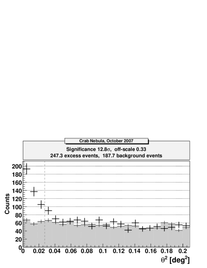
Figure 2: The ON-source and normalized background distribution of $\theta^{2}$. The ON-source is shown in the black crosses and the background is shown in the gray shaded region. 2.15 hrs of Crab data show an excess with a significance of 12.8$\sigma$.

4.1.2 Differential Energy Spectrum

Using the data set described in the previous section, we derived the differential energy spectrum of the Crab Nebula (see Fig. 3). The spectrum is well described by a simple power law of the form:

$$\frac{\mathrm{d}N}{\mathrm{d}E}=(2.7\pm 0.4)\cdot 10^{-7}\left(\frac{\mathrm{E}}{\mathrm{TeV}}\right)^{-2.46\pm 0.13}\left(\frac{\mathrm{ph}}{\mathrm{TeV}\,\mathrm{s}\,\mathrm{m}^{2}}\right).$$

The errors are statistical only. The gray band represents the range of results obtained by varying the total cut efficiency between 40% and 70%, i. e. the cut efficiency after applying the AREA and the $\theta^{2}$ cuts. For comparison, the Crab Nebula spectrum from data taken at low zenith angles is drawn as a dashed line (Albert et al. 2008b). A very good agreement has been found.

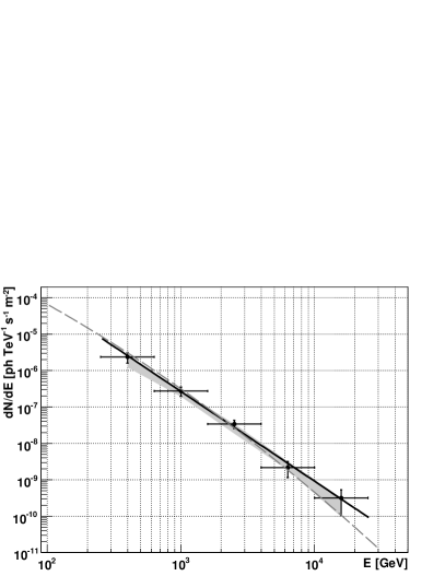
Figure 3: Differential energy spectrum of the Crab Nebula. Black line: power law fit to the data, gray band: systematic uncertainties of the analysis, dashed line: published data taken at low zenith angles (Albert et al. 2008b).

4.2 PKS 2155-304

The MAGIC telescope observed the blazar PKS 2155-304 from 28 July to 2 August 2006 (MJD 53944.09 – MJD 53949.22) over the zenith angle range of 59^∘ to 64^∘. The data were taken under dark sky conditions and in wobble mode. After quality cuts a total effective on-time of 8.7 hrs is obtained. For the detection of PKS 2155-304, the same cuts are used as for the detection of the Crab Nebula. Three OFF regions are used and 1029 excess events above 846 normalized background events are detected. A significance of 25.3 standard deviations is obtained, whereas with the previous analysis only 11$\sigma$ could be achieved . The corresponding $\theta^{2}$-plot is presented in Fig. 4.

Figure 4: The ON-source and normalized background distribution of $\theta^{2}$. The denotations are the same as in Figure 2. A clear excess with a significance of more than 25 standard deviations for a source at the position of PKS 2155-304 is found.

4.2.1 Differential Energy Spectrum

The differential energy spectrum for the whole data set is shown in Fig. 5 as a black line together with the spectrum of H.E.S.S. (dashed line), measured during the strong outburst (Aharonian et al. 2007). Note that H.E.S.S. and MAGIC data are not simultaneous. The spectral points obtained in this analysis are fitted in the energy range from 400 GeV to 4 TeV, because at lower energies H.E.S.S. reported a change of the slope ($-3.53\pm 0.05$ above 400 GeV to $-2.7\pm 0.06$ below 400 GeV). The fitted MAGIC data points are consistent with a power law:

$$\frac{\mathrm{d}N}{\mathrm{d}E}=(1.8\pm 0.2)\cdot 10^{-7}\left(\frac{\mathrm{E}}{\mathrm{TeV}}\right)^{-3.5\pm 0.2}\left(\frac{\mathrm{ph}}{\mathrm{TeV}\,\mathrm{s}\,\mathrm{m}^{2}}\right)$$

with a fit probability after the $\chi^{2}$-test of 81%. Above 400 GeV, the energy flux measured by H.E.S.S. from the preceding flare of PKS 2155-304 is one order of magnitude higher than the flux measured by MAGIC. It is interesting to note that although the flux measured with H.E.S.S. is higher, the spectral slope remains the same within the statistical errors.

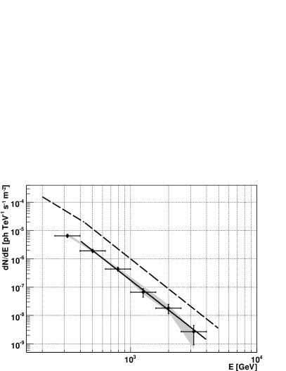
Figure 5: Differential energy spectrum (black line) for the whole data set together with systematic errors obtained by varying cuts efficiencies (gray band). The black dashed line corresponds to the H.E.S.S. measurement during the flare.

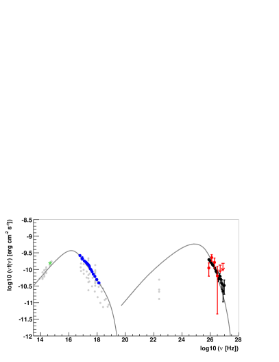
Figure 6: The overall spectral energy distribution (SED) of PKS 2155-304 from optical wavelengths through VHE $\gamma$-rays. The gray line denotes an SSC model as in Krawczynski et al. (2004). The effect of the EBL is taken into account by using the model of Franceschini et al. (2008). Red points: MAGIC, red arrows: MAGIC 2 $\sigma$ upper limits, black: H.E.S.S., blue: Chandra, green star: optical point (ROTSE). All data were taken simultaneously on the day MJD 53946 with exception of the ROTSE point and they are taken from Aharonian et al. (2009a). Selected historical data from infrared to $\gamma$-rays are shown in gray for comparison reasons (Giommi et al. 2002).

4.2.2 Account of EBL attenuation in $\gamma$-ray spectra

For the VHE-spectra in Fig. 6, representing data from the day MJD 53946, the absorption effect caused by the extragalactic background light (EBL) was taken into account. The VHE photons interact with the low-energy photons of the EBL (Gould & Schréder 1966; Hauser & Dwek 2001). The predominant reaction $\gamma_{VHE}+\gamma_{EBL}\rightarrow e^{+}e^{-}$ leads to an attenuation of the intrinsic AGN spectrum $\mathrm{d}N/\mathrm{d}E_{intr}$ that can be described by

$$\mathrm{d}N/\mathrm{d}E_{obs}=\mathrm{d}N/\mathrm{d}E_{intr}\cdot\exp[-\tau_{\gamma\gamma}(E,z)]$$

with the observed spectrum $\mathrm{d}N/\mathrm{d}E_{obs}$, and the energy dependent optical depth $\tau_{\gamma\gamma}(E,z)$. We apply the EBL model of Franceschini et al. (2008) which is the same as the H.E.S.S. collaboration used to account for EBL attenuation in their spectrum, and which agrees well with other state-of-the-art EBL models (Kneiske & Dole 2010; Domínguez et al. 2011; Gilmore et al. 2011).

4.2.3 Spectral energy distribution and SSC modeling

SSC models have been very successful in describing the observed HBL multi-frequency spectra. In the homogeneous one-zone SSC model, the X-ray emission comes from synchrotron radiation emitted by a population of high energy electrons, followed by inverse Compton scattering of synchrotron photons to TeV energies, which explains the $\gamma$-ray emission from TeV blazars. Based on this model it is possible to constrain the parameter space of the emission region and estimate its basic parameters, the Doppler factor, $D$, and the rest-frame magnetic field, $B$, of the emitting plasma in the relativistic jet.

The acceleration region is approximated by a spherical ”blob” with radius $R$ and bulk Lorentz factor $\Gamma$ that is moving along the jet under a small angle $\theta$ to the line of sight. The blob contains relativistic electrons of density $\rho$ accelerated by shock acceleration processes. It is assumed that the energy spectrum of the electrons in the jet frame can be described by a broken power law with low-energy ($E_{min}$ to $E_{break}$) and high-energy ($E_{break}$ to $E_{max}$) indices $n_{1}$ and $n_{2}$, respectively ($n_{i}$ is from $\mathrm{d}N/\mathrm{d}E\propto E^{-n_{i}}$; E is the electron energy in the jet frame). The electron spectrum has exponential cut-offs at energies $E_{min}$ and $E_{max}$.

For a successful modeling simultaneous multi-wavelength information is required. In Fig. 6 almost simultaneous data taken on 30 July 2006 with MAGIC, H.E.S.S. and Chandra are shown. The data taken by Chandra are contemporaneous with those taken with MAGIC. Please note that we scaled the spectrum obtained by H.E.S.S., since the data are not entirely contemporaneous with the MAGIC data. The data for the spectrum computed by H.E.S.S. are from MJD 53946.013–53946.129, whereas the MAGIC data are obtained slightly later between MJD 53946.092–53946.186. These time spans are represented in Fig. 9. This difference is large enough to produce a difference in the average fluxes by almost a factor of 3. We scaled the H.E.S.S. spectrum down by this factor and get a good agreement with the MAGIC result. For the modeling we did not take into account the optical data point from ROTSE, because this measurement was taken before the high state of the source.

We modeled the multi-wavelength spectrum (Fig. 6, gray line) with a one-zone, time independent SSC code from Krawczynski et al. (2004). This ”by-eye” adjustment of model parameters, instead of e.g. $\chi^{2}$-minimization, is a common procedure with data of this kind because of degeneracy of the model and rather large uncertainty in the data. In Fig. 9 we show in colored bars the time span of data we used for the SED modeling. Note that the data set we modeled was taken few hours after the flare and no significant variability is seen in H.E.S.S. or MAGIC data (see Fig. 9), which justifies usage of a time independent model. Still, the time independent model should be taken with caution. The resulting model parameters shown in Table 2 provide a possible solution in the SSC model parameter space. The parameters are similar to the ones typically obtained for HBLs, see e.g. Aharonian et al. (2005b); Aleksić et al. (2012): the Doppler factor is high and the magnetic field strength is low. It has been pointed out that such high Doppler factors are in conflict with what is seen on VLBA (Piner et al. 2010), but this issue is beyond the scope of this paper.

Table 2: Parameters for SED modeling

Doppler factor	$B$	$R$	$\rho$	$E_{min}$	$E_{max}$	$E_{break}$	$n1$	$n2$
	[T]	$[\mathrm{m}]$	$[\mathrm{particle/cm^{3}}]$	$\lg(E_{min}[\mathrm{eV}])$	$\lg(E_{max}[\mathrm{eV}])$	$\lg(E_{break}[\mathrm{eV}])$
50	$0.085\times 10^{-4}$	$0.9\times 10^{14}$	0.07	6.3	11.5	10.2	2	4

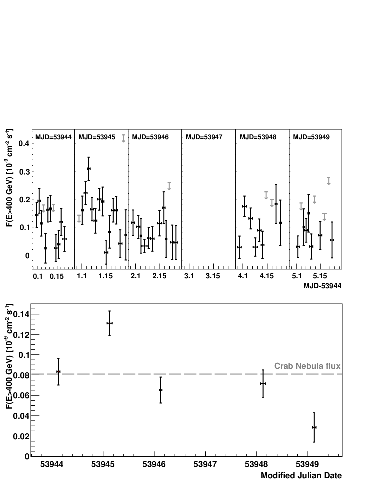
Figure 7: Top: MAGIC light curve for individual nights for E$>$400 GeV of PKS 2155-304. Only the second night (MJD 53945) shows significant intra-night variability. Vertical arrows represent flux upper limits at a confidence level of 95%. Bottom: Light curve for the total data set for E$>$400 GeV with one flux point per night. The error bars in x-direction represent the observation time. The Crab Nebula flux is shown for comparison. For more information see the text.

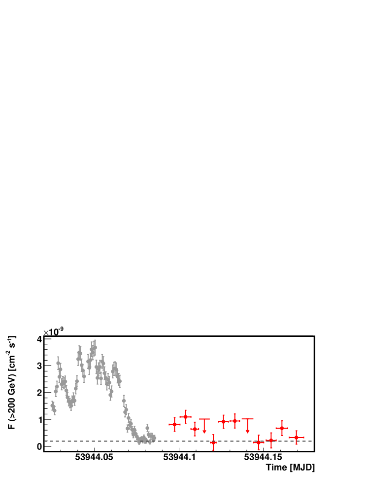
Figure 8: Integral flux above 200 GeV of the first flare observed from PKS 2155-304 on MJD 53944 versus time measured by H.E.S.S. (gray points) and by MAGIC (red points). The MAGIC points are obtained using the integral flux above 400 GeV and extrapolated down to 200 GeV using the derived photon spectral index of -3.5. Instead, assuming the spectral index of -2.7 below 400 GeV as found by H.E.S.S., the MAGIC points would be 24% lower in flux. The horizontal line represents the observed flux of the Crab Nebula (Aharonian et al. 2006).

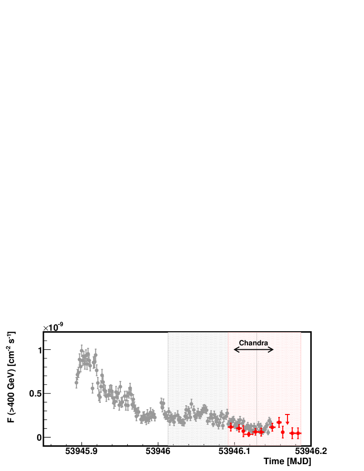
Figure 9: Light curve of PKS 2155-304 of the second flare observed by MAGIC and H.E.S.S. in the night of July 29-30, 2006. The flux is shown above an energy of 400 GeV. The MAGIC data (red points) are binned in 10 minute intervals while the H.E.S.S. data (gray points) use four minute intervals. The red and the gray area represent the time spans when the MAGIC and the H.E.S.S. spectra shown in Fig. 6 are derived, respectively. The black arrow shows the time when Chandra observed the source.

4.2.4 Light curves

Figure 7 shows the integral light curves for energies above 400 GeV. In the upper panel, each point corresponds to an average flux every two data runs (roughly 10 min exposure), whereas in the lower panel each point corresponds to an average flux per night. Significant detections in most of the time bins are obtained. A significant intra-night variability is found for the second night MJD 53945 (29 July 2006) giving a probability for a constant flux of less than $5\times 10^{-9}$. For the other nights, no significant intra-night variability is found. In the lower panel of Fig. 7, a night-by-night light curve is shown. A fit by a constant to the run-by-run light curve results in a chance probability of less than $10^{-12}$. However, a fit by a constant to the night-by-night light curve results in a chance probability of $1\times 10^{-6}$. We, therefore, conclude that there is a significant variability on the time scales reaching from days (largest scale we probed) down to 20 minutes (shortest scale we probed).

In Fig. 8 we show the MAGIC light curve with data taken directly after the first major flare detected by H.E.S.S. (28 July 2006) (Aharonian et al. 2007). The MAGIC points are binned in 10 minute intervals and the H.E.S.S. points have a binning of one minute intervals (Aharonian et al. 2009a). After the large flare, with a measured flux above 200 GeV of up to 15 times the flux of the Crab Nebula (Aharonian et al. 2007), the source returned to a lower state, with fluxes of the order of 1 Crab. The second flare observed by H.E.S.S. is shown in Fig. 9. MAGIC observed the source in the low state simultaneous with H.E.S.S. on 30 July 2006. The measurements are in good agreement concerning the trend of the data points, but the MAGIC data points appear to lie systematically below the points obtained by H.E.S.S. The observed difference in the flux is compatible with the systematic uncertainty of the analysis, which has been estimated to be 20% of the energy scale or 50% on the flux level. Typically, the systematic energy scale uncertainty for analysis of Imaging Cherenkov telescope data is at the level of 15% to 20%, see e.g. (Meyer et al. 2010). The difference we find in this analysis is at the upper edge of the usual systematic uncertainty, which may be due to additional systematics of measurements at high zenith angles where details of the atmosphere are less certain.

5 Conclusions

A study of the high-zenith angle performance of the MAGIC telescope (operating in single-telescope mode) was carried out with observations of the source PKS 2155-304 during a high state, conducted between ZA 60^∘ - 66^∘. A new analysis procedure was used in this work in order to enhance the sensitivity of the observations under these special conditions, for instance, included information about the signal arrival times to improve the image cleaning and background subtraction.

We tested this new analysis method on a Crab data sample and obtained a sensitivity of 5.7% of the Crab Nebula flux for 50 hrs of observations at high ZA above 0.4 TeV. The differential energy spectrum of the Crab Nebula is in excellent agreement with the published data at lower zenith angles. This improved analysis is used to reanalyze data of PKS 2155-304 taken with MAGIC in 2006.

The energy spectrum of the whole data set from 400 GeV up to 4 TeV has a spectral index of ($-3.5\pm 0.2$). As it agrees with the index derived by the H.E.S.S. collaboration during the flaring state of the source, we conclude that the spectrum does not show any change in its spectral slope with flux state above 400 GeV. Furthermore, we corrected the measured spectrum for the effect of the EBL absorption using the model of Franceschini et al. (2008) and made an SED modeling of simultaneous data in the VHE and X-ray energy range.

The light curves derived with MAGIC show a significant variability on daily as well as on intra-night time scales. The MAGIC observations immediately after the extraordinary flare measured by H.E.S.S. on MJD 53944 indicate that the source remained essentially constant for the rest of that night. The measurements of the MAGIC and the H.E.S.S. experiments are generally in good agreement.

Finally, we conclude that high zenith angle observations with the MAGIC telescope have proven to yield high quality spectra and light curves above 300 GeV. With these observations we could extend the duty cycle of PKS 2155-304 observations, which is clearly convenient for the study of any flaring source. High-zenith angle observations, although challenging, generally allow for more uninterrupted coverage of highly variable sources. Also, future high ZA observations of some objects allow unique spectral measurements at higher energies than is possible at lower ZA by virtue of the larger effective area.