Generic flow profiles induced by a beating cilium

Abstract

We describe a multipole expansion for the low Reynolds number fluid flows generated by a localized source embedded in a plane with a no-slip boundary condition. It contains 3 independent terms that fall quadratically with the distance and 6 terms that fall with the third power. Within this framework we discuss the flows induced by a beating cilium described in different ways: a small particle circling on an elliptical trajectory, a thin rod and a general ciliary beating pattern. We identify the flow modes present based on the symmetry properties of the ciliary beat.

I Introduction

Cilia are thin cellular protrusions that beat in an asymmetric periodic fashion in order to propel the surrounding fluid Gray1928 ; Brennen.Winet1977 ; Sleigh74 . They are involved in swimming and feeding of a number of protozoa and also have many crucial functions in vertebrates. These include the mucous clearance in respiratory pathways, transport of an egg cell in Fallopian tubes, left-right symmetry breaking in embryonic development afzelius99 ; Hirokawa.Takeda2006 ; Supatto.Vermot2008 , and, recently discovered, otolith formation in hearing organs Colantonio.Hill2009 . Cilia have inspired designs for microfluidic pumps and mixers using similar beating patterns Vilfan.Babic2010 ; Kokot.Babic2011 ; Gauger.Stark2009 ; Toonder.Anderson2008 ; Coq.Bartolo2011 ; Hussong.Westerweel2011 ; Shields.Superfine2010 .

The beating pattern of a single cilium can be very complex and generally consists of a working stroke during which the stretched cilium moves the fluid in the direction of pumping and a recovery stroke during which the cilium folds and returns to the origin by sweeping along the surface, thereby minimizing the drag as well as backward flow. Especially when working in large ensembles, the beating patterns found in nature are remarkably close to the theoretically calculated optimum Osterman.Vilfan2011 . Despite this complexity, the flows can be described with a small number of generic terms in the far field, i.e., when we observe the flow at a distance $r$ which is sufficiently larger than the cilium length $L$. In the leading order the flow velocity falls as ${\cal O}(r^{-2})$ vilfan2006a .

In this paper we go beyond the quadratic order and provide a complete set of functions that describe the flow in the presence of a no-slip boundary. We then specifically discuss the ${\cal O}(r^{-3})$ terms that are present with different beating patterns, depending on their symmetry properties.

II Multipole expansion

II.1 In unbounded fluid

In the low Reynolds number regime, the motion of an incompressible fluid is described by the Stokes equation and the incompressibility condition:

$$\eta\Delta\mathbf{v} =\mathbf{\nabla}p$$ (1)

$$\mathbf{\nabla}\cdot\mathbf{v} =0\;.$$ (2)

To derive the general form of the flow induced by a localized distribution of forces and/or sources we follow the approach of Lamb Lamb , also used by Happel and Brenner Happel.Brenner . Note that this is just one of many complete sets of far-field solutions (see Ref. Pozrikidis1992 for a derivation in Cartesian coordinates). Although the basis set we will derive can be obtained more directly as spatial derivatives of known solutions (Stokeslet and source), the following construction has several advantages. First, we know from the beginning on that we are dealing with a complete set of linearly independent solutions. Second, these solutions will appear classified by their angular symmetry, which are useful for the description of flows induced by cilia which also share some of these symmetries. And finally, the construction allows us to distinguish between different solutions (e.g., with or without a pressure gradient).

Multiplying Eq. (1) with $\mathbf{\nabla}\cdot$ immediately leads to a Laplace equation for the pressure

$$\Delta p=0\;.$$ (3)

The solution of the homogeneous equation in the absence of pressure gradients ($\Delta\mathbf{v}=0$) can be written as $\mathbf{v}=\mathbf{\nabla}\times(\mathbf{r}\chi)+\mathbf{\nabla}\Phi$, where $\chi$ and $\Phi$ are two solutions of the Laplace equation. In total we need three sets of harmonic functions ($p$, $\chi$ and $\Phi$) to construct the general solution of the Stokes equation in unbounded space. We now introduce a spherical coordinate system such that

$$\mathbf{x}=\left(\begin{array}[]{c}r\sin\theta\cos\phi\\ r\sin\theta\sin\phi\\ r\cos\theta\end{array}\right)\;.$$ (4)

If there is no external flow, i.e, the $\lim_{r\to\infty}\mathbf{v}(\mathbf{x})=0$, the multipole expansion of the velocity field reads

$$\mathbf{v}=\sum_{l=0}^{\infty}\mathbf{v}_{l}\qquad\text{with}\;\mathbf{v}_{l}\sim r^{-(l+1)}$$ (5)

with

$$\mathbf{v}_{l}=\nabla\times(\mathbf{r}\chi_{l})+\nabla\Phi_{l-1}\\ +\frac{1-l}{2\eta(1+l)(1+2l)}r^{2}\nabla p_{l+1}+\frac{2+l}{\eta(1+l)(1+2l)}\mathbf{r}p_{l+1}$$ (6)

and

$$\chi_{l} =\frac{1}{r^{l+1}}\sum_{m=-l}^{l}A_{lm}e^{im\phi}P_{l}^{m}(\cos\theta)$$ (7)

$$\Phi_{l-1} =\frac{1}{r^{l}}\sum_{m=-(l-1)}^{(l-1)}B_{lm}e^{im\phi}P_{l-1}^{m}(\cos\theta)$$ (8)

$$p_{l+1} =\eta(1+l)(1+2l)\frac{1}{r^{l+2}}\sum_{m=-(l+1)}^{(l+1)}C_{lm}e^{im\phi}P_{l+1}^{m}(\cos\theta)\;.$$ (9)

The coefficients $A_{lm}$ are defined for $l\geq 1$ and $|m|\leq l$, $B_{lm}$ are defined for $l\geq 1$ and $|m|\leq l-1$ and $C_{lm}$ for $l\geq 0$ and $|m|\leq l+1$. Using an elementary vector identity the first term in (6) can alternatively be written as $(\mathbf{\nabla}\chi_{l})\times\mathbf{r}$. Inserting these terms into Eq. (6) gives the expression for the velocity

$$\mathbf{v}_{lm}=\frac{e^{im\phi}}{r^{l+1}}\Bigl{[}\Bigl{(}A_{lm}P_{l}^{\prime m}(\cos\theta)\sin\theta+B_{lm}\frac{im}{\cos\theta}P_{l-1}^{m}(\cos\theta)\\ +C_{lm}\frac{1-l}{2}\frac{im}{\sin\theta}P_{l+1}^{m}(\cos\theta)\Bigr{)}\hat{e}_{\phi}\\ +\Bigl{(}A_{lm}\frac{im}{\sin\theta}P_{l}^{m}(\cos\theta)-B_{lm}P_{l-1}^{\prime m}(\cos\theta)\sin\theta\\ -C_{lm}\frac{1-l}{2}P_{l+1}^{\prime m}(\cos\theta)\sin\theta\Bigr{)}\hat{e}_{\theta}\\ +\Bigl{(}-B_{lm}lP_{l-1}^{m}(\cos\theta)+C_{lm}\frac{(l+1)(l+2)}{2}P_{l+1}^{m}(\cos\theta)\Bigr{)}\hat{e}_{r}\Bigr{]}$$ (10)

In the unbounded space, the leading terms have the order $l=0$ and represent the 3 components of a Stokeslet. Their magnitude is given by the coefficients $C_{0,-1}$, $C_{0,0}$ and $C_{0,1}$. In the next order, $l=1$, representing terms that decay as $1/r^{2}$, we have 3 solutions for the $\chi$ component, 1 for $\Phi$ and 5 for $p$, 9 in total. In general, the number of terms of order $l$ is

$$N_{l}=3+6l\;.$$ (11)

Note that all these solutions can be constructed from derivatives of 4 fundamental solutions. These include 3 Stokeslets ($l=0,m=0,\pm 1$) and a source $l=1,m=0$. We denote these solutions as ${\cal G}_{x}$, ${\cal G}_{y}$, ${\cal G}_{z}$ and $\cal S$. The remaining solutions can be constructed from derivatives like $\partial_{x}{\cal G}_{x}$, $\partial_{y}{\cal G}_{x}$ etc.

II.2 Bounded by a no-slip plane

As the cilium (or any other source of fluid pumping) is embedded in a plane, we have to find the solutions that fulfill the boundary condition

$$\mathbf{v}(r,\theta=\pi/2,\phi)=0\;.$$ (12)

We first note that this condition has to be satisfied for all $r$ and $\phi$ values, which means that we can collect terms with the same indices $l$ and $m$ and then form all independent linear combinations that fulfill the boundary condition.

When expressing $\mathbf{v}_{lm}$ in the plane (at $\theta=\pi/2$) we have to distinguish between even and odd values of $l+m$. If $l+m$ is even, so is the associated Legendre polynomial $P_{l}^{m}(x)$, implying $\left.\frac{d}{dx}P_{l}^{m}(x)\right|_{x=0}=0$. For an odd $l+m$, $P_{l}^{m}(x)$ is an odd function so that $P_{l}^{m}(0)=0$. Of course, we have to take into account that the terms with an even $l+m$ actually contain $\Phi$ and $p$ terms with an odd $l+m$, because they contain spherical harmonics of the order $l-1$ and $l+1$, respectively. In total the condition that $\mathbf{v}_{lm}(r,\pi/2,\phi)=0$ for an even $l+m$ implies

$$imA_{lm}P_{l}^{m}(0)-B_{lm}P_{l-1}^{\prime m}(0)-\frac{1-l}{2}C_{lm}P_{l+1}^{\prime m}(0)=0$$ (13)

This condition is generally fulfilled by 2 independent solutions. For example, we can choose the coefficients $A_{lm}$ and $C_{lm}$ freely, but then have to determine $B_{lm}$ from (13). However, when $m=\pm l$, there is a single solution, because there is no $\Phi$ ($B$) term. When $l=m=0$ there is neither a $\Phi$ nor a $\chi$ term, so there is no solution of this order.

For an odd $l+m$ the boundary condition leads to two equations

$$A_{lm}P_{l}^{\prime m}(0)+imB_{lm}P_{l-1}^{m}(0)+im\frac{1-l}{2}C_{lm}P_{l+1}^{m} =0$$

$$-lB_{lm}P_{l-1}^{m}(0)+\frac{l^{2}+3l+2}{2}C_{lm}P_{l+1}^{m}(0) =0$$ (14)

These equations generally have a single solution for each pair $l$, $m$.

Table 1: Number of linearly independent solutions for each pair of numbers $l$ and $m$.

$m$	0	$\pm 1$	$\pm 2$	$\pm 3$	$\pm 4$ …	Total
$l=0$	0					0
1	1	1				3
2	2	1	1			6
3	1	2	1	1		9
4	2	1	2	1	1	12
$\vdots$						$\vdots$
$l$						$3l$

It is now time to count the total number of independent solutions for each $l$. An overview is given in Table 1. For any $l\geq 1$, we have

$$N_{l}=3l$$ (15)

solutions, down from $3+6l$ in the unbounded space.

In the following we will have a closer look at the terms that decay quadratically with the distance ($l=1$) and those that decay with the third power ($l=2$).

II.3 $l=1$: Modes of the order $r^{-2}$

In this order we have $N_{1}=3$ modes: one of them ($m=0$) represents a fluid source and two ($m=\pm 1$) the flow of two horizontal Stokeslets in the proximity of the boundary.

The source is described by the second and the fourth term in Eq. (6) alone. The solution for the pressure is $p_{10}\propto\frac{1}{r^{3}}\frac{3\cos^{2}\theta-1}{2}$, that for the second term $\Phi_{00}\propto 1/r$. The resulting velocity is

$$S(\mathbf{x})=\frac{1}{r^{2}}\cos^{2}\theta\hat{e}_{r}=\frac{z^{2}}{r^{5}}\left(\begin{array}[]{c}x\\ y\\ z\end{array}\right)\;.$$ (16)

To distinguish it from a source in bulk we call this term “surface sourcelet”. Note that because of volume conservation beating cilia naturally do not act as a source. But the source is one of the fundamental singularities and we will later show that its derivatives can be used to express higher order terms that are present. Also, this formalism could be used in a more general context – the source could describe fluid injection through a pore in the surface, or, temporarily, the flow around an expanding bubble.

The solutions with $m=\pm 1$ represent two horizontal Stokeslets. In this order there is no $\Phi$ term and the $\chi$ term has to vanish ($A_{lm}=0$) in order to fulfill the boundary condition (13). The velocities are determined by the last term in Eq. (6) and stem from pressure terms $p_{2,\pm 1}\propto\frac{1}{r^{3}}e^{\pm im\phi}\cos\theta\sin\theta$. We can construct the first from $\mathbf{v}_{1,1}+\mathbf{v}_{1,-1}$

$$D_{x}=\frac{1}{r^{2}}\cos\theta\sin\theta\cos\phi\hat{e}_{r}=\frac{xz}{r^{5}}\left(\begin{array}[]{c}x\\ y\\ z\end{array}\right)$$ (17)

and the second from $\mathbf{v}_{1,1}-\mathbf{v}_{1,-1}$

$$D_{y}=\frac{1}{r^{2}}\cos\theta\sin\theta\sin\phi\hat{e}_{r}=\frac{yz}{r^{5}}\left(\begin{array}[]{c}x\\ y\\ z\end{array}\right)\;.$$ (18)

We will call these terms “surface Stokeslets”. With 3 linearly independent solutions we know that we have a complete set for the order $v\propto r^{-2}$.

The surface sourcelet $S$ and the two surface Stokeslets $D_{x}$ and $D_{y}$ are shown in Figure 1.

$S$

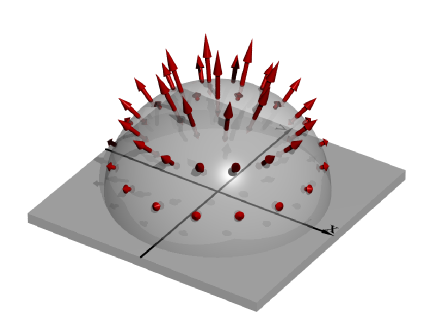
$D_{x}$

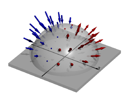
$D_{y}$

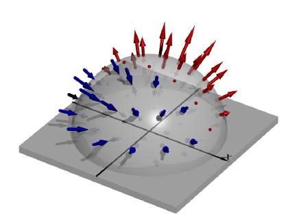
Figure 1: Fundamental modes of the order $r^{-2}$. For each mode the angular dependence of the velocity field is shown along a semi-transparent hemisphere. The colour of the arrows denotes inbound and outbound flow. The three depicted modes are a “surface sourcelet” $S$ and two “surface Stokeslets” $D_{x}$ and $D_{y}$.

Note that these 3 modes represent a fundamental set. All higher order terms can be constructed by deriving them by $x$ and $y$. We can see this from the fact that we have counted $3l$ solutions of order $l$. To get from the fundamental solutions to those of order $l$ we have to derive them $l-1$ times by the coordinates, which gives us $l$ linearly independent derivatives (unlike in unbounded fluid they all are independent). So we have shown that in total $3l$ derivatives of the fundamental solutions represent a complete set of solutions to that order. We will nevertheless derive the solutions from the spherical harmonics directly in order to collect modes according to their angular symmetry - this system is very convenient to discuss the ciliary flows.

II.4 $l=2$: Modes of the order $r^{-3}$

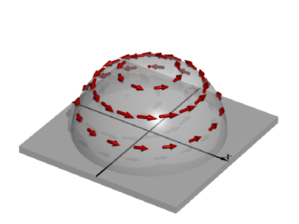
$Q_{1}$ $Q_{2}$

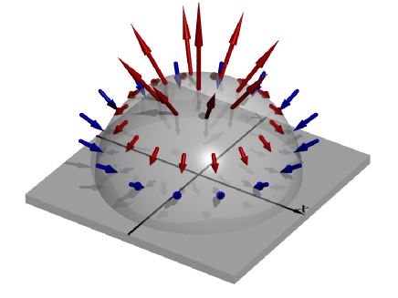
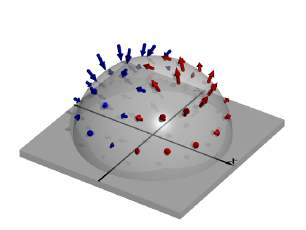
$Q_{3}$ $Q_{4}$

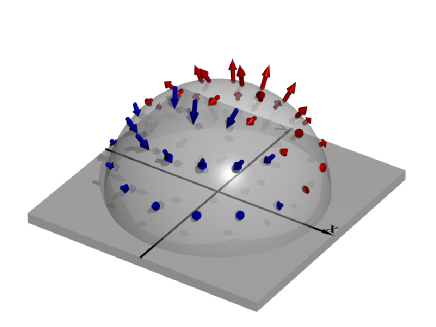
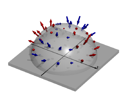
$Q_{5}$ $Q_{6}$

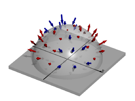
Figure 2: Six modes of the order $r^{-3}$: The surface rotlet $Q_{1}$, the vertical Stokeslet $Q_{2}$, the surface source doublets $Q_{3}$ and $Q_{4}$ and surface stresslets $Q_{5}$ and $Q_{6}$.

In this order we have a total of 6 independent terms, two with $m=0$, two with $m=\pm 1$ and two with $m=\pm 2$.

The first solution can be obtained from $\chi_{2,0}\propto\frac{1}{r^{3}}\frac{3\cos^{2}\theta-1}{2}$:

$$Q_{1}=\frac{1}{r^{3}}\sin\theta\cos\theta\hat{e}_{\phi}=\frac{z}{r^{5}}\left(\begin{array}[]{c}-y\\ x\\ 0\end{array}\right)\;.$$ (19)

This is a rotlet around the $z$ axis.

The second solution is obtained from $\Phi_{1,0}$ and $p_{3,0}$. It reads

$$Q_{2} =\frac{1}{r^{3}}\left((4\cos^{3}\theta-2\cos\theta)\hat{e}_{r}+\cos^{2}\theta\sin\theta\hat{e}_{\theta}\right)$$

$$=\frac{z}{r^{7}}\left(\begin{array}[]{c}(5z^{2}-2r^{2})x\\ (5z^{2}-2r^{2})y\\ (5z^{2}-3r^{2})z\end{array}\right)\;$$ (23)

and corresponds to the flow of a vertical Stokeslet near the boundary plane Blake.Chwang1974 . The fluid is moved outwards along the $z$ axis and inwards along the $x-y$ plane. Note that this is the only axisymmetric term – it is therefore clear that this is the leading term describing acoustic streaming caused by ultrasonic oscillations of a small bubble on a planar surface Marmottant.Hilgenfeldt2006 .

The modes with $m\pm 1$ that fulfill the boundary condition (II.2) are

$$Q_{3} =\Re\frac{1}{r^{3}}\left(4\cos^{2}\theta\sin\theta\hat{e}_{r}-\cos^{3}\theta\hat{e}_{\theta}-i\cos^{2}\theta\hat{e}_{\phi}\right)e^{i\phi}$$

$$=\frac{z^{2}}{r^{7}}\left(\begin{array}[]{c}5x^{2}-r^{2}\\ 5xy\\ 5xz\end{array}\right)$$ (27)

$$Q_{4} =\Im\frac{1}{r^{3}}\left(4\cos^{2}\theta\sin\theta\hat{e}_{r}-\cos^{3}\theta\hat{e}_{\theta}-i\cos^{2}\theta\hat{e}_{\phi}\right)e^{i\phi}$$

$$=\frac{z^{2}}{r^{7}}\left(\begin{array}[]{c}5xy\\ 5y^{2}-r^{2}\\ 5yz\end{array}\right)$$ (31)

They represent the fields of a horizontal rotlet (around the $y$ and $x$ axes) in the presence of a boundary. As we will see later, they can also be viewed as source-sink pairs (source-doublets) on the surface.

Finally, the modes with $m=\pm 2$, which have to fulfill the boundary condition (13) are

$$Q_{5} =\Re\frac{1}{r^{3}}\sin\theta\cos\theta\left(4\sin\theta\hat{e}_{r}-\cos\theta\hat{e}_{\theta}-i\hat{e}_{\phi}\right)e^{2i\phi}$$

$$=\frac{z}{r^{7}}\left(\begin{array}[]{c}(5(x^{2}-y^{2})-r^{2})x\\ (5(x^{2}-y^{2})+r^{2})y\\ 5(x^{2}-y^{2})z\\ \end{array}\right)$$ (35)

$$Q_{6} =\Im\frac{1}{r^{3}}\sin\theta\cos\theta\left(4\sin\theta\hat{e}_{r}-\cos\theta\hat{e}_{\theta}-i\hat{e}_{\phi}\right)e^{2i\phi}$$

$$=\frac{z}{r^{7}}\left(\begin{array}[]{c}(10x^{2}-r^{2})y\\ (10y^{2}-r^{2})x\\ 10xyz\\ \end{array}\right)$$ (39)

These modes represent surface stresslets. $Q_{5}$ is generated if a pair of forces pulls the fluid apart along the $x$ axis and another pair together along the $y$ axis. $Q_{6}$ is similar, but rotated by $45^{\circ}$ about the $z$ axis.

Like in unbounded space Pozrikidis1992 all these modes can be represented by derivatives of the $\sim r^{-2}$ modes in the following way:

$$Q_{1} =\frac{\partial D_{x}}{\partial y}-\frac{\partial D_{y}}{\partial x}$$ (40)

$$Q_{2} =\frac{\partial D_{x}}{\partial x}+\frac{\partial D_{y}}{\partial y}$$ (41)

$$Q_{3} =-\frac{\partial S}{\partial x}$$ (42)

$$Q_{4} =-\frac{\partial S}{\partial y}$$ (43)

$$Q_{5} =-\frac{\partial D_{x}}{\partial x}+\frac{\partial D_{y}}{\partial y}$$ (44)

$$Q_{6} =-\frac{\partial D_{x}}{\partial y}-\frac{\partial D_{y}}{\partial x}$$ (45)

These relations indicate that the modes $Q_{1}$, $Q_{2}$, $Q_{5}$ and $Q_{6}$ can be seen each as the flow of four point forces at an infinitesimal distance, as well as infinitesimally close to the surface. $Q_{3}$ and $Q_{4}$ represent a dipole consisting of a source and a sink. This representation is illustrated in Fig. 3.

Figure 3: Six modes of the order $r^{-3}$ represented with fundamental $r^{-2}$ solutions.

II.5 Higher order modes

In each higher order $l$, we have $N_{l}=3l$ modes that fall off with the power $r^{-(l+1)}$. All of them can be constructed from the derivatives

$$\frac{\partial^{l-1}S}{\partial x^{j}\partial y^{l-1-j}}\;,\qquad\frac{\partial^{l-1}D_{x}}{\partial x^{j}\partial y^{l-1-j}}\;,\;\text{and}\qquad\frac{\partial^{l-1}D_{y}}{\partial x^{j}\partial y^{l-1-j}}\;.$$ (46)

Unlike in unbounded fluid all these derivatives are linearly independent.

II.6 Normal form of the flow profile

Ciliary flows are characterized by the fact that they do not contain a source, but they do generate directional flow, so at least one of the terms $D_{x}$ and $D_{y}$ is present. By rotating the coordinate system, we can always bring the time-averaged flow to the form $\bar{\mathbf{v}}(\mathbf{x})={\cal A}D_{x}+{\cal O}(r^{-3})$.

To next order, the flow now has the shape

$$\bar{\mathbf{v}}(\mathbf{x})={\cal A}D_{x}(\mathbf{x})+\sum_{i=1}^{6}{{\cal B}_{i}}D_{i}(\mathbf{x})+{\cal O}(r^{-4})\;.$$ (47)

If we transform the coordinate system to $\mathbf{x^{\prime}}=\mathbf{x}-d_{x}\hat{e}_{x}-d_{y}\hat{e}_{y}$, we have

$$\bar{\mathbf{v}}^{\prime}(\mathbf{x}^{\prime})=\bar{\mathbf{v}}(\mathbf{x}^{\prime}-d_{x}\hat{e}_{x}-d_{y}\hat{e}_{y})\\ ={\cal A}\left(D_{x}(\mathbf{x^{\prime}})-d_{x}\frac{\partial D_{x}}{\partial x}(\mathbf{x^{\prime}})-d_{y}\frac{\partial D_{x}}{\partial y}(\mathbf{x^{\prime}})\right)\\ +\sum_{i=1}^{6}{{\cal B}_{i}}D_{i}(\mathbf{x}^{\prime})+{\cal O}(r^{-4})\;.$$ (48)

As we know from Eqns. (40-45) the derivatives are

$$\frac{\partial D_{x}}{\partial x} =\frac{Q_{2}-Q_{5}}{2} \frac{\partial D_{x}}{\partial y} =\frac{Q_{1}-Q_{6}}{2}$$ (49)

and by choosing $d_{x}=-\frac{2{\cal B}_{5}}{\cal A}$ and $d_{y}=-\frac{2{\cal B}_{6}}{\cal A}$ we can eliminate the modes $Q_{5}$ and $Q_{6}$. Of course, this transformation is only possible if ${\cal A}\neq 0$. Thus we have brought the stationary flow to the normal form

$$\bar{\mathbf{v}}^{\prime}(\mathbf{x}^{\prime})={\cal A}D_{x}(\mathbf{x^{\prime}})+\sum_{i=1}^{4}{{\cal B}^{\prime}_{i}}D_{i}(\mathbf{x}^{\prime})+{\cal O}(r^{-4})\;.$$ (50)

To summarize, with the proper choice of the coordinate system the static flow generated by a cilium can be described up to the order $r^{-3}$ with only 5 components: the surface Stokeslet $D_{x}$, the surface rotlet $Q_{1}$, the vertical surface Stokeslet $Q_{2}$, and the surface source-doublets $Q_{3}$ and $Q_{4}$. Because we can only transform the coordinate system once, for the static flow, we cannot reduce the oscillatory flows in the same way.

Figure 4: a) The volume flow rate $Q$ is defined as the fluid flux through a half-plane perpendicular to the surface and to the direction of pumping. b) Above a densely ciliated surface the flow becomes homogeneous with the average velocity $v_{c}$.

II.7 Volume flow rate

The performance of a cilium is characterized by the volume flow rate $Q$, defined as the average flux through a half-plane perpendicular to the direction of pumping Smith.Gaffney2008 , Fig. 4a. For example, for the mode corresponding to the pumping in $x$-direction with amplitude $\cal A$, $\mathbf{v}(x,y,z)={\cal A}D_{x}(x,y,z)$ has the volume flow rate

$$Q=\int_{-\infty}^{\infty}dy\int_{0}^{\infty}dz\,v_{x}(x,y,z)=\frac{2}{3}{\cal A}\;.$$ (51)

Due to volume conservation the flow rate is, of course, independent of the $x$-position of the cross-section chosen. Similarly, the volume flow rate of the mode $D_{y}$ would be defined as the flux through a half-plane with a constant $y$.

For the source, the flow rate is the actual influx. For a flow with $\mathbf{v}(x,y,z)={\cal A}S(x,y,z)$, the flow rate is

$$Q=\frac{2\pi}{3}{\cal A}\;.$$ (52)

The volume flow rate for higher order modes ($l\geq 2$) is always zero - the easiest way to see this is from the fact that they can be represented as spatial derivatives of the fundamental modes.

II.8 Velocity above ciliated layer

Instead of a single cilium, we often deal with a densely ciliated surface (Fig. 4b). Let $\rho$ denote the surface density of those cilia. Then the velocity above an infinite array is

$$v_{c}=\int_{-\infty}^{\infty}dX\int_{-\infty}^{\infty}dY\rho{\cal A}D_{x}(x-X,y-Y,z)=\frac{2\pi}{3}\rho{\cal A}=\pi\rho Q\;,$$ (53)

which is independent of $z$. The second relationship expresses the velocity above a ciliated layer with the volume generated by each cilium. In this regime, one can simplify the description of cilia by replacing them with a surface slip term with velocity $v_{c}$ Julicher.Prost2009 .

III Ciliary models

The ciliary beating pattern is quite complex, but there are several simplified models that have the correct symmetry properties and capture the far-field flow patterns. The simplest of all is a model that replaces the cilium with a single small particle (radius $a$), moving periodically on a closed path, and was used in several models for ciliary synchronization vilfan2006a ; Uchida.Golestanian2010 ; Golestanian.Uchida2011 ; Uchida.Golestanian2011 ; Kotar.Cicuta2010 .

III.1 Cilium as a small sphere

We start our discussion by expanding the flow field of a small particle subject to force $\mathbf{F}$ in terms of $D$- and $Q$-modes. An exact solution for the flow has been derived by Blake Blake.1971 and is now sometimes referred to as Blake’s tensor:

$$\mathbf{v}_{\alpha}(\mathbf{x})=\sum_{\beta}\bigl{[}G_{\alpha\beta}^{S}(\mathbf{x}-\mathbf{R})-G_{\alpha\beta}^{S}(\mathbf{x}-\mathbf{\bar{R}})+2Z^{2}G_{\alpha\beta}^{D}(\mathbf{x}-\mathbf{\bar{R}})\\ -2ZG_{\alpha\beta}^{SD}(\mathbf{x}-\mathbf{\bar{R}})\bigr{]}F^{\beta}$$ (54)

where $\mathbf{R}=(X,Y,Z)$ is the position of the particle, $Z$ is its height above the plane, $\mathbf{\bar{R}}=(X,Y,-Z)$ is the position of its mirror image and

$$G_{\alpha\beta}^{S}(\mathbf{x}) =\frac{1}{8\pi\eta}\left(\frac{\delta_{\alpha\beta}}{\left|\mathbf{x}\right|}+\frac{{x}_{\alpha}{x}_{\beta}}{\left|\mathbf{x}\right|^{3}}\right)\;,$$ (55)

$$G_{\alpha\beta}^{D}(\mathbf{x}) =\frac{1}{8\pi\eta}(1-2\delta_{\beta z})\frac{\partial}{\partial x_{\beta}}\left(\frac{x_{\alpha}}{\left|\mathbf{x}\right|^{3}}\right)$$ (56)

and

$$G_{\alpha\beta}^{SD}(\mathbf{x}) =(1-2\delta_{\beta z})\frac{\partial}{\partial x_{\beta}}G_{\alpha z}^{S}(\mathbf{x})$$ (57)

are the fields of a Stokeslet, source doublet and a Stokeslet-doublet, respectively. A Taylor expansion of Blake’s expression for small particle located at $(0,0,Z)$ up to the order $Z^{2}$ reads

$$\mathbf{v}(\mathbf{x})=\frac{1}{8\pi\eta}\bigl{(}12Z\bigl{(}F_{x}D_{x}(\mathbf{x})+F_{y}D_{y}(\mathbf{x})\bigr{)}\\ +6Z^{2}\bigl{(}-F_{x}Q_{3}(\mathbf{x})-F_{y}Q_{4}(\mathbf{x})+F_{z}Q_{2}(\mathbf{x})\bigr{)}\bigr{)}\;.$$ (58)

As noted by Blake and Chwang Blake.Chwang1974 the horizontal forces $F_{x}$ and $F_{y}$ generate terms of the order $r^{-2}$, while the vertical force $F_{z}$ only generates terms $\sim r^{-3}$. If the particle is not located exactly on the $z$ axis, but in any point $(X,Y,Z)$, we can use the derivatives (40–45) to obtain an expression that is again exact up to the order $r^{-3}$:

$$\mathbf{v}(\mathbf{x}) =\frac{1}{8\pi\eta}\bigl{(}12Z\bigl{(}F_{x}D_{x}(\mathbf{x})+F_{y}D_{y}(\mathbf{x})\bigr{)}$$

$$+6Z^{2}\bigl{(}-F_{x}Q_{3}(\mathbf{x})-F_{y}Q_{4}(\mathbf{x})+F_{z}Q_{2}(\mathbf{x})\bigr{)}$$

$$+6ZXF_{x}(Q_{5}(\mathbf{x})-Q_{2}(\mathbf{x}))$$

$$+6ZYF_{x}(Q_{6}(\mathbf{x})-Q_{1}(\mathbf{x}))$$

$$+6ZXF_{y}(Q_{6}(\mathbf{x})+Q_{1}(\mathbf{x}))$$

$$+6ZYF_{y}(-Q_{5}(\mathbf{x})-Q_{2}(\mathbf{x}))\bigr{)}\;.$$ (59)

This equation provides a basis for discussing all models that replace the cilium with a point particle.

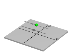
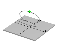
a)	b)	c)
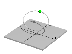
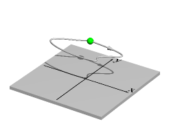
d)	e)	f)

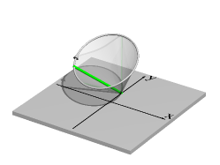
Figure 5: Models describing the ciliary beat as the motion of a small sphere along a closed trajectory: a) Linear, back-and-forth movement, which does not generate a directed flow. b) Planar elliptical trajectory. c) Tilted elliptical trajectory. d) General trajectory shape. e) General shape at a constant height. f) A model describing the cilium as a stiff slender rod.

III.1.1 Oscillating particle

We will start our discussion with a small particle, whose position is oscillating periodically parallel to the $x$-axis (Fig. 5a). Of course, this reciprocal motion will not generate any net (time-averaged) flow Purcell1977 . However, this type of motion has been studied as a model system for ciliary synchronization Kotar.Cicuta2010 ; Wollin.Stark2011 and therefore its far-field is of interest. It should also be noted that even if a single cilium performs reciprocal motion, an array of cilia with metachronal coordination can still generate directed flow Lauga2011 ; Khaderi.Onck2012 .

Since the motion is symmetric with respect to the $x-z$ plane, the only solutions that are theoretically possible are $D_{x}$, $Q_{2}$, $Q_{3}$ and $Q_{5}$.

We parameterize the particle motion as

$$\mathbf{R}(t)=\left(\begin{array}[]{c}B\sin\omega t\\ 0\\ D\end{array}\right)$$ (60)

so that the force acting on it is $\mathbf{F}=6\pi\eta aB\cos(\omega t)\hat{e}_{x}$. The resulting velocity field is

$$\mathbf{v}(\mathbf{x},t)=\frac{3\omega aBD}{4}\bigl{[}\sin(\omega t)\ (12D_{x}(\mathbf{x})-6DQ_{3}(\mathbf{x}))\\ -\sin(2\omega t)3B(Q_{2}(\mathbf{x})-Q_{5}(\mathbf{x}))\bigr{]}\;.$$ (61)

III.1.2 Planar beat

The next level of model is a planar ciliary beat. We model it with a small particle moving along an elliptical trajectory in the $x-z$ plane (Fig. 5b). Individually, planar cilia are rather inefficient Downton.Stark2009 , but nearly planar beating patterns can be found in respiratory epithelia, as well as in some microorganisms, such as Opalina Brennen.Winet1977 . Several models for ciliary synchronization study planar beating patterns Gueron.Blum1997 ; Guirao.Joanny2007 ; Lenz.Ryskin2006 . Because of the symmetry with respect to the $x-z$ plane, the solution will still consist of the following terms alone: $D_{x}$, $Q_{2}$, $Q_{3}$ and $Q_{5}$. The particle trajectory is now parameterized as

$$\mathbf{R}(t)=\left(\begin{array}[]{c}B\sin\omega t\\ 0\\ C\cos\omega t+D\end{array}\right)$$ (62)

and the force on the particle is $\mathbf{F}=6\pi\eta a(B\cos(\omega t)\hat{e}_{x}-C\sin(\omega t)\hat{e}^{z}$.

Based on the symmetry of the trajectory, which is invariant when we transform $x\to-x$ and $t\to-t$ simultaneously, we conclude that all terms that are even in $t$ have to be even in $x$. That reduces the possible terms to $D_{x}$ and $Q_{3}$. Conversely, the terms that are odd in time have to be odd in $x$, which restricts them to $Q_{2}$ and $Q_{5}$. The velocity field up to the frequency $\omega$ (we omit higher harmonics, which exist up to the frequency $3\omega$) reads

$$\mathbf{v}(\mathbf{x},t)=\frac{3\omega a}{4}\bigl{[}6BCD_{x}(\mathbf{x})-6BCDQ_{3}(\mathbf{x})\\ +(12BDD_{x}(\mathbf{x})-6BD^{2}Q_{3}(\mathbf{x}))\cos(\omega t)\\ +\frac{3}{8}B^{2}C(Q_{5}(\mathbf{x})-Q_{2}(\mathbf{x}))\sin(\omega t)\bigr{]}\;.$$ (63)

III.1.3 Tilted ellipse

More properties of a ciliary beat are captured by a model that describes it as a sphere, circling on a tilted elliptical trajectory vilfan2006a , as shown in Fig. 5c. It is described as

$$\mathbf{R}(t)=\left(\begin{array}[]{c}B\sin\omega t\\ A\cos\omega t\\ C\cos\omega t+D\end{array}\right)\;.$$ (64)

The ($x\to-x$, $t\to-t$) symmetry is still present, so that the stationary current can only consist of components $D_{x}$, $Q_{1}$, $Q_{3}$ and $Q_{6}$. It is

$$\mathbf{\bar{v}}(\mathbf{x})=\frac{3\omega a}{4}\bigl{[}6BCD_{x}(\mathbf{x})-6BCDQ_{3}(\mathbf{x})-6ABDQ_{1}(\mathbf{x})\bigr{]}\;.$$ (65)

The major difference between the tilted ellipse and the vertical ellipse is that the tilted one contains a $Q_{1}$ component, or a surface rotlet, as an obvious consequence of the rotation around the $z$ axis. In the case of a flat ellipse ($C=0$), this is the only stationary component.

III.1.4 General trajectory

Let us finally discuss the stationary velocity field of a small particle moving along an arbitrary periodic trajectory (Fig. 5d). According to Eq. (III.1) the velocity is

$$\mathbf{\bar{v}}(\mathbf{x})=\frac{9a}{T}\Bigl{[}D_{x}(\mathbf{x})\oint ZdX+D_{y}(\mathbf{x})\oint ZdY\\ -\frac{1}{2}Q_{3}(\mathbf{x})\oint Z^{2}dX-\frac{1}{2}Q_{4}(\mathbf{x})\oint Z^{2}dY\\ +\frac{Q_{5}(\mathbf{x})-Q_{2}(\mathbf{x})}{2}\oint ZXdX+\frac{Q_{6}(\mathbf{x})-Q_{1}(\mathbf{x})}{2}\oint ZYdX\\ +\frac{Q_{6}(\mathbf{x})+Q_{1}(\mathbf{x})}{2}\oint ZXdY-\frac{Q_{5}(\mathbf{x})+Q_{2}(\mathbf{x})}{2}\oint ZYdY\Bigr{]}$$ (66)

where $T$ denotes the period. The first two terms (through a coordinate rotation they can be reduced to just $D_{x}$) generally dominate and they show that the volume flow rate is proportional to the projection of the trajectory onto the vertical plane in the direction of pumping. An interesting special case arises when the particle does not move vertically, $Z={\rm const}$ (Fig. 5e). Then all integrals except those with $YdX$ and $XdY$ represent integration of a total differential along a closed path and therefore vanish. Equation (66) simplifies to

$$\mathbf{\bar{v}}(\mathbf{x})=\frac{9aZS}{T}Q_{1}(\mathbf{x})$$ (67)

where $S$ is the area of the trajectory, $S=\oint XdY=-\oint YdX$. Regardless of the exact shape of the trajectory, a particle moving in the horizontal plane only produces a surface rotlet in the order $r^{-3}$.

III.2 Stiff slender rod

The next level of complexity is to describe the cilium as a thin stiff rod. Although the hydrodynamic description in this model is more accurate than replacing the cilium with a small particle, the motion is even more restricted. At any time it is determined by two angles. There are different ways to calculate the forces on the cilium. The simplest is the local drag or resistive force theory (RFT) which assumes two constant friction coefficients for motion parallel and perpendicular to the orientation of the rod Lauga.Powers2009 . It has the advantage that it allows analytical calculation of the force distribution, while still giving good results. Alternatively, one could use the slender body theory (SBT), which includes hydrodynamic interactions for distances longer than a chosen cut-off Johnson.Brokaw1979 . Even better accuracy can be achieved by describing the cilium as a chain of spheres Gauger.Stark2009 ; Osterman.Vilfan2011 , a chain of regularized Stokeslets Ainley.Cortez2008 or with surface boundary elements Smith.2009 .

Within the resistive force theory the local drag is described by a tangential drag coefficient $C_{T}$ and a normal coefficient $C_{N}$ – in the case of a rod that is anchored with one end only the latter is relevant. From the force density, we can calculate the far-field fluid flow using Blake’s tensor (54) or its far field approximation (III.1).

A simple version of the slender rod model is obtained if the rod moves along the mantle of a tilted cone, as proposed by Smith and coworkers Smith.Gaffney2008 . The motion of a point on the cilium is then described as (Fig. 5f)

$$\mathbf{R}=s\left(\begin{array}[]{ccc}\sin\psi\sin\omega t\\ \cos\theta\sin\psi\cos\omega t-\sin\theta\cos\psi\\ \sin\theta\sin\psi\cos\omega t+\cos\theta\cos\psi\end{array}\right)+\frac{3L}{4}\left(\begin{array}[]{ccc}0\\ \sin\theta\cos\psi\\ 0\end{array}\right)\;.$$ (68)

with $s$ denoting the position parameter running from $0$ to $L$. We have placed the cone such that its center of weight, not the tip, lies on the $z$ axis. We will soon see that this way we eliminated the terms $Q_{5}$ and $Q_{6}$ and brought the flows to the normal form discussed in Section II.6. In RFT the force density on the cilium is simply the transverse drag coefficient, multiplied by the local velocity

$$\mathbf{f}=C_{N}\,\omega s\left(\begin{array}[]{ccc}\sin\psi\cos\omega t\\ -\cos\theta\sin\psi\sin\omega t\\ -\sin\theta\sin\psi\sin\omega t\end{array}\right)\;.$$ (69)

We obtain the far-field flow by inserting the force densities (69) and positions (68) into Eq. (III.1) and integrating over the length. The resulting average flow is

$$\mathbf{\bar{v}}(\mathbf{x})=\frac{C_{N}L^{3}\omega}{4\pi\eta}\sin^{2}\psi\Bigl{(}\sin\theta D_{x}-\frac{3}{4}L\cos^{2}\theta\cos\psi Q_{1}\\ -\frac{3}{4}L\sin\theta\cos\theta\cos\psi Q_{3}\Bigr{)}\;.$$ (70)

The first term is the well known surface Stokeslet term $D_{x}$, with an amplitude proportional to $\sin\theta\sin^{2}\psi$ Smith.Gaffney2008 , or the projection of the tip trajectory onto the $x-z$ plane. It is maximal for $\psi=\arctan\sqrt{2}$ and $\theta=\pi/2-\psi$. The second term, $Q_{1}$, is a surface rotlet and is maximal for $\theta=0$ (no tilt) and $\psi=\arctan\sqrt{2}$. The third term, $Q_{3}$, a surface source-doublet, appears almost inevitably along with the $D_{x}$ term.

An approximate value of the friction coefficient $C_{N}$ was given by Gueron and Liron Gueron.Liron1992

$$C_{N}=\frac{8\pi\eta}{1+2\ln(2q/a)}$$ (71)

where $a$ is the radius of the rod and $q$ some characteristic length scale of the order $\sqrt{La}$. A comparison with the Rotne-Prager approximation gives a more precise estimate of $C_{N}=1.22\pi\eta$ for the ratio $L/a=20$ Vilfan.Babic2012 .

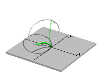
a)	b)
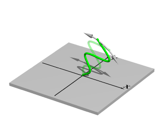
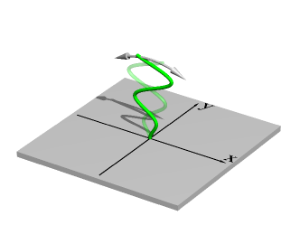
c)	d)

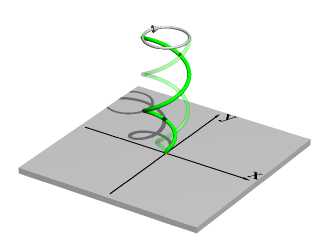
Figure 6: Beating patterns according to their symmetry properties. In each figure the faint line shows the cilium half a period later. a) A pattern symmetric upon mirroring in $x$ direction and simultaneous time reversal. b) A planar beating pattern. c) A planar pattern that is symmetric with respect to $x\to-x$, $t\to t+T/2$. d) A pattern symmetric with respect to rotation around $z$ axis and simultaneous time shift. This corresponds to a cilium rotating around the $z$ axis.

III.3 General

In the following we will discuss the flows generated by an arbitrary periodic beating pattern, based on its symmetry properties. Formally the problem could be solved numerically within the resistive force theory Blake1974 , as described in the previous section, although the motion would no longer be purely transversal, so the tangential friction coefficient would need to be included, too. Of course, any of the more accurate methods mentioned in the previous section can be applied.

A common symmetry of the beating pattern includes mirroring in the $x$ direction and simultaneous time reversal ($x\to-x$, $t\to-t$), Fig. 6a. The patterns discussed in Sections III.1.2, III.1.3 and III.2 all contain this symmetry. But note that many ciliary strokes found in nature do not. The typical recovery stroke during which the cilium bends and sweeps along the surface is not symmetric. Interestingly, the theoretically optimal solutions sometimes break this symmetry spontaneously and sometimes not, depending on the allowed radius of curvature Osterman.Vilfan2011 .

The symmetry property of the cilium trajectory has to be reflected in the stationary flow component

$$\mathbf{\bar{v}}(\mathsf{T}\mathbf{x})=s\mathsf{T}\mathbf{\bar{v}}(\mathbf{x})$$ (72)

with $s=-1$ and

$$\mathsf{T}=\left(\begin{array}[]{ccc}-1&0&0\\ 0&1&0\\ 0&0&1\end{array}\right)\;.$$ (73)

This condition is fulfilled by the modes $D_{x}$, $Q_{1}$, $Q_{3}$ and $Q_{6}$. Note that this holds for the time-averaged flow (stationary component). The oscillatory flow components can contain other modes.

Another interesting symmetric case is the general planar beating pattern (Fig. 6b). Then Eq. (72) holds with $s=1$ and

$$\mathsf{T}=\left(\begin{array}[]{ccc}1&0&0\\ 0&-1&0\\ 0&0&1\end{array}\right)\;.$$ (74)

It is fulfilled by modes $D_{x}$, $Q_{2}$, $Q_{3}$ and $Q_{5}$. An example of a planar beating pattern is a cilium producing a waving pattern, similar to a planar flagellum attached with one end to the surface. Opalina Brennen.Winet1977 produces this type of waves.

A further special case contains planar patterns that are additionally symmetric with respect to the transformation $x\to-x$, $t\to t+T/2$ (Fig. 6c). This imposes the additional symmetry with $s=1$ and

$$\mathsf{T}=\left(\begin{array}[]{ccc}-1&0&0\\ 0&1&0\\ 0&0&1\end{array}\right)\;,$$ (75)

which is only fulfilled by the models $Q_{2}$ and $Q_{5}$. An example is a planar flagellum that beats in a way that is symmetric in $x$ direction, such that the waves propagate vertically.

Let us finally look at a rotationally symmetric beating pattern (Fig. 6d). The symmetry transformation reads $x\to\mathsf{T}x$, $t\to t+\Delta t$ with

$$\mathsf{T}=\left(\begin{array}[]{ccc}\cos\varphi&\sin\varphi&0\\ -\sin\varphi&\cos\varphi&0\\ 0&0&1\end{array}\right)$$ (76)

and the two modes that fulfill this symmetry are $Q_{1}$ and $Q_{2}$. The first is the obvious surface rotlet. Interestingly, a rotating flagellum can also generate a vertical flow – this is in contrast with a single circling particle (67). This type of flow is likely involved in the otolith formation in the developing ear of the zebrafish embryo Freund.Vermot2012 ; Wu.Vermot2011 .

IV Conclusions

Although the ciliary beating patterns can be very complex and is not yet well understood from the mechanical perspective, their far-field properties up to the order $r^{-3}$ can be described with only a few terms in a multipole expansion. Of those, only the terms proportional to $r^{-2}$ are fundamental – all higher order terms can be represented as their spatial derivatives. Depending on the symmetries present in the stroke pattern, the number of terms describing the flow can often be further reduced. We have derived the magnitudes of different terms for several models describing the cilium as a small sphere, as well as for a rod-like cilium within the framework of the resistive force theory. Of course, the multipole expansion is not limited to any specific hydrodynamic approximation, but more accurate descriptions require a numerical calculation of the amplitudes.

Although explicitly applied to cilia, our approach is equally suited for any localized sources of flow in the proximity of a planar no-slip boundary. Examples include an oscillating bubble Marmottant.Hilgenfeldt2006 , a tumbling object Sing.Alexander-Katz2010 , bacteria attached to the surface Darnton.Berg2004 or swimming close to the surface Mino.Clement2011 and many more.

Let us finally remark that our approach is not restricted to planar boundaries. Exact solutions exist for flows due to point forces in the vicinity of a sphere or inside a spherical cavity Maul.Kim1996 . Knowing the fundamental solutions on a sphere (surface source and surface Stokeslet), one can derive the higher order terms in a way similar to Eqns. (40–45). The derivation of the flows caused by a single cilium of a spherical swimmer (e.g., Volvox Drescher.Tuval2010 ) to the same order as shown here is then straightforward.

- (1) J. Gray, Ciliary Movement (Cambridge University Press, Cambridge, UK, 1928)
- (2) C. Brennen, H. Winet, Ann. Rev. Fluid Mech. 9, 339 (1977)
- (3) M. A. Sleigh, ed., Cilia and Flagella (Academic Press, London, 1974)
- (4) B. A. Afzelius, Int. J. Dev. Biol. 43, 283 (1999)
- (5) N. Hirokawa, Y. Tanaka, Y. Okada, et al., Cell 125, 33 (2006)
- (6) W. Supatto, S. E. Fraser, J. Vermot, Biophys. J. 95, L29 (2008)
- (7) J. R. Colantonio, J. Vermot, D. Wu, et al., Nature 457, 205 (2009)
- (8) M. Vilfan, A. Potočnik, B. Kavčič, et al., Proc. Natl. Acad. Sci. USA 107, 1844 (2010)
- (9) G. Kokot, M. Vilfan, N. Osterman, et al., Biomicrofluidics 5, 034103 (2011)
- (10) E. M. Gauger, M. T. Downton, H. Stark, Eur. Phys. J. E Soft Matter 28, 231 (2009)
- (11) J. den Toonder, F. Bos, D. Broer, et al., Lab Chip 8, 533 (2008)
- (12) N. Coq, A. Bricard, F.-D. Delapierre, et al., Phys. Rev. Lett. 107, 014501 (2011)
- (13) J. Hussong, N. Schorr, J. Belardi, et al., Lab Chip 11, 2017 (2011)
- (14) A. R. Shields, B. L. Fiser, B. A. Evans, et al., Proc. Natl. Acad. Sci. USA 107, 15670 (2010)
- (15) N. Osterman, A. Vilfan, Proc. Natl. Acad. Sci. USA 108, 15727 (2011)
- (16) A. Vilfan, F. Jülicher, Phys. Rev. Lett. 96, 058102 (2006)
- (17) H. Lamb, Hydrodynamics, chap. 11, 595–596, 6th edn. (Dover, New York, 1932)
- (18) J. Happel, H. Brenner, Low Reynolds Number Hydrodynamics (Kluwer, Dodrecht, 1983)
- (19) C. Pozrikidis, Boundary Integral and Singularity Methods for Linearized Viscous Flow (Cambridge University Press, Cambridge, UK, 1992)
- (20) J. Blake, A. Chwang, J. Eng. Math. 8, 23 (1974)
- (21) P. Marmottant, J. P. Raven, H. Gardeniers, et al., J. Fluid Mech. 568, 109 (2006)
- (22) D. J. Smith, J. R. Blake, E. A. Gaffney, J. R. Soc. Interface 5, 567 (2008)
- (23) F. Jülicher, J. Prost, Eur. Phys. J. E Soft Matter 29, 27 (2009)
- (24) N. Uchida, R. Golestanian, Europhys. Lett. 89, 50011 (2010)
- (25) R. Golestanian, J. M. Yeomans, N. Uchida, Soft Matter 7, 3074 (2011)
- (26) N. Uchida, R. Golestanian, Phys. Rev. Lett. 106, 058104 (2011)
- (27) J. Kotar, M. Leoni, B. Bassetti, et al., Proc. Natl. Acad. Sci. USA 107, 7669 (2010)
- (28) J. R. Blake, Proc. Camb. Phil. Soc. 70, 303 (1971)
- (29) E. M. Purcell, Am. J. Phys. 45, 3 (1977)
- (30) C. Wollin, H. Stark, Eur. Phys. J. E Soft Matter 34, 1 (2011)
- (31) E. Lauga, Soft Matter 7, 3060 (2011)
- (32) S. N. Khaderi, J. M. J. den Toonder, P. R. Onck, Biomicrofluidics 6, 014106 (2012)
- (33) M. T. Downton, H. Stark, Europhys. Lett. 85, 44002 (2009)
- (34) S. Gueron, K. Levit-Gurevich, N. Liron, et al., Proc. Natl. Acad. Sci. USA 94, 6001 (1997)
- (35) B. Guirao, J. F. Joanny, Biophys. J. 92, 1900 (2007)
- (36) P. Lenz, A. Ryskin, Phys. Biol. 3, 285 (2006)
- (37) E. Lauga, T. R. Powers, Rep. Prog. Phys. 72, 096601 (2009)
- (38) R. Johnson, C. Brokaw, Biophys. J. 25, 113 (1979)
- (39) J. Ainley, S. Durkin, R. Embid, et al., J. Comp. Phys. 227, 4600 (2008)
- (40) D. J. Smith, Proc. R. Soc. A 465, 3605 (2009)
- (41) S. Gueron, N. Liron, Biophys J 63, 1045 (1992)
- (42) M. Vilfan, G. Kokot, A. Vilfan, et al., Beilstein J. Nanotechnol. 3, 163 (2012)
- (43) J. Blake, J. Theor. Biol. 45, 183 (1974)
- (44) J. B. Freund, J. G. Goetz, K. L. Hill, et al., Development 139, 1229 (2012)
- (45) D. Wu, J. B. Freund, S. E. Fraser, et al., Dev. Cell 20, 271 (2011)
- (46) C. E. Sing, L. Schmid, M. F. Schneider, et al., Proc. Natl. Acad. Sci. USA 107, 535 (2010)
- (47) N. Darnton, L. Turner, K. Breuer, et al., Biophys. J. 86, 1863 (2004)
- (48) G. Miño, T. E. Mallouk, T. Darnige, et al., Phys. Rev. Lett. 106, 048102 (2011)
- (49) C. Maul, S. Kim, J. Eng. Math. 30, 119 (1996)
- (50) K. Drescher, R. E. Goldstein, N. Michel, et al., Phys. Rev. Lett. 105, 168101 (2010)