Computation of biochemical pathway fluctuations beyond the linear noise approximation using iNA

Abstract

The linear noise approximation is commonly used to obtain intrinsic noise statistics for biochemical networks. These estimates are accurate for networks with large numbers of molecules. However it is well known that many biochemical networks are characterized by at least one species with a small number of molecules. We here describe version 0.3 of the software intrinsic Noise Analyzer (iNA) which allows for accurate computation of noise statistics over wide ranges of molecule numbers. This is achieved by calculating the next order corrections to the linear noise approximation’s estimates of variance and covariance of concentration fluctuations. The efficiency of the methods is significantly improved by automated just-in-time compilation using the LLVM framework leading to a fluctuation analysis which typically outperforms that obtained by means of exact stochastic simulations. iNA is hence particularly well suited for the needs of the computational biology community.

I Introduction

Experimental studies have shown that the protein abundance varies from few tens to several thousands per protein species per cell [1]. It is also known that the standard deviation of the concentration fluctuations due to the random timing of molecular events (intrinsic noise) roughly scales as the square root of the mean number of molecules [2]. Hence it is expected that intrinsic noise plays an important role in the dynamics of those biochemical networks characterized by at least one species with low molecule numbers.

The stochastic simulation algorithm (SSA) is the conventional means of probing stochasticity in biochemical reaction systems [3]. This method simulates every reaction event and hence is typically slow for large reaction networks; this is particularly true if one is interested in intrinsic noise statistics which require considerable ensemble averaging of the trajectories produced by the SSA. A different route of inferring the required statistics involves finding an approximate solution of the chemical master equation (CME), a set of differential equations for the probabilities of the states of the system, which is mathematically equivalent to the SSA. We recently developed intrinsic Noise Analyzer (iNA) [4], the first software package enabling a fluctuation analysis of biochemical networks via the Linear Noise Approximation (LNA) and Effective Mesoscopic Rate Equation (EMRE) approximations of the CME. The former gives the variance and covariance of concentration fluctuations in the limit of large molecule numbers while the latter gives the mean concentrations for intermediate to large molecule numbers and is more accurate than the conventional Rate Equations (REs).

In this proceeding we develop and efficiently implement in iNA, the Inverse Omega Square (IOS) method complementing the EMRE method by providing estimates for the variance of noise about them. These estimates are accurate for systems whose molecule numbers vary over wide ranges (few to thousands of molecules). The new method is tested on a model of gene expression involving a bimolecular reaction. Remarkably, the results of the fast IOS calculation are found to agree very well with those from hour long ensemble averaging over thousands of SSA trajectories.

II Results

In this section we describe the results of the novel IOS method implemented inside iNA, compare with the results of the RE, LNA and EMRE approximations of the CME and with exact stochastic simulations using the SSA and finally discuss the implementation and its performance. The three methods (LNA, EMRE, IOS) are obtained from the system-size expansion (SSE) of the CME [2] which is applicable to monostable chemical systems. Technical details of the various approximation methods are provided in the section Methods.

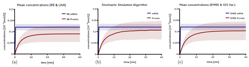
Figure 1: Gene expression model with fast transcription rate. In panels (a) and (b) we compare the RE predictions of mean concentrations with those obtained from ensemble averaging $3,000$ SSA trajectories. The shaded areas denote the region of one standard deviation around the average concentrations which in (a) has been computed using the LNA and in (b) using the SSA. For comparison, in panel (c) we show the mean concentration prediction according to the EMRE and the variance prediction according to IOS. The results in (a), (b) and (c) are in good agreement.

II-A Applications

We consider a two-stage model of gene expression with an enzymatic degradation mechanism:

$$\text{Gene}\xrightarrow{k_{0}}\text{Gene}+\text{mRNA},\ \ \text{mRNA}\xrightarrow{k_{\text{dM}}}\varnothing,$$

$$\text{mRNA}\xrightarrow{k_{s}}\text{mRNA}+\text{Protein},$$

$$\text{Protein}+\text{Enzyme}\xrightleftharpoons[k_{-1}]{k_{1}}\text{Complex}\xrightarrow{k_{2}}\text{Enzyme}+\varnothing.$$ (1)

The scheme involves the transcription of mRNA, its translation to protein and subsequent degradation of both mRNA and protein. Note that while mRNA is degraded via an unspecific linear reaction, the degradation of protein occurs via an enzyme catalyzed reaction. The latter may model proteolysis, the consumption of protein by a metabolic pathway or other post-translational modifications. A simplified version of this model is one in which the protein degradation is replaced by the linear reaction: $\text{Protein}\xrightarrow{}\varnothing$. Over the past decade the latter model has been the subject of numerous studies, principally because it can be solved exactly since the scheme is composed of purely first-order reactions [5, 6, 7]. However, the former model as given by scheme (II-A), cannot be solved exactly because of the bimolecular association reaction between enzyme and protein. Hence in what follows we demonstrate the power of approximation methods to infer useful information regarding the mechanism’s intrinsic noise properties.

We consider the model for two parameter sets (see Tab. I) at fixed compartmental volume of one femtoliter (one micron cubed). For both cases, the REs predict the same steady state mRNA and protein concentrations: $[\text{mRNA}]=0.12\mu M$ and $[\text{Protein}]=0.09\mu M$. These correspond to $72$ and $54$ molecule numbers, respectively.

We have used iNA to compute the mean concentrations using the REs and the variance of fluctuations using the LNA for parameter set (i) in which transcription is fast. Comparing these with SSA estimates (see Fig. 1) we see that the REs and LNA provide reasonably accurate results for this parameter set. This analysis was within the scope of the previous version of iNA [4]. However, the scenario considered is not particularly realistic. This is since the ratio of protein and mRNA lifetimes in this example is approximately 100 (as estimated from the time taken for the concentrations to reach $90\%$ of their steady state values) while an evaluation of 1,962 genes in budding yeast showed that the ratios have median and mode close to $3$ [7].

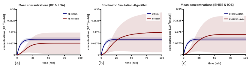
Figure 2: Gene expression model with moderate transcription rate. In panels (a) and (b) we compare the RE and LNA predictions of mean concentrations and variance of fluctuations with those obtained from ensemble averaging $30,000$ stochastic realizations computed using the SSA. Note that the RE and LNA predictions are very different than the actual values. In panel (c) we show the mean concentration prediction according to the EMRE and the variance prediction according to IOS. These are in good agreement with those obtained from the SSA.

parameter	set (i)	set (ii)
$k_{0}[G]$	$2.4\text{min}^{-1}\mu M$	$0.024\text{min}^{-1}\mu M$
$k_{\text{dM}}$	$20\text{min}^{-1}$	$0.2\text{min}^{-1}$
$k_{s}$	$1.5\text{min}^{-1}$	$1.5\text{min}^{-1}$
$k_{-1},k_{2}$	$2\text{min}^{-1}$	$2\text{min}^{-1}$
$k_{1}$	$400(\mu M\text{min})^{-1}$	$400(\mu M\text{min})^{-1}$

TABLE I: Kinetic parameters used for the gene expression model, scheme (II-A), as discussed in the main text. The volume is fixed to $\Omega=10^{-15}l$ with an enzyme concentration of $0.1\mu M$ corresponding to $60$ enzyme molecules. The Michaelis-Menten constant is $0.01\mu M$ in all cases.

We now consider parameter set (ii), the case of moderate transcription. In Fig. 2(a) and (b) we compare the RE and LNA predictions of mean concentrations and variance of fluctuations with that obtained from the SSA. Notice that in this case, the two are in severe disagreement. The SSA predicts that the mean concentration of protein is larger than that of the mRNA while the REs predict the opposite. This discreteness-induced inversion phenomenon has been described in Ref. [8]. It is also the case that the variance estimate of the LNA is considerably smaller than that of the SSA. In Fig. 2(c) we show the mean concentrations computed using the EMRE and the variance computed using the IOS method. Note that the latter are in good agreement with the SSA in Fig. 2(b). Note further that while the EMRE was already implemented in the previous version of iNA, the IOS was not. Hence the present version is the first to provide estimates of the mean concentrations and of the size of the noise which are more accurate than both the REs and the LNA. The transient times for this case are given by $37$ minutes for protein and $12$ minutes for mRNA concentrations with a ratio of approximately $3$ in agreement with the median and mode of experimentally measured ratios. Hence this example provides clear evidence of the need to go beyond the RE and LNA level of approximation for physiologically relevant parameters of the gene expression model.

II-B Implementation

iNA’s framework consist of three layers of abstraction: the SBML parser which sets up a mathematical representation of the reaction network, a module which performs the SSE analytically using the computer algebra system Ginac [9] and a just-in-time (JIT) compiler based on the LLVM [10] framework which compiles the mathematical model into platform specific machine code at runtime yielding high performance of SSE and SSA analyses implemented in iNA. Generally, methods based on the SSE require the numerical solution of a high dimensional system of linear equations. In the present version 0.3 of iNA, time-course analysis is efficiently performed by means of the all-round ODE integrator LSODA which automatically switches between explicit and implicit methods [11]. In particular, the number of simultaneous equations to be solved for the LNA, EMRE analysis is approximately proportional to $N^{2}$ where $N$ is the number of independent species after conservation analysis [12] while for IOS, the number of equations is approximately proportional to $N^{3}$. Quadratic and cubic dependencies represent a challenge for software development. iNA’s previous version 0.2 addressed this need for performance by providing a bytecode interpreter (BCI) for efficient expression evaluation [4]. The latter concept has proven its performance for both SSE and SSA methods while maintaining compatibility over many platforms. With the present version we introduce a strategy for JIT compilation based on the modern compiler framework LLVM that allows to emit and execute platform specific machine code at runtime [10]. The system size expansion ODEs are automatically compiled as native machine code making it executable directly on the CPU. Therefore iNA’s JIT feature enjoys the speed of statically compiled code while maintaining the flexibility common to interpreters. Moreover, the LLVM framework allows optimizations on platform independent and platform specific instruction levels which are beneficial for computationally expensive calculations.

Compared to iNA’s previous implementation, using JIT compilation, we have observed speedups for the SSE analysis by factors of $10-20$ and factors of $1.5-2$ for the SSA.

III Methods

We consider a general reaction network confined in a volume $\Omega$ under well-mixed conditions and involving the interaction of $N$ distinct chemical species via $R$ chemical reactions of the type

$$s_{1j}X_{1}+\ldots+s_{Nj}X_{N}\xrightarrow{k_{j}}\ r_{1j}X_{1}+\ldots+r_{Nj}X_{N},$$ (2)

where $j$ is the reaction index running from $1$ to $R$, $X_{i}$ denotes chemical species $i$, $k_{j}$ is the reaction rate of the $j^{th}$ reaction and $s_{ij}$ and $r_{ij}$ are the stoichiometric coefficients. Note that our general formulation does not require all reactions to be necessarily elementary.

The CME gives the time-evolution equation for the probability $P(\vec{n},t)$ that the system is in a particular mesoscopic state $\vec{n}=(n_{1},...,n_{N})^{T}$ where $n_{i}$ is the number of molecules of the $i^{th}$ species. It is given by:

$$\frac{\partial P(\vec{n},t)}{\partial t}=\sum_{j=1}^{R}\biggl{(}\displaystyle\prod_{i=1}^{N}E_{i}^{-S_{ij}}-1\biggr{)}\hat{a}_{j}\left(\vec{n},\Omega\right)P(\vec{n},t),$$ (3)

where $S_{ij}=r_{ij}-s_{ij}$, $\hat{a}_{j}(\vec{n},\vec{\Omega})$ is the propensity function such that the probability for the $j^{th}$ reaction to occur in the time interval $[t,t+dt)$ is given by $\hat{a}_{j}(\vec{n},\vec{\Omega})dt$ [3] and $E_{i}^{-S_{ij}}$ is the step operator defined by its action on a general function of molecular populations as $E_{i}^{-S_{ij}}g(n_{1},...,n_{i},...,n_{N})=g(n_{1},...,n_{i}-S_{ij},...,n_{N})$ [2].

The CME is typically intractable for computational purposes because of the inherently large state space. iNA circumvents this problem by approximating the moments of probability density solution of the CME systematically using van Kampen’s SSE [2, 13]. The starting point of the analysis is van Kampen’s ansatz

$$\frac{\vec{n}}{\Omega}=[\vec{X}]+\Omega^{-1/2}\vec{\epsilon},$$ (4)

by which one separates the instantaneous concentration into a deterministic part given by the solution $[\vec{X}]$ of the macroscopic REs for the reaction scheme (2) and the fluctuations around it parametrized by $\vec{\epsilon}$. The change of variable causes the probability distribution of molecular populations $P(\vec{n},t)$ to be transformed into a new probability distribution of fluctuations $\Pi(\vec{\epsilon},t)$. The time derivative, the step operator and the propensity functions are also transformed (see [4] for details). In particular, using ansatz (4) together with the explicit $\Omega$-dependence of the propensities as given by ${\hat{a}_{j}(\vec{n},\Omega)}=\sum_{m=0}^{\infty}\Omega^{1-m}f_{j}^{(m)}(\frac{\vec{n}}{\Omega})$, the propensities can be expanded in powers of $\Omega^{-1/2}$:

$$\frac{\hat{a}_{j}(\vec{n},\Omega)}{\Omega}= f_{j}^{(0)}([\vec{X}])+\Omega^{-1/2}\epsilon_{\alpha}\frac{\partial f_{j}^{(0)}([\vec{X}])}{\partial{[{X}_{\alpha}]}}+\Omega^{-1}f_{j}^{(1)}([\vec{X}])$$

$$+\frac{1}{2}\Omega^{-1}\epsilon_{\alpha}\epsilon_{\beta}\frac{\partial f_{j}^{(0)}([\vec{X}])}{\partial{[X_{\alpha}]}\partial[X_{\beta}]}+\Omega^{-3/2}\epsilon_{\alpha}\frac{\partial f_{j}^{(1)}([\vec{X}])}{\partial{[{X}_{\alpha}]}}$$

$$+\frac{1}{2}\Omega^{-3/2}\epsilon_{\alpha}\epsilon_{\beta}\epsilon_{\gamma}\frac{\partial f_{j}^{(0)}([\vec{X}])}{\partial{[X_{\alpha}]}\partial[X_{\beta}]\partial{[X_{\gamma}]}}+O(\Omega^{-2}).$$ (5)

Note that $\vec{f}^{(0)}$ is the macroscopic rate function. Here we have used the convention that twice repeated Greek indices are summed over 1 to $N$, which we use in what follows as well. Consequently the CME up to order $\Omega^{-1}$ can be written as

$$\frac{\partial\Pi(\vec{\epsilon},t)}{\partial t}-\Omega^{1/2}\left(\frac{\partial[X_{\alpha}]}{\partial t}-\sum_{k=1}^{R}S_{\alpha k}f_{k}^{(0)}([\vec{X}])\right){\partial_{\alpha}\Pi(\vec{\epsilon},t)}$$

$$\qquad=\left(\Omega^{0}\mathcal{L}^{(0)}+\Omega^{-1/2}\mathcal{L}^{(1)}+\Omega^{-1}\mathcal{L}^{(2)}\right)\,\Pi(\vec{\epsilon},t)$$

$$\qquad\qquad+O(\Omega^{-3/2}),$$ (6)

where the operators are defined as

$$\mathcal{L}^{(0)} =-\partial_{\alpha}{J}_{\alpha}^{\beta}\epsilon_{\beta}+\frac{1}{2}\partial_{\alpha}\partial_{\beta}D_{\alpha\beta},$$

$$\mathcal{L}^{(1)} =-\partial_{\alpha}{D}_{\alpha}^{(1)}-\frac{1}{2!}\partial_{\alpha}{J}_{\alpha}^{\beta\gamma}\epsilon_{\beta}\epsilon_{\gamma}+\frac{1}{2!}\partial_{\alpha}\partial_{\beta}{J}_{\alpha\beta}^{\gamma}\epsilon_{\gamma}$$

$$-\frac{1}{3!}\partial_{\alpha}\partial_{\beta}\partial_{\gamma}{D}_{\alpha\beta\gamma},$$

$$\mathcal{L}^{(2)} =-\partial_{\alpha}J^{(1)\beta}_{\alpha}\epsilon_{\beta}+\frac{1}{2!}\partial_{\alpha}\partial_{\beta}{D}^{(1)}_{\alpha\beta}-\frac{1}{3!}\partial_{\alpha}{J}_{\alpha}^{\beta\gamma\delta}\epsilon_{\beta}\epsilon_{\gamma}\epsilon_{\delta}$$

$$+\frac{1}{2!}\frac{1}{2!}\partial_{\alpha}\partial_{\beta}{J}_{\alpha\beta}^{\gamma\delta}\epsilon_{\gamma}\epsilon_{\delta}-\frac{1}{3!}\partial_{\alpha}\partial_{\beta}\partial_{\gamma}{J}_{\alpha\beta\gamma}^{\delta}\epsilon_{\delta}$$

$$+\frac{1}{4!}\partial_{\alpha}\partial_{\beta}\partial_{\gamma}\partial_{\delta}{D}_{\alpha\beta\gamma\delta},$$ (7)

and the SSE coefficients are given by

$${D^{(n)}}_{ij..r} =\sum\limits_{k=1}^{R}S_{ik}S_{jk}...S_{rk}\,{f}^{(n)}_{k}([\vec{X}]),$$

$${J^{(n)}}_{ij..r}^{st..z} =\frac{\partial}{\partial{[X_{s}]}}\frac{\partial}{\partial{[X_{t}]}}...\frac{\partial}{\partial{[X_{z}]}}{D^{(n)}}_{ij..r}.$$ (8)

Note that the above expressions generalize the expansion carried out in Ref. [14] to include also non-elementary reactions as for instance trimolecular reactions or reactions with propensities of the Michaelis-Menten type [15]. Note also that the $\Omega^{1/2}$ term vanishes since the macroscopic REs are given by $\partial_{t}[X_{\alpha}]=\sum_{k=1}^{R}S_{\alpha k}f_{k}^{(0)}([\vec{X}])$ leaving us with a series expansion of the CME in powers of the inverse square root of the volume. In Eqs. (III) we have omitted the upper index in the bracket of the SSE coefficients in the case of $n=0$.

The method now proceeds by constructing equations for the moments of the $\vec{\epsilon}$ variables. This is accomplished by expanding the probability distribution of fluctuations $\Pi(\vec{\epsilon},t)$ in terms of the inverse square root of the volume as $\Pi(\vec{\epsilon},t)=\sum_{j=0}^{\infty}\Pi_{j}(\vec{\epsilon},t)\Omega^{-j/2}$, which implies an equivalent expansion of the moments

$$\langle\epsilon_{k}\epsilon_{l}...\epsilon_{m}\rangle=\sum_{j=0}^{\infty}[\epsilon_{k}\epsilon_{l}...\epsilon_{m}]_{j}\Omega^{-j/2}.$$ (9)

In order to relate the above moments back to the moments of the concentration variables we use Eqs. (4) and (9) to find expressions for the mean concentrations and covariance of fluctuations which are given by

$$\left\langle\frac{n_{i}}{\Omega}\right\rangle =\,[X_{i}]+{\Omega}^{-1}\left[\epsilon_{i}\right]_{1}+O(\Omega^{-2}),$$ (10a)

$$\Sigma_{ij} =\,\left\langle\left(\frac{n_{i}}{\Omega}-\left\langle\frac{n_{i}}{\Omega}\right\rangle\right)\left(\frac{n_{j}}{\Omega}-\left\langle\frac{n_{j}}{\Omega}\right\rangle\right)\right\rangle$$

$$=\,\Omega^{-1}\left[\epsilon_{i}\epsilon_{j}\right]_{0}+\Omega^{-2}\left(\left[\epsilon_{i}\epsilon_{j}\right]_{2}-\left[\epsilon_{i}\right]_{1}\left[\epsilon_{j}\right]_{1}\right)$$

$$\qquad+O(\Omega^{-3})$$ (10b)

The order $\Omega^{0}$ term of Eq. (10a) denotes the mean concentrations as given by the macroscopic REs while the $\Omega^{-1}$ term in Eq. (10b) gives the LNA estimate for the covariance. Including terms to order $\Omega^{-1}$ in Eq. (10a) gives the EMRE estimate of the mean concentrations which corrects the estimate of the REs. Finally, considering also the $\Omega^{-2}$ term in Eq. (10b) gives the IOS (Inverse Omega Squared) estimate of the variance which is centered around the EMRE concentrations and is of higher accuracy than the LNA method. The general procedure together with the equations determining the coefficients of Eq. (9) is presented in Refs. [14] and [16]. In brief the result can be summarized as follows: as mentioned above, truncating Eq. (III) to order $\Omega^{1/2}$ yields the macroscopic REs, truncation after terms up to order $\Omega^{0}$ gives a Fokker-Planck equation with linear drift and diffusion coefficients which is also called the Linear Noise Approximation. Considering terms up to $\Omega^{-1/2}$ one obtains the EMREs while the terms up to $\Omega^{-1}$ determine the corrections beyond the LNA as given by the present IOS method. Since the IOS method has been derived from van Kampen’s ansatz, Eq. (4), which expands the CME around the macroscopic concentrations it has the same limitation as the LNA namely that it cannot account for systems exhibiting bistability.

IV Discussion

In this proceeding we have introduced and implemented the IOS approximation in the software package iNA. This allows the variances to be determined accurate to order $\Omega^{-2}$, an approximation which complements the EMRE method (mean concentrations accurate to order $\Omega^{-1}$) and is superior to the previously implemented LNA method (variances accurate to order $\Omega^{0}$). As we have shown this increased accuracy is desirable to accurately account for the effects of intrinsic noise in biochemical reaction networks under low molecule number conditions. In particular, we have demonstrated the utility of the software by analyzing an example of gene expression with a functional enzyme. We have also extended iNA by a more efficient JIT compilation strategy in combination with improved numerical algorithms which offers high performance and enables computations feasible even on desktop PCs. This feature is particularly important when analyzing noise in reaction networks of intermediate or large size with bimolecular reactions, conditions that have been shown to amplify the deviations from the conventional rate equation description [17].

Availability

The software iNA version 0.3 is freely available under http://code.google.com/p/intrinsic-noise-analyzer/ as executable binaries for Linux, MacOSX and Microsoft Windows, as well as the full source code under an open source license.

References

- [1] Y. Ishihama, T. Schmidt, J. Rappsilber, M. Mann, U. Hartl, M. J. Kerner, and D. Frishman. Protein abundance profiling of the escherichia coli cytosol. BMC Genomics, 9:102, 2008.
- [2] N.G. van Kampen. Stochastic processes in physics and chemistry. North-Holland, 3rd edition, 2007.
- [3] D.T. Gillespie. Stochastic simulation of chemical kinetics. Annu. Rev. Phys. Chem., 58:35–55, 2007.
- [4] P. Thomas, H. Matuschek, and R. Grima. Intrinsic noise analyzer: A software package for the exploration of stochastic biochemical kinetics using the system size expansion. PloS one, 7(6):e38518, 2012.
- [5] E.M. Ozbudak, M. Thattai, I. Kurtser, A.D. Grossman, and A. van Oudenaarden. Regulation of noise in the expression of a single gene. Nature genetics, 31(1):69–73, 2002.
- [6] J. Paulsson. Models of stochastic gene expression. Physics of life reviews, 2(2):157–175, 2005.
- [7] V. Shahrezaei and P.S. Swain. Analytical distributions for stochastic gene expression. Proceedings of the National Academy of Sciences, 105(45):17256, 2008.
- [8] R. Ramaswamy, N. González-Segredo, I.F. Sbalzarini, and R. Grima. Discreteness-induced concentration inversion in mesoscopic chemical systems. Nature Communications, 3:779, 2012.
- [9] C. Bauer, A. Frink, and R. Kreckel. Introduction to the ginac framework for symbolic computation within the C++ programming language. Journal of Symbolic Computation, 33(1):1–12, 2002.
- [10] C. Lattner and V. Adve. LLVM: A compilation framework for lifelong program analysis & transformation. In Code Generation and Optimization, 2004. CGO 2004. International Symposium on, pages 75–86. IEEE, 2004.
- [11] L. Petzold. Automatic selection of methods for solving stiff and nonstiff systems of ordinary differential equations. SIAM Journal on Scientific and Statistical Computing, 4(1):136–148, 1983.
- [12] R.R. Vallabhajosyula, V. Chickarmane, and H.M. Sauro. Conservation analysis of large biochemical networks. Bioinformatics, 22(3):346–353, 2006.
- [13] NG Van Kampen. The expansion of the master equation. Advances in Chemical Physics, pages 245–309, 1976.
- [14] R. Grima, P. Thomas, and A.V. Straube. How accurate are the nonlinear chemical fokker-planck and chemical langevin equations? The Journal of Chemical Physics, 135:084103, 2011.
- [15] C.V. Rao and A.P. Arkin. Stochastic chemical kinetics and the quasi-steady-state assumption: Application to the gillespie algorithm. The Journal of chemical physics, 118:4999, 2003.
- [16] R. Grima. A study of the accuracy of moment-closure approximations for stochastic chemical kinetics. The Journal of Chemical Physics, 136:154105, 2012.
- [17] P. Thomas, A.V. Straube, and R. Grima. Stochastic theory of large-scale enzyme-reaction networks: Finite copy number corrections to rate equation models. Journal of Chemical Physics, 133(19):195101, 2010.