The Smile of certain Lévy-type Models

Abstract

We consider a class of assets whose risk-neutral pricing dynamics are described by an exponential Lévy-type process subject to default. The class of processes we consider features locally-dependent drift, diffusion and default-intensity as well as a locally-dependent Lévy measure. Using techniques from regular perturbation theory and Fourier analysis, we derive a series expansion for the price of a European-style option. We also provide precise conditions under which this series expansion converges to the exact price. Additionally, for a certain subclass of assets in our modeling framework, we derive an expansion for the implied volatility induced by our option pricing formula. The implied volatility expansion is exact within its radius of convergence. As an example of our framework, we propose a class of CEV-like Lévy-type models. Within this class, approximate option prices can be computed by a single Fourier integral and approximate implied volatilities are explicit (i.e., no integration is required). Furthermore, the class of CEV-like Lévy-type models is shown to provide a tight fit to the implied volatility surface of S&P500 index options.

Keywords Regular Perturbation, Lévy-type, Local Volatility, Implied Volatility, Default, CEV

1 Introduction

A local volatility model is a model in which the volatility $\sigma_{t}$ of an asset $X$ is a function of the current time $t$ and the present level of $X$. That is, $\sigma_{t}=\sigma(t,X_{t})$. One advantage of local volatility models is that, like most scalar diffusions, transition densities (and therefore option prices) are often available in closed-form as eigenfunction expansions (see Linetsky (2007); Lipton (2002a) and references therein). However, local volatility models suffer from the fact that they do not permit the underlying asset to experience jumps, the need for which is well-documented in literature Eraker (2004). Furthermore, local volatility models do not account properly for the forward volatility, and notoriously misprice options such as cliquet or forward-start.

One class of models that does allow the underlying to jump is the exponential Lévy class. In this class, the underlying $X=e^{Y}$ is described as the exponential of a Lévy process $Y$. Aside from allowing the underlying to jump, exponential Lévy models have the desirable feature that transition densities (and European option prices) can be computed quickly as generalized Fourier transforms (see Lewis (2001); Lipton (2002b); Boyarchenko and Levendorskii (2002); Cont and Tankov (2004)). However, exponential Lévy models are spatially homogeneous; neither the drift, volatility nor the jump-intensity have any local dependence. Thus, exponential Lévy models are not able to exhibit volatility clustering or capture the leverage effect, both of which are well-known features of equity markets.

Recently, a number of authors have found methods of combining the desirable features of local volatility and exponential Lévy models. For example, Benhamou, Gobet, and Miri (2009) derive an analytical formula for the approximate prices of European options, for models that include local volatility and compound Poisson jumps (i.e., models that include a finite activity Lévy measure). Their approach relies on asymptotic expansions around small diffusion and small jump frequency/size limits. More recently, Pagliarani, Pascucci, and Candia (2011) consider general local volatility models with independent Lévy jumps (not necessarily finite activity). Unlike, Benhamou et al. (2009), Pagliarani et al. (2011) make no small jump intensity/size assumption. Rather the authors construct an asymptotic solution of the pricing equation by expanding the local volatility function as a Taylor series. While both of the methods described above allow for local volatility and independent jumps, neither of these methods allow for state-dependent jumps.

Stochastic jump-intensity is an important feature of equity markets (see Christoffersen, Jacobs, and Ornthanalai (2009)) and a locally dependent Lévy measure is one way to incorporate stochastic jump-intensity into a modeling framework. One analytically tractable way of obtaining a local Lévy measure is to time-change a scalar Markov diffusion with a Lévy subordinator, as described in Mendoza-Arriaga, Carr, and Linetsky (2010). Another analytically tractable method of working with local Lévy measures is to write a local Lévy measure as a power series in its local variable, as described in Lorig, Pagliarani, and Pascucci (2013).

In this paper, we take a different approach. We consider a Lévy-type process whose infinitesimal generator separates into locally dependent and independent parts. The locally independent part is the generator of a Lévy process with killing. We treat the locally dependent part of the generator as a regular perturbation about the locally independent part. Thus, we are able to obtain a convergent series representation for the price of a European option. A significant advantage of this method is that, when the locally independent part of the generator has no jump or killing component, we are able find a convergent series expansion for the implied volatility surface induced by our option pricing formula.

The rest of this paper proceeds as follows: In Section 2, we present a class of exponential Lévy-type models and state our assumptions about the market. In Section 3, using regular perturbation methods and Fourier analysis, we derive a series expansion for the price of a European option. We also provide precise conditions under which this series converges to give the exact option price. In Section 4, we provide a series expansion for the implied volatility smile induced by a certain sub-class of models within our modeling framework. This series is exact within its radius of convergence. In Section 5, we perform specific computations for a class of CEV-like Lévy-type model. In this class, approximate option prices can be computed by a single Fourier integral; approximate implied volatilities are explicit, requiring no integration. Section 5 also includes extensive numerical examples, including a calibration to S&P500 options. Proofs and some sample Mathematica code can be found in an Appendix. Lastly, some concluding remarks are given in Section 6.

2 Model and assumptions

We assume a frictionless market, no arbitrage and take an equivalent martingale measure $\mathbb{P}$ to be chosen by the market on a complete filtered probability space $(\Omega,\mathscr{F},\{\mathscr{F}_{t},t\geq 0\},\mathbb{P})$. The filtration $\{\mathscr{F}_{t},t\geq 0\}$ represents the history of the market. All processes defined below live on this space. For simplicity, we assume zero interest rates and no dividends. Thus, in the absence of arbitrage, all traded assets are martingales. We consider a risky asset $X$, whose dynamics are given by

$$X_{t} =\mathbb{I}_{\{t<\zeta\}}\exp(Y_{t}),$$ (1)

$$dY_{t} =\alpha(Y_{t})dt+\sigma(Y_{t})dW_{t}+\int_{\mathbb{R}}zd\widetilde{N}_{t}(Y_{t-},dz), Y_{0} =y\in\mathbb{R},$$ (2)

$$\zeta =\inf\left\{t\geq 0:\int_{0}^{t}k(Y_{s})ds=\mathscr{E}\right\}, \mathscr{E} \sim\text{Exp}(1),$$ (3)

where $W$ is a Brownian motion, $\mathscr{E}$ is an independent exponentially distributed random variable with parameter one, and $d\widetilde{N}_{t}(Y_{t-},dz)$ is a state-dependent compensated Poisson random measure

$$d\widetilde{N}_{t}(Y_{t-},dz) =dN_{t}(Y_{t-},dz)-\nu(Y_{t-},dz), \mathbb{E}[dN_{t}(Y_{t-},dz)|Y_{t-}] =\nu(Y_{t-},dz)dt.$$ (4)

The volatility, killing, and drift functions, as well as the state-dependent Lévy measure are given by

$$\sigma(y) =\Big{(}a_{0}^{2}+\varepsilon a_{1}^{2}\eta(y)\Big{)}^{1/2},$$ (5)

$$k(y) =c_{0}+\varepsilon c_{1}\eta(y),$$ (6)

$$\nu(y,dz) =\nu_{0}(dz)+\varepsilon\eta(y)\nu_{1}(dz),$$ (7)

$$\alpha(y) =k(y)-\frac{1}{2}\sigma^{2}(y)-\int_{\mathbb{R}}\nu(y,dz)\Big{(}e^{z}-1-z\Big{)}.$$ (8)

Here, $(a_{0},a_{1},c_{0},c_{1},\varepsilon)$ are non-negative constants and the function $\eta$ belongs to $\mathscr{S}$, the Schwartz space of rapidly decreasing functions on $\mathbb{R}$:

$$\mathscr{S} =\{f\in C^{\infty}(\mathbb{R}):\left\|{f}\right\|_{\alpha,\beta}<\infty,\ \text{for all }(\alpha,\beta)\in\mathbb{N}^{2}\}, \left\|{f}\right\|_{\alpha,\beta} :=\sup_{y\in\mathbb{R}}|y^{\alpha}\partial^{\beta}f(y)|.$$ (9)

The function $\eta$ must be such that $\sigma(y)>0$, $k(y)\geq 0$ and $\nu(y,A)\geq 0$ for all $y\in\mathbb{R}$ and all Borel sets $A$. Finally, we assume that the locally-dependent Lévy measure $\nu(y,dz)$ satisfies, for any $y\in\mathbb{R}$,

$$\int_{\mathbb{R}}\min(1,z^{2})\nu(y,dz)<\infty,\qquad\nu(y,\{0\})=0,$$ (10)

$$\int_{|z|\geq 1}e^{z}\nu(y,dz)<\infty,\qquad\int_{|z|\geq 1}|z|\nu(y,dz)<\infty.$$ (11)

Conditions (10) are part of the definition of a Lévy measure while the conditions (11) relate to the existence of moments greater than one, see in particular item 4 below. Note further that these three conditions also hold for both $\nu_{0}$ and $\nu_{1}$. We denote by $\mathscr{F}_{t}^{Y}$ the filtration generated by $Y$. Note that $\zeta$, which represents the default time of $X$, is not $\mathscr{F}_{t}^{Y}$-measurable. Thus, we introduce an indicator process $D_{t}:=\mathbb{I}_{\{\zeta\leq t\}}$ in order to keep track of the event $\{\zeta\leq t\}$. We denote by $\mathscr{F}_{t}^{D}$ the filtration generated by $D$. The filtration of a market observer, then, is $\mathscr{F}_{t}=\mathscr{F}_{t}^{Y}\vee\mathscr{F}_{t}^{D}$. The main features of the class of models described above are as follows:

1. Local volatility: the process $Y$ has a local volatility component: $\sigma(y)=\left(a_{0}^{2}+\varepsilon a_{1}^{2}\eta(y)\right)^{1/2}$.

2. Local Lévy measure: jumps in $Y$ of size $dz$ arrive with a state-dependent intensity described by the local Lévy measure $\nu(y,dz)$. The Lévy measure has the decomposition $\nu(y,dz)=\nu_{0}(dz)+\varepsilon\eta(y)\nu_{1}(dz)$, where $\nu_{0}$ and $\nu_{1}$ are both Lévy measures. Note that both the jump intensity and the jump distribution can change depending on the value of $y$.

3. Local default intensity: the underlying asset $X$ can default (i.e., for any $t>0$, $\mathbb{P}(X_{t}=0)>0$) with a state-dependent default intensity of $k(y):=c_{0}+\varepsilon c_{1}\eta(y)$.

4. Martingale: the conditions above ensure that $\mathbb{E}(X_{t})$ is finite for any $t\geq 0$. The drift function $\alpha$ is fixed by the Lévy measure, the volatility and the killing functions, ensuring that $X$ is a martingale.

5. Existence: the Lévy-Itô SDE (2) has a unique strong solution (see Theorem 1.19 in Øksendal and Sulem (2005)).

3 Option pricing

Let $V_{t}$ be the value at time $t$ of a European derivative, expiring at time $T>t$ with payoff $H(X_{T})$. For convenience, we introduce the function $h:\mathbb{R}\ni y\mapsto H(e^{y})$ with $K:=H(0)$. Using risk-neutral pricing, $V_{t}$ is expressed as the conditional expectation of the option payoff

$$V_{t} =\mathbb{E}\left[H(X_{T})|\mathscr{F}_{t}\right]$$ (12)

$$=\mathbb{E}\left[h(Y_{T})\mathbb{I}_{\{\zeta>T\}}|\mathscr{F}_{t}\right]+K\mathbb{E}\left[\mathbb{I}_{\{\zeta\leq T\}}|\mathscr{F}_{t}\right]$$ (13)

$$=\mathbb{E}\left[h(Y_{T})\mathbb{I}_{\{\zeta>T\}}|\mathscr{F}_{t}\right]+K-K\mathbb{E}\left[\mathbb{I}_{\{\zeta>T\}}|\mathscr{F}_{t}\right]$$ (14)

$$=\mathbb{I}_{\{\zeta>t\}}\mathbb{E}\left[h(Y_{T})e^{-\int_{t}^{T}k(Y_{s})ds}|\mathscr{F}_{t}^{Y}\right]+K-K\mathbb{I}_{\{\zeta>t\}}\mathbb{E}\left[e^{-\int_{t}^{T}k(Y_{s})ds}|\mathscr{F}_{t}^{Y}\right]$$ (15)

$$=\mathbb{I}_{\{\zeta>t\}}\mathbb{E}\left[h(Y_{T})e^{-\int_{t}^{T}k(Y_{s})ds}|Y_{t}\right]+K-K\mathbb{I}_{\{\zeta>t\}}\mathbb{E}\left[e^{-\int_{t}^{T}k(Y_{s})ds}|Y_{t}\right],$$ (16)

where we have used

$$\mathbb{E}\left[h(Y_{T})\mathbb{I}_{\{\zeta>T\}}|\mathscr{F}_{t}\right] =\mathbb{I}_{\{\zeta>T\}}\mathbb{E}\left[h(Y_{T})\mathbb{E}[\mathbb{I}_{\{\zeta>T\}}|\mathscr{F}_{T}^{Y}\vee\mathscr{F}_{t}]|\mathscr{F}_{t}\right]$$ (17)

$$=\mathbb{I}_{\{\zeta>T\}}\mathbb{E}\left[h(Y_{T})e^{-\int_{t}^{T}k(Y_{s})ds}|\mathscr{F}_{t}\right]$$ (18)

$$=\mathbb{I}_{\{\zeta>T\}}\mathbb{E}\left[h(Y_{T})e^{-\int_{t}^{T}k(Y_{s})ds}|\mathscr{F}_{t}^{Y}\right].$$ (19)

Using the time-homogeneity of $Y$, it is clear that

$$\mathbb{E}\left[h(Y_{T})e^{-\int_{t}^{T}k(Y_{s})ds}|Y_{t}=y\right]=\mathbb{E}_{y}\left[h(Y_{T-t})e^{-\int_{0}^{T-t}k(Y_{s})ds}\right],$$

where the notation $\mathbb{E}_{y}$ means $\mathbb{E}[\cdot|Y_{0}=y]$. Thus, to value a European-style derivative, we must compute expectations of the form

$$u^{\varepsilon}(t,y):=\mathbb{E}_{y}\left[h(Y_{t})e^{-\int_{0}^{t}k(Y_{s})ds}\right].$$ (20)

We explicitly indicate the dependence of $u^{\varepsilon}(t,y)$ on the parameter $\varepsilon$, which will play a key role in the regular perturbation analysis below. The function $u^{\varepsilon}(t,y)$ in (20) satisfies the Kolmogorov backward equation

$$\left(-\partial_{t}+\mathscr{A}^{\varepsilon}\right)u^{\varepsilon} =0, \text{with boundary condition }u^{\varepsilon}(0,y)=h(y),$$ (21)

where the infinitesimal generator $\mathscr{A}^{\varepsilon}$ is defined by

$$\mathscr{A}^{\varepsilon}f(x)=\lim_{t\to 0^{+}}\frac{1}{t}\left(\mathbb{E}_{y}\left[f(Y_{t})e^{-\int_{0}^{t}k(Y_{s})ds}\right]-f(y)\right),\qquad\text{whenever the limit exists}.$$ (22)

If $f\in C_{0}^{2}(\mathbb{R})$, then the limit (22) does exist and the generator $\mathscr{A}^{\varepsilon}$ has the explicit representation

$$\mathscr{A}^{\varepsilon} =\mathscr{A}_{0}+\varepsilon\eta\mathscr{A}_{1},$$ (23)

$$\mathscr{A}_{i} =\frac{1}{2}a_{i}^{2}\left(\partial^{2}-\partial\right)+c_{i}\left(\partial-1\right)-\int_{\mathbb{R}}\nu_{i}(dz)\Big{(}e^{z}-1-z\Big{)}\partial+\int_{\mathbb{R}}\nu_{i}(dz)\Big{(}\theta_{z}-1-z\partial\Big{)}, i \in\{0,1\},$$ (24)

where $\partial$ (without the subscript $t$) indicates differentiation with respect to $y$ and $\theta_{z}$ is the shift operator: $\theta_{z}f(y)=f(y+z)$. We define ${\rm dom}(\mathscr{A}^{\varepsilon})$ as the set of functions $u$ such that the derivatives and integrals appearing in $\mathscr{A}^{\varepsilon}u$ with $\mathscr{A}^{\varepsilon}$ given by (23)-(24) exist and are finite.

Remark 1.

By Jacod and Shiryaev (1987), Definition II.8.25, Proposition II.8.26, the operators $\mathscr{A}_{0}$ and $\mathscr{A}_{1}$ correspond to infinitesimal generators of Lévy processes which are exponentially special semimartingales.

Assumption 2.

We assume the existence of a unique classical solution to the Cauchy problem (21). A sufficient (but not necessary) condition for its existence is that the payoff function $h$ and its first two derivatives are bounded (see Theorem 3.2, Chapter 3 in Bensoussan and Lions (1984)).

From (23), since the operator $\mathscr{A}^{\varepsilon}$ decomposes into $\mathscr{O}(1)$ and $\mathscr{O}(\varepsilon)$ terms, we seek a solution to the Cauchy problem (21) of the form

$$u^{\varepsilon} =\sum_{n=0}^{\infty}\varepsilon^{n}u_{n}.$$ (25)

Conditions under which this expansion is valid will be given in Theorem 4. Inserting the expansion (25) into the Cauchy problem (21) and collecting terms of like powers of $\varepsilon$ we find

$$\mathscr{O}(1): (-\partial_{t}+\mathscr{A}_{0})u_{0} =0, u_{0}(0,y) =h(y),$$ (26)

$$\mathscr{O}(\varepsilon^{n}): (-\partial_{t}+\mathscr{A}_{0})u_{n} =-\eta\mathscr{A}_{1}u_{n-1}, u_{n}(0,y) =0, \text{for }n\geq 1.$$ (27)

To solve the above Cauchy problems, it will be convenient to introduce the notations

$$\langle u,v\rangle:=\int_{\mathbb{R}}\overline{u(y)}v(y)dy\qquad\text{and}\qquad\left\|{u}\right\|^{2}:=\langle u,u\rangle.$$ (28)

Note that the inner product $\langle u,v\rangle$ may be infinite. We also introduce $\mathscr{A}^{*}_{i}$, the formal adjoint of $\mathscr{A}_{i}$ defined via the relation $\langle u,\mathscr{A}_{i}v\rangle=\langle\mathscr{A}^{*}_{i}u,v\rangle$, for any Schwartz functions $u$ and $v$. Explicitly, $\mathscr{A}^{*}_{i}$ is given by

$$\mathscr{A}^{*}_{i}=\frac{1}{2}a_{i}^{2}\left(\partial^{2}+\partial\right)+c_{i}\left(-\partial-1\right)+\int_{\mathbb{R}}\nu_{i}(dz)\left(e^{z}-1-z\right)\partial+\int_{\mathbb{R}}\nu_{i}(dz)(\theta_{-z}-1+z\partial),$$ (29)

for $i=0,1$, which can be deduced through integrating by parts. We note the following important relations

$$\mathscr{A}_{0}\psi_{\lambda} =\phi_{\lambda}\psi_{\lambda}, \mathscr{A}^{*}_{0}\overline{\psi_{\lambda}} =\phi_{\lambda}\overline{\psi_{\lambda}}, \mathscr{A}_{1}\psi_{\lambda} =\chi_{\lambda}\psi_{\lambda}, \mathscr{A}^{*}_{1}\overline{\psi_{\lambda}} =\chi_{\lambda}\overline{\psi_{\lambda}},$$ (30)

where

$$\psi_{\lambda}(y) :=\frac{1}{\sqrt{2\pi}}e^{i\lambda y},$$ (31)

$$\phi_{\lambda} :=\frac{1}{2}a_{0}^{2}\left(-\lambda^{2}-i\lambda\right)+c_{0}(i\lambda-1)-\int_{\mathbb{R}}\nu_{0}(dz)\Big{(}e^{z}-1-z\Big{)}i\lambda+\int_{\mathbb{R}}\nu_{0}(dz)\Big{(}e^{i\lambda z}-1-i\lambda z\Big{)},$$ (32)

$$\chi_{\lambda} :=\frac{1}{2}a_{1}^{2}\left(-\lambda^{2}-i\lambda\right)+c_{1}(i\lambda-1)-\int_{\mathbb{R}}\nu_{1}(dz)\Big{(}e^{z}-1-z\Big{)}i\lambda+\int_{\mathbb{R}}\nu_{1}(dz)\Big{(}e^{i\lambda z}-1-i\lambda z\Big{)}.$$ (33)

Note that for any function $u$ and any complex number $\lambda:=\lambda_{r}+i\lambda_{i}\in\mathbb{C}$ such that $\langle\psi_{\lambda},u\rangle$ is finite, we have the generalized Fourier representation

$$u(y)=\int_{\mathbb{R}}d\lambda_{r}\langle\psi_{\lambda},u\rangle\psi_{\lambda}(y).$$ (34)

However, whenever $u\in L^{2}(\mathbb{R})$, such a generalized representation is not necessary, and the simpler form (with $\lambda\in\mathbb{R}$) $u(y)=\int_{\mathbb{R}}d\lambda\langle\psi_{\lambda},u\rangle\psi_{\lambda}(y)$ suffices. We are now in a position to find an explicit solution to (26)-(27).

Proposition 3.

Suppose that $u_{0}$ satisfies (26). Then the sequence $(u_{n})$ defined in (27) reads

$$u_{n}(t,y) =\underbrace{\int_{\mathbb{R}}\cdots\int_{\mathbb{R}}}_{n+1}\left(\prod_{k=0}^{n}d\lambda_{k}\right)\left(\sum_{k=0}^{n}\frac{e^{t\phi_{\lambda_{k}}}}{\prod_{j\neq k}^{n}(\phi_{\lambda_{k}}-\phi_{\lambda_{j}})}\right)\left(\prod_{k=0}^{n-1}\chi_{\lambda_{k}}\langle\psi_{\lambda_{k+1}},\eta\psi_{\lambda_{k}}\rangle\right)\langle\psi_{\lambda_{0}},h\rangle\psi_{\lambda_{n}}(y),$$ (35)

where $\prod_{k=0}^{-1}(\cdots)=1$ and $\prod_{j\neq k}^{0}(\cdots)=1$ by convention.

Proof.

See Appendix A. ∎

We have obtained a formal expansion ((25) and (35)) for $u^{\varepsilon}$. The following theorem provides precise conditions under which the expansion is guaranteed to be valid. From now on, we shall denote by $L^{2}(\mathbb{R})$ the set of all real functions which are square integrable with respect to the Lebesgue measure.

Theorem 4.

Suppose $h\in L^{2}(\mathbb{R})\cap{\rm dom}(\mathscr{A}^{\varepsilon})$. Suppose further that for any $u\in L^{2}(\mathbb{R})$

$$\int_{\mathbb{R}}d\lambda|\phi_{\lambda}|^{2}|\langle\psi_{\lambda},u\rangle|^{2}<\infty \qquad\text{implies}\qquad\int_{\mathbb{R}}d\lambda|\chi_{\lambda}|^{2}|\langle\psi_{\lambda},u\rangle|^{2}<\infty,$$ (36)

and that there exist two real constants $A\geq 0$ and $B\leq 1$ (independent of $(t,y)$) such that

$$\varepsilon^{2} \leq\inf_{\lambda\in\mathbb{R}}\frac{A^{2}+B^{2}|\phi_{\lambda}|^{2}}{\left\|\eta\right\|^{2}\cdot|\chi_{\lambda}|^{2}}.$$ (37)

Then the option price $u^{\varepsilon}(t,y)$ is an analytic function of $\varepsilon$ and its power series expansion is given by (25) where the sequence $\{u_{n}\}_{n=0}^{\infty}$ is given by (35). The sequence of partial sums $u^{(N)}(t,y):=\sum_{n=0}^{N}\varepsilon^{n}u_{n}(t,y)$ converges uniformly (with respect to $\varepsilon$) to the exact price $u^{\varepsilon}(t,y)$.

Proof.

See Appendix B. The last convergence statement simply follows from the fact that every power series converges uniformly within its radius of convergence. ∎

Remark 5.

We wish to rectify a common misperception. Under the conditions of Theorem 4, the series expansion (25) is the exact option price $u^{\varepsilon}(t,y)$. It is not an asymptotic approximation.

Remark 6 (Feynman-Kac transition densities).

Since the diffusion component $\sigma$ of $Y$ is non-zero, as assumed in Section 2, the function $u^{\varepsilon}(t,y)$ can be written as an integral with respect to a density

$$u^{\varepsilon}(t,y) :=\mathbb{E}_{y}\left(h(Y_{t})e^{-\int_{0}^{t}k(Y_{s})ds}\right)=\int_{\mathbb{R}}h(z)p^{\varepsilon}(t,y,z)dz.$$ (38)

The density $p^{\varepsilon}(t,y,z)$ is called the Feynman-Kac (FK) transition density. However it is not a probability density since, due to the killing function $k(y)$, it is norm-defecting, i.e. $\int_{\mathbb{R}}p^{\varepsilon}(t,x,z)dz\leq 1$. If one sets the payoff function $h=\delta_{z}$, then $u(t,x)$ becomes the FK density $p(t,x,z)$ since $\int_{\mathbb{R}}\delta_{z}(z^{\prime})p^{\varepsilon}(t,x,z^{\prime})dz^{\prime}=p^{\varepsilon}(t,x,z)$. Strictly speaking, the Dirac delta $\delta_{z}$ is not in $L^{2}(\mathbb{R})$, but is a densely defined unbounded linear functional on the Hilbert space $L^{2}(\mathbb{R})$. Its action on functions in $L^{2}(\mathbb{R})$ is well-defined. In particular, by making the replacement $\langle\psi_{\lambda_{0}},h\rangle\to\langle\psi_{\lambda_{0}},\delta_{z}\rangle=\tfrac{1}{\sqrt{2\pi}}e^{-i\lambda_{0}z}$ in (35), one obtains $p^{\varepsilon}(t,y,z)$.

Remark 7 (European calls and puts).

The most common European options—calls and puts—have payoffs $h$ which do not belong to $L^{2}(\mathbb{R})$. Assuming the expectation (20) is finite, one can still obtain the price of such an option by integrating the payoff against the FK density $p^{\varepsilon}$, as in (38). However, a more computationally convenient means of obtaining the option price is to use the method of generalized Fourier transforms. Note that, even when $h\notin L^{2}(\mathbb{R})$, the inner product $\langle\psi_{\lambda},h\rangle$ appearing in (35) can sometimes be made finite by fixing an imaginary component of $\lambda$. A European call option, for example, has a payoff $h(y)\equiv(e^{y}-e^{k})^{+}$, which has a generalized Fourier transform

$$\langle\psi_{\lambda},h\rangle =\int_{\mathbb{R}}dy\tfrac{1}{\sqrt{2\pi}}e^{-i\lambda y}\left(e^{y}-e^{k}\right)^{+}=\frac{-e^{k-ik\lambda}}{\sqrt{2\pi}\left(i\lambda+\lambda^{2}\right)},$$ (39)

where $\lambda=\lambda_{r}+i\lambda_{i}$ and $\lambda_{i}\in(-\infty,-1)$. As such, one can still use (35) to compute call options. Indeed one simply fixes an imaginary component $\Im[\lambda_{0}]<1$ and integrates with respect to the real part $\Re[\lambda_{0}]$.

4 Implied volatility

For European calls and puts, it is often the implied volatility induced by an option price, rather than the option price itself, that is of primary importance. It is therefore fundamental to be able to compute them. In this section, we derive an implied volatility expansion for a certain sub-class of the model above.

Assumption 8.

In this section only we assume $\nu_{0}\equiv 0$ and $c_{0}=0$, which implies $\phi_{\lambda}\equiv-\frac{a_{0}^{2}}{2}\left(\lambda^{2}+i\lambda\right)$.

To begin our implied volatility analysis, we fix a time to maturity $t>0$, an initial value of the underlying $Y_{0}=y$ and a call option payoff $h(y)=(e^{y}-e^{k})^{+}$. Our goal is to find the implied volatility (defined below) for this particular option. For ease of notation, throughout this section, we will suppress all dependence on $(t,y,k)$. The reader should keep in mind, however, that the implied volatility does depend on these variables. We begin our analysis by defining the Black-Scholes price and the implied volatility.

Definition 9.

The Black-Scholes Price $u^{\mathrm{BS}}:\mathbb{R}^{+}\to\mathbb{R}^{+}$, defined as a function of volatility $\sigma$, is given by

$$u^{\mathrm{BS}}(\sigma) :=\int_{\mathbb{R}}d\lambda_{r}e^{t\phi^{\mathrm{BS}}_{\lambda}(\sigma)}\langle\psi_{\lambda},h\rangle\psi_{\lambda}, \phi^{\mathrm{BS}}_{\lambda}(\sigma) =-\frac{\sigma^{2}}{2}(\lambda^{2}+i\lambda).$$ (40)

Remark 10.

Note that Equation (35), together with Assumption 8 imply that $u_{0}=u^{\mathrm{BS}}(a_{0})$.

Remark 11.

Usually, the Black-Scholes price is written as $u^{\mathrm{BS}}(\sigma)=\int_{\mathbb{R}}p^{\mathrm{BS}}(t,y,z)h(z)dy$; Expression (40) is simply its Fourier representation. Here $p^{\mathrm{BS}}(t,y,z)\equiv\frac{1}{\sigma\sqrt{2\pi t}}\exp\left(\frac{(z-(y-\sigma^{2}t/2))^{2}}{2\sigma^{2}t}\right)$ is the transition density of a Brownian motion with drift $-\sigma^{2}/2$ and volatility $\sigma$. We use the Fourier representation of $u^{\mathrm{BS}}$ as it will be more convenient for the analysis that follows.

Definition 12.

For an option price $u^{\varepsilon}$, the implied volatility is defined implicitly as the unique number $\sigma^{\varepsilon}\in\mathbb{R}^{+}$ such that $u^{\mathrm{BS}}(\sigma^{\varepsilon})=u^{\varepsilon}$.

Remark 13.

For any $t>0$, the existence and uniqueness of the implied volatility $\sigma^{\varepsilon}$ follows from the general arbitrage bounds for call prices and the monotonicity of $u^{\mathrm{BS}}$ (Fouque et al. (2011), Section 2.1, Remark (i)).

Remark 14.

For any $\sigma_{0}>0$ and $\sigma_{0}+\delta>0$, the function $u^{\mathrm{BS}}(\sigma_{0}+\delta)$ is given by its Taylor series:

$$u^{\mathrm{BS}}(\sigma_{0}+\delta) =\sum_{n=0}^{\infty}\frac{\delta^{n}}{n!}\partial_{\sigma}^{n}u^{\mathrm{BS}}(\sigma_{0}), \partial_{\sigma}^{n}u^{\mathrm{BS}}(\sigma_{0}) =\int_{\mathbb{R}}d\lambda_{r}\left(\partial_{\sigma}^{n}e^{t\phi^{\mathrm{BS}}_{\lambda}(\sigma_{0})}\right)\langle\psi_{\lambda},h\rangle\psi_{\lambda}.$$ (41)

Observe also that, by monotonicity of $u^{\mathrm{BS}}$ we have $\partial_{\sigma}u^{\mathrm{BS}}(\sigma)>0$ for all $\sigma>0$. Therefore, $u^{\mathrm{BS}}$ is an invertible analytic function, as the following theorem shows.

Theorem 15 (Lagrange Inversion Theorem).

Suppose $u$ is defined as a function of $\sigma$ through the equation $u^{\mathrm{BS}}(\sigma)=u$, where $u^{\mathrm{BS}}$ is analytic at a point $\sigma_{0}$ and $\partial_{\sigma}u^{\mathrm{BS}}(\sigma_{0})\neq 0$. Then it is possible to solve for $\sigma$ on a neighborhood of $u^{\mathrm{BS}}(\sigma_{0})$ where $[u^{\mathrm{BS}}]^{-1}$ is analytic:

$$\sigma =\left[u^{\mathrm{BS}}\right]^{-1}(u)=\sigma_{0}+\sum_{n=1}^{\infty}\frac{b_{n}}{n!}\left(u-u^{\mathrm{BS}}(\sigma_{0})\right)^{n}, b_{n} =\lim_{\sigma\to\sigma_{0}}\partial_{\sigma}^{n-1}\left(\frac{\sigma-\sigma_{0}}{u^{\mathrm{BS}}(\sigma)-u^{\mathrm{BS}}(\sigma_{0})}\right)^{n}.$$ (42)

Proof.

See Abramowitz and Stegun (1964), Equation 3.6.6. ∎

Theorem 15 shows that, for every fixed $\sigma_{0}>0$, the exists some radius of convergence $R>0$ such that $|u-u^{\mathrm{BS}}(\sigma_{0})|<R$ implies $\sigma$, defined through $u^{\mathrm{BS}}(\sigma)=u$, is given by (42). The radius of convergence $R$ depends on the coefficients $b_{n}$, which, in general, are quite difficult to compute. Note, from the expression for $b_{n}$, the radius of convergence $R$ depends on $(t,y,k)$ through the function $u^{\mathrm{BS}}$.

Recall that Theorem 4 shows that $u^{\varepsilon}$ is an analytic function of $\varepsilon$. Since the composition of two analytic functions is also analytic (Brown and Churchill (1996), section 24, p. 74), Theorem 15 implies that the implied volatility $\sigma^{\varepsilon}=[u^{\mathrm{BS}}]^{-1}(u^{\varepsilon})$ is an analytic function of $\varepsilon$, and therefore has a power series expansion. We write this expansion as

$$\sigma^{\varepsilon} =\sigma_{0}+\delta^{\varepsilon}, \delta^{\varepsilon} =\sum_{k=1}^{\infty}\varepsilon^{k}\sigma_{k}.$$ (43)

Taylor expanding $u^{\mathrm{BS}}$ about the point $\sigma_{0}$ we have

$$u^{\mathrm{BS}}(\sigma^{\varepsilon}) =u^{\mathrm{BS}}(\sigma_{0}+\delta^{\varepsilon})$$ (44)

$$=\sum_{n=0}^{\infty}\frac{1}{n!}(\delta^{\varepsilon}\partial_{\sigma})^{n}u^{\mathrm{BS}}(\sigma_{0})$$ (45)

$$=u^{\mathrm{BS}}(\sigma_{0})+\sum_{n=1}^{\infty}\frac{1}{n!}\left(\sum_{k=1}^{\infty}\varepsilon^{k}\sigma_{k}\right)^{n}\partial_{\sigma}^{n}u^{\mathrm{BS}}(\sigma_{0})$$ (46)

$$=u^{\mathrm{BS}}(\sigma_{0})+\sum_{n=1}^{\infty}\frac{1}{n!}\left[\sum_{k=1}^{\infty}\left(\sum_{j_{1}+\cdots+j_{n}=k}\prod_{i=1}^{n}\sigma_{j_{i}}\right)\varepsilon^{k}\right]\partial_{\sigma}^{n}u^{\mathrm{BS}}(\sigma_{0})$$ (47)

$$=u^{\mathrm{BS}}(\sigma_{0})+\sum_{k=1}^{\infty}\varepsilon^{k}\left[\sum_{n=1}^{\infty}\frac{1}{n!}\left(\sum_{j_{1}+\cdots+j_{n}=k}\prod_{i=1}^{n}\sigma_{j_{i}}\right)\partial_{\sigma}^{n}\right]u^{\mathrm{BS}}(\sigma_{0})$$ (48)

$$=u^{\mathrm{BS}}(\sigma_{0})+\sum_{k=1}^{\infty}\varepsilon^{k}\left[\sigma_{k}\partial_{\sigma}+\sum_{n=2}^{\infty}\frac{1}{n!}\left(\sum_{j_{1}+\cdots+j_{n}=k}\prod_{i=1}^{n}\sigma_{j_{i}}\right)\partial_{\sigma}^{n}\right]u^{\mathrm{BS}}(\sigma_{0}).$$ (49)

Now, we insert the expansions (25) and (49) into the definition 12 and collect terms of like order in $\varepsilon$:

$$\mathscr{O}(1): u_{0} =u^{\mathrm{BS}}(\sigma_{0}),$$ (50)

$$\mathscr{O}(\varepsilon^{k}): u_{k} =\sigma_{k}\partial_{\sigma}u^{\mathrm{BS}}(\sigma_{0})+\sum_{n=2}^{\infty}\frac{1}{n!}\left(\sum_{j_{1}+\cdots+j_{n}=k}\prod_{i=1}^{n}\sigma_{j_{i}}\right)\partial_{\sigma}^{n}u^{\mathrm{BS}}(\sigma_{0}), k \geq 1.$$ (51)

Solving the above equations for the sequence $(\sigma_{k})_{k\geq 0}$ we find

$$\left.\begin{array}[]{rlll}\mathscr{O}(1):&\sigma_{0}=a_{0},&\\ \mathscr{O}(\varepsilon^{k}):&\sigma_{k}=\displaystyle\frac{1}{\partial_{\sigma}u^{\mathrm{BS}}(\sigma_{0})}\left(u_{k}-\sum_{n=2}^{\infty}\frac{1}{n!}\left(\sum_{j_{1}+\cdots+j_{n}=k}\prod_{i=1}^{n}\sigma_{j_{i}}\right)\partial_{\sigma}^{n}u^{\mathrm{BS}}(\sigma_{0})\right),&k\geq 1,\end{array}\right.$$ (52)

where we have used Remark 10 to deduce that $\sigma_{0}=a_{0}$.

Remark 16.

The sequence $(\sigma_{k})_{k\geq 1}$ can be determined recursively since (52) only depends on $(\sigma_{j})_{j\leq k-1}$.

Remark 17.

Note that $\partial_{\sigma}^{n}u^{\mathrm{BS}}(\sigma)$ can be easily computed using (41).

Explicitly, up to $\mathscr{O}(\varepsilon^{4})$ we have

$$\mathscr{O}(\varepsilon): \sigma_{1} =\frac{u_{1}}{\partial_{\sigma}u_{0}},$$ (53)

$$\mathscr{O}(\varepsilon^{2}): \sigma_{2} =\frac{u_{2}-\tfrac{1}{2}\sigma_{1}^{2}\partial_{\sigma}^{2}u_{0}}{\partial_{\sigma}u_{0}},$$ (54)

$$\mathscr{O}(\varepsilon^{3}): \sigma_{3} =\frac{u_{3}-(\sigma_{2}\sigma_{1}\partial_{\sigma}^{2}+\tfrac{1}{3!}\sigma_{1}^{3}\partial_{\sigma}^{3})u_{0}}{\partial_{\sigma}u_{0}},$$ (55)

$$\mathscr{O}(\varepsilon^{4}): \sigma_{4} =\frac{u_{4}-(\sigma_{3}\sigma_{1}\partial_{\sigma}^{2}+\tfrac{1}{2}\sigma_{2}^{2}\partial_{\sigma}^{2}+\tfrac{1}{2}\sigma_{2}\sigma_{1}^{2}\partial_{\sigma}^{3}+\tfrac{1}{24}\sigma_{1}^{4}\partial_{\sigma}^{4})u_{0}}{\partial_{\sigma}u_{0}}.$$ (56)

We summarize our implied volatility result in the following theorem:

Theorem 18 (Implied volatility).

Let $R(t,y,k,a_{0})$ denote the radius of convergence of the infinite series (42) with $\sigma_{0}=a_{0}$. Assume further that $\varepsilon$ satisfies (37) and that $|u^{\varepsilon}-u^{\mathrm{BS}}(a_{0})|=\left|\sum_{n=1}^{\infty}\varepsilon^{n}u_{n}\right|<R(t,y,k,a_{0})$. Then the implied volatility $\sigma^{\varepsilon}$ (Definition 12), is characterised by (43), with $(\sigma_{k})_{k\geq 0}^{\infty}$ given by (52).

Remark 19.

We emphasize that, within the radius of convergence, the implied volatility expansion is exact. It is not an asymptotic approximation. That is, for fixed $(t,y,k)\in\mathbb{R}_{+}\times\mathbb{R}\times\mathbb{R}$, the sequence of partial sums $\sigma^{(N)}:=\sum_{n=0}^{N}\varepsilon^{n}\sigma_{n}$ converges to the exact implied volatility $\sigma^{\varepsilon}$ (i.e., we have pointwise convergence). The convergence is uniform with respect to $\varepsilon$ (since every power series converges uniformly within its radius of convergence). Furthermore, while the accuracy of the implied volatility expansion (43) is limited by the number of terms one wishes to compute, we will show through a numerical example in Section 5 that very few terms are actually required to achieve an accurate approximation of implied volatility.

Remark 20.

As written, the expansion (43) with $\sigma_{k}$ given by (52) is not very convenient to compute. Indeed, $\sigma_{k}$ in (52) requires computing $u_{k}$ which, in the general case, requires a $(k+1)$-fold numerical integral. Thus, the results of this section are primarily of theoretical interest. In Section 5 however, we will show that, in a CEV-like setting, an approximation of the implied volatility can be computed in closed form.

5 Example: CEV-like Lévy-type process

The constant elasticity of variance (CEV) model of Cox (1975) improves upon the Black-Scholes model by allowing the volatility to depend on the present level of the underlying through a local volatility function of the form $\sigma(y)=ae^{\beta y}$ (recall, $y=\log x$). This model has enjoyed wide success because (i) it admits closed-form solutions for European option prices and (ii) when $\beta<0$, the local volatility function increases as $y\to-\infty$, which is consistent with the leverage effect and results in a negative implied volatility skew. Still, the CEV model has some shortcomings. First, the volatility function $\sigma(y)$ drops to zero as $y$ tends to infinity. Second, the model does not allow the underlying to experience jumps.

We can retain some CEV-like features, while overcoming both of the above mentioned shortcomings by choosing $\eta(y)\equiv e_{\beta}(y):=e^{\beta y}$ in our framework. In this setting, the volatility function, killing function, and Lévy measure become

$$\sigma(y) =(a_{0}+\varepsilon a_{1}^{2}e^{\beta y})^{1/2}, k(y) =c_{0}+\varepsilon c_{1}^{2}e^{\beta y}, \nu(y,dz) =\nu_{0}(y,dz)+\varepsilon e^{\beta y}\nu_{1}(y,dz).$$ (57)

To maintain consistency with the leverage effect, and to simplify the discussion, we shall assume that $\beta\leq 0$.

Remark 21.

Note that, since $e_{\beta}\notin\mathscr{S}$, the CEV-like model described above does not belong to the class of models described in Section 2. Nevertheless, one can always fix some $\underline{y}<Y_{0}$ and modify the function $\eta$ so that $\eta\equiv e_{\beta}$ on the open interval $(\underline{y},\infty)$ and so that it decays smoothly to zero on $(-\infty,\underline{y}]$. In this case, one should verify that the perturbing parameter $\varepsilon$ is small enough to satisfy (37) with the modified function $\eta$. Throughout this section we will continue to perform computations with $\eta\equiv e_{\beta}$. We will check the validity of this simplification by testing our results by Monte Carlo simulation. One could in principle make this adjustment more precise: define $\tau_{\varepsilon}:=\inf\{t\geq 0:Y_{t}<-\varepsilon^{-1}\}$. Then, if for any $t>0$, the quantity $\log\mathbb{P}(\tau_{\varepsilon}<t)$ decays at least as fast as $-\varepsilon^{-1}$, then we can modify the coefficients of the process such that the new process has similar tails (on an exponentially decreasing scale). Such an argument can be found for instance in (Deuschel, Friz, Jacquier, and Violante (2013), Remark 2.11)

Remark 22.

When $\eta\equiv e_{\beta}$, the process $Y$ may reach $-\infty$ in finite time (equivalently, the origin is an attainable boundary for $X$). To account for this, we modify the default time $\zeta$ to be $\zeta:=\zeta_{0}\wedge\zeta_{1}$, where $\zeta_{0}:=\inf\{t\geq 0:Y_{t}=-\infty\}$ and $\zeta_{1}:=\inf\{t\geq 0:\int_{0}^{t}k(Y_{s})ds\geq\mathscr{E}\}$. This construction (see for example Section 1.1 in Linetsky (2007)), corresponds to specifying $-\infty$ (resp. $0$) as an absorbing boundary for $Y$ (resp. $X$).

The CEV-like model enjoys the follow features:

• The local volatility function $\sigma(y)\equiv\left(a_{0}^{2}+\varepsilon a_{1}^{2}e^{\beta y}\right)^{1/2}$ behaves asymptotically like the CEV model $\sigma(y)\sim\sqrt{\varepsilon}a_{1}e^{\beta y/2}$ as $y$ decreases to $-\infty$, reflecting the fact that volatility tends to increase as the asset price drops (the leverage effect). However, $\lim_{y\nearrow+\infty}\sigma(y)=a_{0}$, which is in contrast to the CEV model, in which the local volatility function drops close to zero as $y$ tends to infinity.

• Jumps of size $dz$ arrive with a state-dependent intensity of $\nu(y,dz)\equiv\nu_{0}(dz)+\varepsilon e^{\beta y}\nu_{1}(dz)$. The local Lévy measure behaves like $\nu(y,dz)\sim\varepsilon e^{\beta y}\nu_{1}(dz)$ as $y\searrow-\infty$ and asymptotically like $\nu(y,dz)\sim\nu_{0}(dz)$ as $y\nearrow+\infty$. Thus, both the jump intensity and jump distribution can change drastically depending on the value of $y$ and the choice of Lévy measures $\nu_{0}(dz)$ and $\nu_{1}(dz)$.

• A default (i.e., of jump to zero of the asset price $X$) arrives with a state-dependent intensity $k(y)\equiv\left(c_{0}+\varepsilon c_{1}e^{\beta y}\right)$. The local killing function $k$ behaves asymptotically like $\varepsilon c_{1}e^{\beta y}$ as $y\searrow-\infty$, reflecting the fact that a default is more likely to occur as the asset price drops. However, $\lim_{y\nearrow+\infty}k(y)=c_{0}$, which is a form first suggested by Carr and Linetsky (2006).

To value an option, we must find an expression for $u_{n}$, given by (35), when $\eta=e_{\beta}$. For any complex $\lambda\in\mathbb{C}$ and analytic function $f$, Dirac (1927) shows that $\frac{1}{2\pi}\int_{\mathbb{R}}e^{i\lambda x}dx=\delta(\lambda)$ and $\int_{\mathbb{R}}\delta(\lambda-\mu)f(\mu)d\mu=\lambda$. Thus, with $\psi_{\lambda}$ given by (31), we have

$$\langle\psi_{\mu},e_{\beta}\psi_{\lambda}\rangle =\delta(\lambda-\mu-i\beta).$$ (58)

Inserting (58) into (35), we see that the $(n+1)$-fold integral collapses into a single integral

$$u_{n} =\int_{\mathbb{R}}d\lambda\left(\sum_{k=0}^{n}\frac{e^{t\phi_{\lambda-ik\beta}}}{\prod_{j\neq k}^{n}(\phi_{\lambda-ik\beta}-\phi_{\lambda-ij\beta})}\right)\left(\prod_{k=0}^{n-1}\chi_{\lambda-ik\beta}\right)\langle\psi_{\lambda},h\rangle\psi_{\lambda-in\beta}$$ (59)

$$=e_{n\beta}\int_{\mathbb{R}}d\lambda\left(\sum_{k=0}^{n}\frac{e^{t\phi_{\lambda-ik\beta}}}{\prod_{j\neq k}^{n}(\phi_{\lambda-ik\beta}-\phi_{\lambda-ij\beta})}\right)\left(\prod_{k=0}^{n-1}\chi_{\lambda-ik\beta}\right)\langle\psi_{\lambda},h\rangle\psi_{\lambda}.$$ (60)

Remark 23.

Although we have written the option price as an infinite series (25), from a practical standpoint, one may only compute $u^{\varepsilon}\approx u^{(N)}:=\sum_{n=0}^{N}\varepsilon^{n}u_{n}$ for some finite $N$. For any such $N$ we may pass the sum $\sum_{n=0}^{N}$ through the integral appearing in (60). Thus, for the purposes of computation, the best way express the approximate option price is

$$u^{\varepsilon} \approx u^{(N)}=\int_{\mathbb{R}}d\lambda\langle\psi_{\lambda},h\rangle\psi_{\lambda}\sum_{n=0}^{N}\varepsilon^{n}e_{n\beta}\left(\sum_{k=0}^{n}\frac{e^{t\phi_{\lambda-ik\beta}}}{\prod_{j\neq k}^{n}(\phi_{\lambda-ik\beta}-\phi_{\lambda-ij\beta})}\right)\left(\prod_{k=0}^{n-1}\chi_{\lambda-ik\beta}\right).$$ (61)

Note that, to obtain the approximate value of $u^{\varepsilon}$, only a single integration is required. This makes the pricing formula (61) as efficient as other models in which option prices are expressed as a Fourier-type integral (e.g. exponential Lévy processes, Heston model, etc.).

Remark 24.

The choice $\eta\equiv e_{\beta}$ is convenient since the Fourier transform of an exponential yields a Dirac Delta function (see (58)), which results in the $(n+1)$-fold integral for $u_{n}$ collapsing to a one-dimensional integral. However, $\eta=e_{\beta}$ is not the only convenient choice for which this occurs. Observe that

$$\left.\begin{aligned} \langle\psi_{\lambda},\sin(\omega\cdot)\rangle&=i\sqrt{\frac{\pi}{2}}\Big{(}-\delta(\lambda-\omega)+\delta(\lambda+\omega)\Big{)},\\ \langle\psi_{\lambda},\cos(\omega\cdot)\rangle&=\sqrt{\frac{\pi}{2}}\Big{(}\delta(\lambda-\omega)+\delta(\lambda+\omega)\Big{)},\\ \langle\psi_{\lambda},(\cdot)^{n}\rangle&=i^{n}\sqrt{2\pi}\delta^{(n)}(\lambda),\end{aligned}\right\}$$ (62)

where $\delta^{(n)}$ is the $n$th derivative of a Delta function. In particular, any smooth function $\eta$ can locally be approximated by a truncated power series $\eta(y)\approx\sum_{i=0}^{n}\frac{1}{n!}\partial^{n}\eta(y_{0})(y-y_{0})^{i}$. Similarly, any periodic function can be approximated by a truncated Fourier series $\eta\approx\sum_{i=0}^{n}\left(a_{i}\sin(\omega_{i}y)+b_{i}\cos(\omega_{i}y)\right)$. Thus, equation (62) provides a way to include arbitrary local dependence.

5.1 Implied volatility asymptotics for CEV-like models

While the implied volatility expansion of Section 4 is of considerable theoretical interest, it is not computationally efficient to use equations (43) and (52). Indeed, computing the value of each $u_{i}$ in (52) requires a Fourier integration, which must be done numerically. However, as we will show, if we restrict our analysis to CEV-like models, the leading order terms for implied volatility can be computed approximately in terms of simple functions, which require no numerical integration.

Assumption 25.

To simplify the analysis below, we assume that $\nu_{0}\equiv\nu_{1}\equiv 0$ and $c_{0}=c_{1}=0$, (i.e., $Y$ is an Itô diffusion without killing). Under this assumption, $\phi_{\lambda}\equiv-\frac{a_{0}^{2}}{2}\left(\lambda^{2}+i\lambda\right)$ and $\chi_{\lambda}\equiv-\frac{a_{1}^{2}}{2}\left(\lambda^{2}+i\lambda\right)$. We emphasise that the assumption on $\nu_{1}$ is for computational convenience only. At the end of this section, in Remark 26, we show how to relax this assumption.

The key to the computations that follow will be to show that $u_{1}$ and $u_{2}$ can be approximated by a differential operator acting on $u_{0}=u^{\mathrm{BS}}(a_{0})$. To this end, using (60) we observe that, for any $M\geq 1$, we have

$$u_{1}(t,y) =e^{\beta y}\int_{\mathbb{R}}d\lambda\left(\frac{e^{t\phi_{\lambda}}}{\phi_{\lambda}-\phi_{\lambda-i\beta}}+\frac{e^{t\phi_{\lambda-i\beta}}}{\phi_{\lambda-i\beta}-\phi_{\lambda}}\right)\chi_{\lambda}\langle\psi_{\lambda},h\rangle\psi_{\lambda}(y)$$ (63)

$$=e^{\beta y}\int_{\mathbb{R}}d\lambda\left(\frac{1}{\phi_{\lambda}-\phi_{\lambda-i\beta}}+\frac{e^{t\phi_{\lambda-i\beta}-t\phi_{\lambda}}}{\phi_{\lambda-i\beta}-\phi_{\lambda}}\right)\chi_{\lambda}e^{t\phi_{\lambda}}\langle\psi_{\lambda},h\rangle\psi_{\lambda}(y)$$ (64)

$$=e^{\beta y}\int_{\mathbb{R}}d\lambda\left(\sum_{n=1}^{\infty}\frac{t^{n}}{n!}\left(\phi_{\lambda-i\beta}-\phi_{\lambda}\right)^{n-1}\right)\chi_{\lambda}e^{t\phi_{\lambda}}\langle\psi_{\lambda},h\rangle\psi_{\lambda}(y)$$ (65)

$$\approx e^{\beta y}\int_{\mathbb{R}}d\lambda\left(\sum_{n=1}^{M}\frac{t^{n}}{n!}\left(\phi_{\lambda-i\beta}-\phi_{\lambda}\right)^{n-1}\right)\chi_{\lambda}e^{t\phi_{\lambda}}\langle\psi_{\lambda},h\rangle\psi_{\lambda}(y)$$ (66)

$$=e^{\beta y}\sum_{n=1}^{M}\frac{t^{n}}{n!}\left(\phi_{-i\partial-i\beta}-\phi_{-i\partial}\right)^{n-1}\chi_{-i\partial}\int_{\mathbb{R}}d\lambda e^{t\phi_{\lambda}}\langle\psi_{\lambda},h\rangle\psi_{\lambda}(y)$$ (67)

$$=e^{\beta y}\sum_{n=1}^{M}\frac{t^{n}}{n!}\left(\phi_{-i\partial-i\beta}-\phi_{-i\partial}\right)^{n-1}\chi_{-i\partial}u_{0}(t,y)=:u_{1}^{(M)}(t,y),$$ (68)

We used here the fact that $p(\lambda)\psi_{\lambda}=p(-i\partial)\psi_{\lambda}$ for any polynomial function $p$. Similarly, for $u_{2}$, we find

$$u_{2}(t,y) =e^{2\beta y}\int_{\mathbb{R}}d\lambda\bigg{(}\frac{e^{t\phi_{\lambda}}}{(\phi_{\lambda}-\phi_{\lambda-i\beta})(\phi_{\lambda}-\phi_{\lambda-2i\beta})}+\frac{e^{t\phi_{\lambda-i\beta}}}{(\phi_{\lambda-i\beta}-\phi_{\lambda})(\phi_{\lambda-i\beta}-\phi_{\lambda-2i\beta})}$$ (69)

$$\qquad+\frac{e^{t\phi_{\lambda-2i\beta}}}{(\phi_{\lambda-2i\beta}-\phi_{\lambda})(\phi_{\lambda-2i\beta}-\phi_{\lambda-i\beta})}\bigg{)}\chi_{\lambda-i\beta}\chi_{\lambda}\langle\psi_{\lambda},h\rangle\psi_{\lambda}(y)$$ (70)

$$=e^{2\beta y}\int_{\mathbb{R}}d\lambda\bigg{(}\frac{1}{(\phi_{\lambda}-\phi_{\lambda-i\beta})(\phi_{\lambda}-\phi_{\lambda-2i\beta})}+\frac{e^{t\phi_{\lambda-i\beta}-t\phi_{\lambda}}}{(\phi_{\lambda-i\beta}-\phi_{\lambda})(\phi_{\lambda-i\beta}-\phi_{\lambda-2i\beta})}$$ (71)

$$\qquad+\frac{e^{t\phi_{\lambda-2i\beta}-t\phi_{\lambda}}}{(\phi_{\lambda-2i\beta}-\phi_{\lambda})(\phi_{\lambda-2i\beta}-\phi_{\lambda-i\beta})}\bigg{)}\chi_{\lambda-i\beta}\chi_{\lambda}e^{t\phi_{\lambda}}\langle\psi_{\lambda},h\rangle\psi_{\lambda}(y)$$ (72)

$$=e^{2\beta y}\int_{\mathbb{R}}d\lambda\bigg{(}\frac{1}{\phi_{\lambda-i\beta}-\phi_{\lambda-2i\beta}}\sum_{n=1}^{\infty}\frac{t^{n}}{n!}\left(\phi_{\lambda-i\beta}-\phi_{\lambda}\right)^{n-1}$$ (73)

$$\qquad+\frac{1}{\phi_{\lambda-2i\beta}-\phi_{\lambda-i\beta}}\sum_{n=1}^{\infty}\frac{t^{n}}{n!}\left(\phi_{\lambda-2i\beta}-\phi_{\lambda}\right)^{n-1}\bigg{)}\chi_{\lambda-i\beta}\chi_{\lambda}e^{t\phi_{\lambda}}\langle\psi_{\lambda},h\rangle\psi_{\lambda}(y)$$ (74)

$$=e^{2\beta y}\int_{\mathbb{R}}d\lambda\bigg{(}\sum_{n=2}^{\infty}\frac{t^{n}}{n!}\sum_{k=1}^{n-1}\binom{n-1}{k}\frac{\left(\phi_{\lambda-i\beta}\right)^{k}-\left(\phi_{\lambda-2i\beta}\right)^{k}}{\phi_{\lambda-i\beta}-\phi_{\lambda-2i\beta}}\left(\phi_{\lambda}\right)^{n-1-k}\bigg{)}\chi_{\lambda-i\beta}\chi_{\lambda}e^{t\phi_{\lambda}}\langle\psi_{\lambda},h\rangle\psi_{\lambda}(y)$$ (75)

$$=e^{2\beta y}\int_{\mathbb{R}}d\lambda\bigg{(}\sum_{n=2}^{\infty}\frac{t^{n}}{n!}\sum_{k=1}^{n-1}\binom{n-1}{k}\left(-\phi_{\lambda}\right)^{n-1-k}\sum_{m=0}^{k-1}\left(\phi_{\lambda-i\beta}\right)^{m}\left(\phi_{\lambda-2i\beta}\right)^{k-1-m}\bigg{)}$$ (76)

$$\qquad\chi_{\lambda-i\beta}\chi_{\lambda}e^{t\phi_{\lambda}}\langle\psi_{\lambda},h\rangle\psi_{\lambda}(y)$$ (77)

$$\approx e^{2\beta y}\sum_{n=2}^{M}\frac{t^{n}}{n!}\sum_{k=1}^{n-1}\binom{n-1}{k}\left(-\phi_{-i\partial}\right)^{n-1-k}\sum_{m=0}^{k-1}\left(\phi_{-i\partial-i\beta}\right)^{m}\left(\phi_{-i\partial-2i\beta}\right)^{k-1-m}\chi_{-i\partial-i\beta}\chi_{-i\partial}u_{0}(t,y)$$ (78)

$$=:u_{2}^{(M)}(t,y),$$ (79)

where we use $b^{k}-c^{k}=(b-c)\sum_{n=0}^{k-1}b^{n}c^{k-1-n}$. Define $\sigma_{1}^{(M)}$ and $\sigma_{2}^{(M)}$ as the $M$th order approximation of $\sigma_{1}$ and $\sigma_{2}$ (obtained by replacing $u_{1}$ and $u_{2}$ in  (53) and (54) by $u_{1}^{(M)}$ and $u_{2}^{(M)}$):

$$\left.\begin{array}[]{rll}\mathscr{O}(\varepsilon):&\sigma_{1}^{(M)}:=\displaystyle\frac{u_{1}^{(M)}}{\partial_{\sigma}u_{0}},\\ \mathscr{O}(\varepsilon^{2}):&\sigma_{2}^{(M)}:=\displaystyle\frac{u_{2}^{(M)}-\tfrac{1}{2!}(\sigma_{1}^{(M)})^{2}\partial_{\sigma}^{2}u_{0}}{\partial_{\sigma}u_{0}},\end{array}\right.$$ (80)

Since $\chi_{-i\partial}\equiv\frac{1}{2}a_{1}^{2}(\partial^{2}-\partial)$, the functions $u_{1}^{(M)}$ and $u_{2}^{(M)}$ are of the form

$$u_{i}^{(M)}=\sum_{n=0}^{M}b_{i,n}\partial^{n}(\partial^{2}-\partial)u_{0},$$ (81)

for $i\in\{1,2\}$, where $(b_{i,n})$ are coefficients which can be computed by expanding the terms in (68) and (79). Next, using the Black-Scholes formula for European call options we compute (recall that $u_{0}\equiv u^{\mathrm{BS}}$)

$$\left.\partial_{\sigma}u_{0}\right|_{\sigma=a_{0}} =ta_{0}(\partial^{2}-\partial)u_{0} (\partial^{2}-\partial)u_{0} =\frac{1}{a_{0}\sqrt{t}}\exp\left(y-\frac{d_{+}^{2}}{2}\right), d_{+} =\frac{1}{a_{0}\sqrt{t}}\left(y-k+\frac{a_{0}^{2}t}{2}\right)$$ (82)

Inserting (81) and (82) into (80), we obtain

$$\mathscr{O}(\varepsilon): \sigma_{1}^{(M)} =\sum_{n\geq 0}^{M}\left(\frac{b_{1,n}\partial^{n}\exp\left(y-\frac{d_{+}^{2}}{2}\right)}{ta_{0}\exp\left(y-\frac{d_{+}^{2}}{2}\right)}\right),$$ (83)

$$\mathscr{O}(\varepsilon^{2}): \sigma_{2}^{(M)} =\sum_{n\geq 0}^{M}\left(\frac{b_{2,n}\partial^{n}\exp\left(y-\frac{d_{+}^{2}}{2}\right)}{ta_{0}\exp\left(y-\frac{d_{+}^{2}}{2}\right)}\right)-\frac{1}{2}\left(\sigma_{1}^{(M)}\right)^{2}\left(\frac{(k-y)^{2}}{ta_{0}^{3}}-\frac{ta_{0}}{4}\right).$$ (84)

The above expressions, while perhaps involving many terms, can be easily computed using a computer algebra system such as Mathematica. Once computed explicitly, the above expressions are simple functions of $(t,y,k)$, which require no integration. Thus, the approximate implied volatility

$$\sigma^{(2,M)} :=\sigma_{0}+\varepsilon\sigma_{1}^{(M)}+\varepsilon^{2}\sigma_{2}^{(M)},$$ (85)

can be computed extremely quickly. We provide Mathematica code for computing $\sigma^{(2,M)}$ in Appendix C.

Remark 26.

The results of this section can be further extended by relaxing the assumption on $\chi_{\lambda}$. Consider the case where the Lévy measure $\nu_{1}$ is non-zero. Then $\chi_{\lambda}$ is of the form

$$\chi_{\lambda} =\frac{1}{2}a_{0}^{2}\left(-\lambda^{2}-i\lambda\right)+\int_{\mathbb{R}}\nu_{1}(dz)(e^{i\lambda z}-1-i\lambda z)-i\lambda\int_{\mathbb{R}}\nu_{1}(dz)(e^{z}-1-z)$$ (86)

$$=\frac{1}{2}a_{0}^{2}\left((i\lambda)^{2}-i\lambda\right)+\sum_{n=2}^{\infty}I_{n}((i\lambda)^{n}-i\lambda),\qquad\text{where}\qquad I_{n}:=\int_{\mathbb{R}}\nu_{1}(dz)z^{n}.$$ (87)

In this case, we can approximate the operator $\chi_{-i\partial}$ by truncating the infinite sum at some finite $q\in\mathbb{N}$:

$$\chi_{-i\partial}^{(q)} :=\frac{1}{2}a_{0}^{2}\left(\partial^{2}-\partial\right)+\sum_{n=2}^{q}I_{n}(\partial^{n}-\partial)$$ (88)

$$=\frac{1}{2}a_{0}^{2}\left(\partial^{2}-\partial\right)+\sum_{n=2}^{q}I_{n}\sum_{k=2}^{n}(\partial^{k}-\partial^{k-1})$$ (89)

$$=\frac{1}{2}a_{0}^{2}\left(\partial^{2}-\partial\right)+\sum_{n=2}^{q}I_{n}\sum_{k=2}^{n}\partial^{k-2}(\partial^{2}-\partial),$$ (90)

This truncation implies that $u_{i}^{(M)}$ remains of the form (81), which allows for explicit computation of $\sigma^{(2,M)}$.

5.2 Numerical Results

Because $\eta=e_{\beta}$ does not satisfy the requirement $\eta\in\mathscr{S}$, it is important to test the validity of the pricing formula (61). Below, we provide numerical tests to support this formula. First, we examine convergence of the FK density. Next, we compare the implied volatility surface induced by option pricing approximation (61) to the implied volatility surface generated by a Monte Carlo simulation. Then, we examine the implied volatility expansion of Section 4. We also illustrate the empirical relevance of this model by calibrating a particular CEV-like model with Gaussian jumps to the implied volatility surface of S&P500 index options. Finally, we examine the implied volatility approximation of Section 5.1.

5.2.1 Convergence of the approximate FK density

In order to examine convergence of the FK density $p^{\varepsilon}(t,y,z)$, we define the $\mathscr{O}(\varepsilon^{N})$ approximation of the FK density $p^{(N)}(t,y,z)$, given by setting $h=\delta_{z}$ in (61)

$$p^{(N)}(t,y,z)=\int_{\mathbb{R}}d\lambda\langle\psi_{\lambda},\delta_{z}\rangle\psi_{\lambda}(y)\sum_{n=0}^{N}\varepsilon^{n}e_{n\beta}\left(\sum_{k=0}^{n}\frac{e^{t\phi_{\lambda-ik\beta}}}{\prod_{j\neq k}^{n}(\phi_{\lambda-ik\beta}-\phi_{\lambda-ij\beta})}\right)\left(\prod_{k=0}^{n-1}\chi_{\lambda-ik\beta}\right).$$ (91)

$n=1$	$n=2$	$n=3$
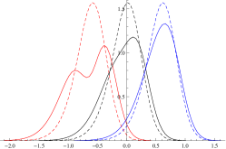
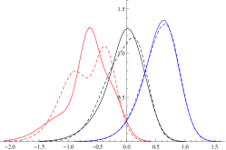
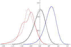
$n=4$	$n=5$	$n=6$
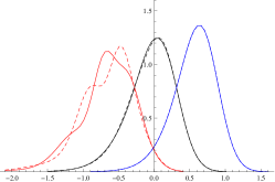
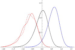
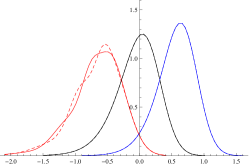
$n=7$	$n=7$	$n=9$

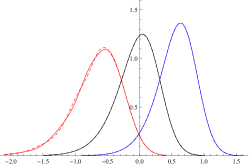
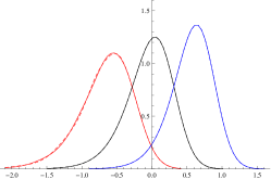
$$\nu_{i}(dz) =\frac{1}{\sqrt{2\pi s_{i}^{2}}}\exp\left(\frac{-(z-m_{i})^{2}}{2s_{i}^{2}}\right)dz$$ (122)

Figure 1: For different values of $n$ we plot as a function of $z$ the approximate transition densities $p^{(n)}(t,y,z)$ for $y=-0.6$ (solid red), $y=0.0$ (solid black) and $y=0.6$ (solid blue). In order to see the convergence, on each plot, we also graph $p^{(n-1)}(t,y,z)$ (dashed lines). Note that as $y$ moves closer to $-\infty$ (i) the transition densities become wider, (ii) convergence of the densities requires more terms and (iii) the densities have fatter tails on the left than on the right. All three phenomena are due to the fact that the local volatility and the jump-intensity rise as $y$ decreases to $-\infty$. The following parameters are used in these plots: $a_{0}=0.20$, $a_{1}=0.10$, $c_{0}=0.0$, $c_{1}=0.0$, $s_{0}=0.15$, $m_{0}=-0.10$, $s_{1}=0.15$, $m_{1}=-0.10$, $\varepsilon=1$, $\beta=-0.95$, $t=1.0$.

In Figure 1 we plot the approximate transition density $p^{(N)}$ for a CEV-like model with Gaussian jumps

$$\nu_{i}(dz) =\frac{1}{\sqrt{2\pi s_{i}^{2}}}\exp\left(\frac{-(z-m_{i})^{2}}{2s_{i}^{2}}\right)dz.$$ (92)

For the smallest initial value in the plot, $y=-0.6$ we see that $p^{(8)}$ and $p^{(9)}$ are virtually identical. As the initial value $y$ moves in the positive direction, fewer terms are required for convergence. For $y=0.0$, we see very little difference between $p^{(4)}$ and $p^{(5)}$. And for $y=0.6$, we see that $p^{(2)}$ and $p^{(3)}$ are nearly identical. This is not surprising, since the size of the perturbing term $\varepsilon e_{\beta}\mathscr{A}_{1}$ decreases as $y$ tends to infinity.

5.2.2 Comparison to Monte Carlo simulation

In order to test the accuracy of pricing formula (61) we compute the price of a series of call options with $N=10$. We once again assume Gaussian jumps, as in (92). For each call option, we also compute its price using Monte Carlo simulation. For the Monte Carlo simulations we use a standard Euler scheme with a time step of $10^{-3}$ years and run $10^{7}$ sample paths. As implied volatility – rather than price – is the more relevant quantity for call options, we convert prices to implied volatilities by inverting the Black-Scholes formula numerically (we examine our implied volatility expansion in the next section). In Figure 2 we plot the resulting implied volatilities as a function of the $\log$-moneyness to maturity ratio, $\text{LMMR}:=(k-y)/t$. For the strikes and maturities tested, we see very close agreement between the implied volatilities resulting from pricing approximation (61) and the implied volatilities resulting from the Monte Carlo simulation.

5.2.3 Implied Volatility Expansion

In section we examine the implied volatility expansion of Section 4. We continue to work in the CEV-like setting with $\eta=e_{\beta}$. But, we now set $\nu_{0}\equiv 0$ and $c_{0}=0$, which is an assumption of Section 4. We still assume $\nu_{1}$ is Gaussian, as in equation (92). We define the $\mathscr{O}(\varepsilon^{n})$ approximation of the implied volatility

$$\sigma^{(n)} :=\sum_{k=0}^{n}\varepsilon^{k}\sigma_{k},$$ (93)

where $\sigma_{0}=a_{0}$ and the $\{\sigma_{k}\}_{n=1}^{\infty}$ are given by (52). The values of $u_{n}$, which are needed for the implied volatility expansion, are computed using (60). In figure 3 we plot $\sigma^{(n)}$ for $n=0,1,\cdots,5$. In order to see how well the truncated implied volatility expansion approximates the exact implied volatility $\sigma^{\varepsilon}$ we also plot a proxy of $\sigma^{\varepsilon}$. Our proxy for $\sigma^{\varepsilon}$ is obtained by approximating $u^{\varepsilon}$ with $u^{(12)}$, and then by inverting the Black-Scholes formula numerically to obtain $\sigma^{\varepsilon}$. The price $u^{(12)}$ is computed using (61). Given the numerical results of Section 5.2.2, approximating $u^{\varepsilon}$ with $u^{(12)}$ should not introduce much error.

In Figure 3 we see very fast convergence of $\sigma^{(n)}$ to $\sigma^{\varepsilon}$ for $\text{LMMR}\in[-0.5,3.0]$. In this region $\sigma^{(3)}$ is nearly indistinguishable from $\sigma^{\varepsilon}$. Outside of this region, however, the implied volatility expansion does not converge. This is due to the fact that, for $\text{LMMR}\notin[-0.5,3.0]$ we have $|u^{\varepsilon}-u^{\mathrm{BS}}(a_{0})|>R$, where $R=R(t,y,k,a_{0})$ is the radius of convergence of the infinite series (42) with $\sigma_{0}=a_{0}$.

5.2.4 Calibration to S&P500 options

In order to demonstrate the applicability of the CEV-like models from Section 5 we perform a sample calibration to S&P500 options. For the calibration, we assume that jumps are Gaussian, i.e. that

$$\nu_{i}(dz)=\frac{\Gamma_{i}}{\sqrt{2\pi s^{2}}}\exp\left(\frac{(y-m)^{2}}{2s^{2}}\right)dz,$$

for $i=1,2$. We have assumed here a common mean $m$ and variance $s^{2}$, but have allowed for separate jump intensities $\Gamma_{0},\Gamma_{1}>0$. Thus the jump distribution remains constant, but the intensity $\Gamma_{0}+\varepsilon e^{\beta y}\Gamma_{1}$ varies with $y$. One could allow for additional flexibility by considering separate means and variances.

Let $\Phi$ be the set of model parameters and let $\Theta$ be the feasible set for these parameters. We denote by $\text{IV}(t,k;\Phi)$ the implied volatility of an option with time to maturity $t$ and $\log$-strike $k$, as computed using $\Phi$, and we denote by $\text{IV}^{obs}(t,k)$, the observed implied volatility of an option with time-to-maturity $t$ and $\log$-strike $k$. We formulate the calibration problem as a least-squares fit to the observed implied volatility. That is, we seek $\Phi^{*}$ such that

$$\inf_{\Phi\in\Theta}\sum_{{(t,k)\in(\mathcal{T},\mathcal{K})}}\left(\text{IV}^{obs}(t,k)-\text{IV}(t,k;\Phi)\right)^{2} =\sum_{{(t,k)\in(\mathcal{T},\mathcal{K})}}\left(\text{IV}^{obs}(t,k)-\text{IV}(t,k;\Phi^{*})\right)^{2},$$ (94)

where $(\mathcal{T},\mathcal{K})$ represents the set of all (maturity, strike) observed implied volatility data. Observe that we fit all maturities in the data set simultaneously; we do not fit maturity-by-maturity. Note, because $\nu_{0}\neq 0$ and $c_{0}\neq 0$, we are not in the setting of Section 4. Thus we must compute implied volatilities by first computing option prices using (61), and then by inverting the Black-Scholes formula numerically. The results of the calibration procedure are plotted in Figure 4. The figure clearly shows that the CEV-like model considered in this section provides a tight fit to implied volatility across maturities.

Using the parameters obtained in the calibration procedure, we run a series of numerical tests in order to investigate the computational cost of computing $\text{IV}^{(N)}$ (the implied volatility induced by $u^{(N)}$) for different values of $N$. As a point of comparison, we note that $u^{(0)}$ corresponds to the price of an option as computed in an exponential Lévy setting (i.e., an exponential Lévy model with no local-dependence). As demonstrated in Table 1, for $N=3$ we obtain we obtain implied volatilities that are accurate to two decimal places. These implied volatilities require roughly $2.22$ times as long to compute as the corresponding implied volatilities in an exponential Lévy setting.

5.2.5 Implied volatility asymptotics for CEV-like models with no jumps

In our last numerical experiment, we implement the implied volatility expansion outlined in Section 5.1. Under Assumption (25) we compute approximate implied volatilities $\sigma^{(2,M)}$ using (80) and (85). For comparison, we also plot the exact implied volatility $\sigma^{\varepsilon}$. To compute $\sigma^{\varepsilon}$, we first compute $u^{\varepsilon}$ using (61) and then we invert the Black-Scholes formula numerically. The results are plotted in Figure 5. With a time-to-maturity of $t=1/2$, we observe a nearly exact match between $\sigma^{(2,M)}$ and $\sigma^{\varepsilon}$ for $\log$-moneyness $k-y>-0.5$.

6 Conclusion

In this paper we introduce a class of Lévy-type models in which the diffusion coefficient, the Lévy measure and the default intensity all depend locally on the value of the underlying. Within this framework, we obtain a formula (written as an infinite series) for the price of a European option. Furthermore, we provide conditions under which this infinite series is guaranteed to converge. Additionally, we obtain an explicit expression for the implied volatility smile induced by a certain sub-class of Lévy-type models. This series is exact within its radius of convergence. As an example of our framework, we introduce a CEV-like Lévy-type model, which corrects some short-comings of the CEV model; namely (i) our choice of local volatility function does not drop to zero as the value of the underlying increases and (ii) our model permits the underlying asset to experience jumps. In this CEV-like setting, we show that option prices can be computed with the same level of efficiency as other models in which option prices are computed as Fourier-type integrals and we show that approximate implied volatilities can be computed explicitly without integration. We also test the accuracy of the pricing and implied volatility formulas in the CEV-like setting through numerical examples. And we show that one specific CEV-like model with normal jumps provides a tight fit to the observed S&P500 implied volatility surface.

Thanks

The authors would like to thank Bjorn Birnir, Stephan Sturm and two anonymous referees for their helpful comments.

Appendix A Proof of Proposition 3

We begin the proof by Fourier transforming the left-hand side of (26) and (27). We have

$$\langle\psi_{\lambda},(-\partial_{t}+\mathscr{A}_{0})u_{n}\rangle =-\partial_{t}\langle\psi_{\lambda},u_{n}\rangle+\langle\psi_{\lambda},\mathscr{A}_{0}u_{n}\rangle=-\partial_{t}\langle\psi_{\lambda},u_{n}\rangle+\langle\mathscr{A}^{*}_{0}\psi_{\lambda},u_{n}\rangle=(-\partial_{t}+\phi_{\lambda})\langle\psi_{\lambda},u_{n}\rangle,$$ (95)

where we use $\mathscr{A}^{*}_{0}\overline{\psi_{\lambda}}=\phi_{\lambda}\overline{\psi_{\lambda}}$. Fourier transforming the right-hand side of (27) and the initial conditions yields the following ODEs in the variable $t$ for $\langle\psi_{\lambda},u_{0}\rangle$ and for the sequence $(\langle\psi_{\lambda},u_{n}\rangle)_{n\geq 1}$:

$$\mathscr{O}(1): (-\partial_{t}+\phi_{\lambda})\langle\psi_{\lambda},u_{0}\rangle =0, \langle\psi_{\lambda},u_{0}(0,\cdot)\rangle =\langle\psi_{\lambda},h\rangle,$$ (96)

$$\mathscr{O}(\varepsilon^{n}): (-\partial_{t}+\phi_{\lambda})\langle\psi_{\lambda},u_{n}\rangle =-\langle\psi_{\lambda},\eta\mathscr{A}_{1}u_{n-1}\rangle, \langle\psi_{\lambda},u_{n}(0,\cdot)\rangle =0,\qquad n\geq 1.$$ (97)

The following solutions can easily be checked (e.g., by substitution)

$$\mathscr{O}(1): \langle\psi_{\lambda},u_{0}(t,\cdot)\rangle =e^{t\phi_{\lambda}}\langle\psi_{\lambda},h\rangle,$$ (98)

$$\mathscr{O}(\varepsilon^{n}): \langle\psi_{\lambda},u_{n}(t,\cdot)\rangle =\int_{0}^{t}dse^{(t-s)\phi_{\lambda}}\langle\psi_{\lambda},\eta\mathscr{A}_{1}u_{n-1}(s,\cdot)\rangle,\qquad n\geq 1.$$ (99)

Next, using (34), we obtain

$$\mathscr{O}(1): u_{0}(t,y) =\int_{\mathbb{R}}d\lambda e^{t\phi_{\lambda}}\langle\psi_{\lambda},h\rangle\psi_{\lambda}(y),$$ (100)

$$\mathscr{O}(\varepsilon^{n}): u_{n}(t,y) =\int_{\mathbb{R}}d\lambda\int_{0}^{t}dse^{(t-s)\phi_{\lambda}}\langle\psi_{\lambda},\eta\mathscr{A}_{1}u_{n-1}(s,\cdot)\rangle\psi_{\lambda}(y),\qquad n\geq 1.$$ (101)

Note that the sequence $(u_{n})_{n\geq 1}$ can be computed recursively. For example,

$$u_{1}(t,y) =\int_{\mathbb{R}}d\lambda\int_{0}^{t}dse^{(t-s)\phi_{\lambda}}\langle\psi_{\lambda},\eta\mathscr{A}_{1}u_{0}(s,\cdot)\rangle\psi_{\lambda}(y)$$ (102)

$$=\int_{\mathbb{R}}\int_{\mathbb{R}}d\lambda d\mu\int_{0}^{t}dse^{(t-s)\phi_{\lambda}}\langle\psi_{\lambda},\eta\mathscr{A}_{1}e^{s\phi_{\mu}}\langle\psi_{\mu},h\rangle\psi_{\mu}\rangle\psi_{\lambda}(y)$$ (103)

$$=\int_{\mathbb{R}}\int_{\mathbb{R}}d\lambda d\mu\int_{0}^{t}dse^{t\phi_{\lambda}+s(\phi_{\mu}-\phi_{\lambda})}\chi_{\mu}\langle\psi_{\lambda},\eta\psi_{\mu}\rangle\langle\psi_{\mu},h\rangle\psi_{\lambda}(y)$$ (104)

$$=\int_{\mathbb{R}}\int_{\mathbb{R}}d\lambda d\mu\left(\frac{e^{t\phi_{\mu}}-e^{t\phi_{\lambda}}}{\phi_{\mu}-\phi_{\lambda}}\right)\chi_{\mu}\langle\psi_{\lambda},\eta\psi_{\mu}\rangle\langle\psi_{\mu},h\rangle\psi_{\lambda}(y)$$ (105)

Generalizing the above recursion relation to arbitrary $n$, one finds expression (35) for $u_{n}$.

Appendix B Proof of Theorem 4

In this section, we will show that $u^{\varepsilon}$, given by (25) and (35), is a classical solution of the Cauchy problem (21) under the conditions of Theorem 4. Throughout this section, we define a Hilbert space $\mathscr{H}=L^{2}(\mathbb{R})$ with norm $\left\|{\cdot}\right\|=\langle\cdot,\cdot\rangle$ given by (28). Our strategy is to show that the closure of $\mathscr{A}^{\varepsilon}=\mathscr{A}_{0}+\varepsilon\eta\mathscr{A}_{1}$ (with a domain restricted to $\mathscr{H}$) generates a $C_{0}$-contraction semigroup $\mathscr{P}^{\varepsilon}=\{\mathscr{P}_{t}^{\varepsilon},t\geq 0\}$ in $\mathscr{H}$. The semigroup $\mathscr{P}^{\varepsilon}$ has the property that if $h\in{\rm dom}(\mathscr{A}^{\varepsilon})$ then $\mathscr{P}_{t}^{\varepsilon}h\in{\rm dom}(\mathscr{A}^{\varepsilon})$ (Engel and Nagel (2006), Proposition II.6.2) and $\left(-\partial_{t}+\mathscr{A}^{\varepsilon}\right)\mathscr{P}_{t}^{\varepsilon}h=0$ with initial condition $\mathscr{P}_{0}^{\varepsilon}h=h$. Thus, if we can show that $\mathscr{A}^{\varepsilon}$ generates a semigroup $\mathscr{P}^{\varepsilon}$, we can identify $u^{\varepsilon}(t,y)\equiv\mathscr{P}^{\varepsilon}h(t,y)$ as the unique classical solution to (21). Moreover, if it exists, the semigroup $\mathscr{P}_{t}^{\varepsilon}$ is given by $\mathscr{P}_{t}^{\varepsilon}=\exp(t\mathscr{A}^{\varepsilon})=\exp(t[\mathscr{A}_{0}+\varepsilon\eta\mathscr{A}_{1}])$, where the exponential is defined by

$$\exp(t\mathscr{A}^{\varepsilon}) :=\lim_{n\to\infty}\left(1-\frac{t}{n}\mathscr{A}^{\varepsilon}\right)^{-n},$$ (106)

and the solution $u^{\varepsilon}(t,y)=\mathscr{P}^{\varepsilon}h(t,y)$ inherits the analyticity of the exponential in the perturbing parameter $\varepsilon$. Thus, if $\mathscr{A}^{\varepsilon}$ generates a semigroup $\mathscr{P}^{\varepsilon}$, then $u^{\varepsilon}$ is an analytic function of $\varepsilon$, and has the representation (25).

We start by defining the domains of the operators $\mathscr{A}_{0}$, $\mathscr{A}_{1}$ and $\eta\mathscr{A}_{1}$: ${\rm dom}(\mathscr{A}_{i}):=\{u\in\mathscr{H}:\left\|{\mathscr{A}_{i}u}\right\|<\infty\}$ for $i=0,1$ and ${\rm dom}(\eta\mathscr{A}_{1}):=\{u\in\mathscr{H}:\left\|{\eta\mathscr{A}_{1}u}\right\|<\infty\}$. Note that

$$\left\|\mathscr{A}_{0}u\right\|^{2} =\int_{\mathbb{R}}d\lambda|\langle\psi_{\lambda},u\rangle|^{2}|\phi_{\lambda}|^{2}, \left\|\mathscr{A}_{1}u\right\|^{2} =\int_{\mathbb{R}}d\lambda|\langle\psi_{\lambda},u\rangle|^{2}|\chi_{\lambda}|^{2}, \left\|\eta\right\|^{2} =\int_{\mathbb{R}}d\lambda|\langle\psi_{\lambda},\eta\rangle|^{2}.$$ (107)

Thus by (36), we have ${\rm dom}(\mathscr{A}_{0})\subseteq{\rm dom}(\mathscr{A}_{1})$. Since $\eta\in\mathscr{S}$, then $\left\|{\eta\mathscr{A}_{1}u}\right\|^{2}\leq\left\|{\eta}\right\|^{2}\cdot\left\|{\mathscr{A}_{1}u}\right\|^{2}$ is finite for any $u\in{\rm dom}(\mathscr{A}_{1})$. Therefore the inclusions $\mathscr{S}\subseteq{\rm dom}(\mathscr{A}_{0})\subseteq{\rm dom}(\mathscr{A}_{1})\subseteq{\rm dom}(\eta\mathscr{A}_{1})$ hold. Therefore since $\mathscr{S}$ is a dense subset of $\mathscr{H}$ (see Jacob (2001), Corollary 2.6.1), the operators $\mathscr{A}_{0}$, $\mathscr{A}_{1}$ and $\eta\mathscr{A}_{1}$ are densely defined in $\mathscr{H}$. To show that $\mathscr{A}^{\varepsilon}$ generates a semigroup $\mathscr{P}^{\varepsilon}$ we recall the following theorem from Chernoff (1972):

Theorem 27.

Let $\mathscr{A}$ be the generator of a $C_{0}$-contraction semigroup $\mathscr{P}_{t}^{0}\equiv\exp(t\mathscr{A})$ on a Banach space, and $\varepsilon\mathscr{B}$ a dissipative operator with a densely defined adjoint. If there exist two real constants $A\geq 0$ and $B\leq 1$ such that the inequality $\left\|{\varepsilon\mathscr{B}u}\right\|\leq A\left\|{u}\right\|+B\left\|{\mathscr{A}u}\right\|$ holds for all $u\in{\rm dom}(\mathscr{A})$ (i.e., the operator $\varepsilon\mathscr{B}$ is bounded relative to $\mathscr{A}$ with relative bound $B$), then the closure of $\mathscr{A}^{\varepsilon}:=\mathscr{A}+\varepsilon\mathscr{B}$ generates a $C_{0}$-contraction semigroup $\mathscr{P}_{t}^{\varepsilon}=\exp(t\mathscr{A}^{\varepsilon})$.

We now check the conditions of Theorem 27 with $\mathscr{A}_{0}\equiv\mathscr{A}$ and $\varepsilon\eta\mathscr{A}_{1}\equiv\varepsilon\mathscr{B}$. First, by Corollary II.3.17 in Engel and Nagel (2006), $\mathscr{A}_{0}$, as the generator of a Lévy process that is an exponentially special semimartingale, generates a $C_{0}$-contraction semigroup. Next, by Theorem 2.12 in Hoh (1998), $\varepsilon\eta\mathscr{A}_{1}$ satisfies the positive maximum principle, and hence is dissipative (Ethier and Kurtz (1986), Lemma 4.2.1). Since $\eta\in\mathscr{S}$ and since Hilbert spaces are reflexive, then $\varepsilon\eta\mathscr{A}_{1}$ has a densely defined adjoint (see the discussion after the main theorem in Chernoff (1972)). Theorem 4 will then follow if we can prove that $\varepsilon\eta\mathscr{A}_{1}$ is bounded relative to $\mathscr{A}_{0}$ with relative bound $B$.

Proposition 28.

Suppose that there exist two constants $A\geq 0$ and $B\leq 1$ such that $\varepsilon$ satisfies

$$\varepsilon^{2} \leq\inf_{\lambda\in\mathbb{R}}\frac{A^{2}+B^{2}|\phi_{\lambda}|^{2}}{\left\|\eta\right\|^{2}\cdot|\chi_{\lambda}|^{2}}.$$ (108)

Then $\varepsilon\eta\mathscr{A}_{1}$ is bounded relative to $\mathscr{A}_{0}$ with relative bound $B$.

Proof.

For any $u\in{\rm dom}(\mathscr{A}_{0})$, the inequality in the proposition holds if and only if $\varepsilon^{2}\leq\frac{A^{2}+B^{2}|\phi_{\lambda}|^{2}}{\left\|\eta\right\|^{2}\cdot|\chi_{\lambda}|^{2}}$ holds for all $\lambda\in\mathbb{R}$. This in turn is equivalent to $0\leq A^{2}+B^{2}|\phi_{\lambda}|^{2}-\varepsilon^{2}\left\|\eta\right\|^{2}\cdot|\chi_{\lambda}|^{2}$ for any $\lambda\in\mathbb{R}$, which implies that

$$0\leq\int_{\mathbb{R}}d\lambda|\langle\psi_{\lambda},u\rangle|^{2}\left(A^{2}+B^{2}|\phi_{\lambda}|^{2}-\varepsilon^{2}\left\|\eta\right\|^{2}\cdot|\chi_{\lambda}|^{2}\right)=A^{2}\left\|u\right\|^{2}+B^{2}\left\|\mathscr{A}_{0}u\right\|^{2}-\varepsilon^{2}\left\|\eta\right\|^{2}\cdot\left\|\mathscr{A}_{1}u\right\|^{2}.$$

This then implies $\left\|\varepsilon\eta\mathscr{A}_{1}u\right\|^{2}\leq A^{2}\left\|u\right\|^{2}+B^{2}\left\|\mathscr{A}_{0}u\right\|^{2}$. Since $\left\|\eta\mathscr{A}_{1}u\right\|\leq\left\|\eta\right\|\cdot\left\|\mathscr{A}_{1}u\right\|$, we then deduce the final inequality $\left\|\varepsilon\eta\mathscr{A}_{1}u\right\|\leq A\left\|u\right\|+B\left\|\mathscr{A}_{0}u\right\|$, and the proposition follows. ∎

We have now shown that $\mathscr{A}^{\varepsilon}$ generates a semigroup $\mathscr{P}^{\varepsilon}$. Therefore, we identify $u^{\varepsilon}(t,y)=\mathscr{P}_{t}^{\varepsilon}h(y)$ and we note that $u^{\varepsilon}(t,y)$ is analytic in the perturbing parameter $\varepsilon$.

Appendix C Mathematica code for computing $\sigma^{(2,M)}$

The following code will produce $\sigma^{(2,M)}$ from equation (85) with $M=10$.

$$M =10;$$ (109)

$$\phi[\lambda\_] =\frac{1}{2}\text{a0}^{2}\left(-\lambda^{2}-i\lambda\right);$$ (110)

$$\chi[\lambda\_] =\frac{1}{2}\text{a1}^{2}\left(-\lambda^{2}-i\lambda\right);$$ (111)

$$\text{b1}[\text{t$\_$},\text{a0$\_$},\text{a1$\_$}] =\text{CoefficientList}\left[\sum_{n=1}^{M}\frac{t{}^{\wedge}n}{n!}(\phi[-id-i\beta]-\phi[-id]){}^{\wedge}(n-1)\frac{1}{2}\text{a1}^{2},d\right];$$ (112)

$$\text{b2}[\text{t$\_$},\text{a0$\_$},\text{a1$\_$}] =\text{CoefficientList}\Big{[}\sum_{n=2}^{M}\frac{t{}^{\wedge}n}{n!}\sum_{k=1}^{n-1}\text{Binomial}[n-1,k](-\phi[-id]){}^{\wedge}(n-1-k)$$ (113)

$$\qquad\sum_{m=0}^{k-1}(\phi[-id-i\beta]){}^{\wedge}m(\phi[-id-2i\beta]){}^{\wedge}(k-1-m)\chi[-id-i\beta]\frac{1}{2}\text{a1}^{2},d\Big{]};$$ (114)

$$\text{dp}[\text{t$\_$},\text{y$\_$},\text{a0$\_$},\text{k$\_$}] =(y-k+(\text{a0}{}^{\wedge}2/2)t)/(\text{a0}\sqrt{t});$$ (115)

$$\text{$\sigma$1}[\text{t$\_$},\text{y$\_$},\text{a0$\_$},\text{a1$\_$},\beta\_,\text{k$\_$}] =\text{Exp}[\beta y]\sum_{n=0}^{M-1}\text{b1}[t,\text{a0},\text{a1}][[n+1]]$$ (116)

$$\qquad\text{FullSimplify}\left[\frac{D[\text{Exp}[y-\text{dp}[t,y,\text{a0},k]{}^{\wedge}2/2],\{y,n\}]}{t\,\text{a0}\,\text{Exp}[y-\text{dp}[t,y,\text{a0},k]{}^{\wedge}2/2]}\right];$$ (117)

$$\text{$\sigma$1}[\text{t$\_$},\text{y$\_$},\text{a0$\_$},\text{a1$\_$},\beta\_,\text{k$\_$}] =\text{Exp}[2\beta y]\sum_{n=0}^{M-1}\text{b2}[t,\text{a0},\text{a1}][[n+1]]$$ (118)

$$\qquad\text{FullSimplify}\left[\frac{D[\text{Exp}[y-\text{dp}[t,y,\text{a0},k]{}^{\wedge}2/2],\{y,n\}]}{t\,\text{a0}\,\text{Exp}[y-\text{dp}[t,y,\text{a0},k]{}^{\wedge}2/2]}\right]$$ (119)

$$\qquad-\frac{1}{2}\Big{(}\text{$\sigma$1}[t,y,\text{a0},\text{a1},\beta,k]\Big{)}{}^{\wedge}2\left(\frac{(k-y){}^{\wedge}2}{t\text{a0}{}^{\wedge}3}-\frac{t\,\text{a0}}{4}\right);$$ (120)

$$\sigma{2M}[\text{t$\_$},\text{y$\_$},\text{a0$\_$},\text{a1$\_$},\beta\_,\varepsilon\_,\text{k$\_$}] =\text{a0}+\varepsilon\,\text{$\sigma$1}[t,y,\text{a0},\text{a1},\beta,k]+\varepsilon{}^{\wedge}2\,\text{$\sigma$2}[t,y,\text{a0},\text{a1},\beta,k];$$ (121)

$t=0.125$	$t=0.25$
$t=0.5$	$t=1.0$

$$\nu_{i}(dz) =\frac{1}{\sqrt{2\pi s_{i}^{2}}}\exp\left(\frac{-(z-m_{i})^{2}}{2s_{i}^{2}}\right)dz$$ (123)

Figure 2: In the above plots, we compute option prices using formula (61) with $N=10$ and also by Monte Carlo simulation. We then convert these prices to implied volatilities by inverting Black-Scholes numerically. We do not use the implied volatility expansion described in Section 4. The solid line corresponds to implied volatilities computed using pricing formula (61). The circles correspond to implied volatilities resulting from the Monte Carlo simulation. Units on the horizontal axis are logmoneyness to maturity ratios ($\text{LMMR}:=(k-y)/t$). Note the steep skew, which is due to the fact that the local volatility and the jump intensity increase as the value of the underlying drops. The following parameters are used in this plot: $a_{0}=0.20$, $a_{1}=0.10$, $c_{0}=0.00$, $c_{1}=0.00$, $s_{0}=0.20$, $s_{1}=0.10$, $m_{0}=-0.20$, $m_{1}=-0.10$, $\varepsilon=1.0$, $\beta=-1.25$, $y=-0.10$.

$n=0$	$n=1$
$n=2$	$n=3$
$n=4$	$n=5$

$$\nu_{0}(dz) =0, \nu_{1}(dz) =\frac{1}{\sqrt{2\pi s_{1}^{2}}}\exp\left(\frac{-(z-m_{1})^{2}}{2s_{i}^{2}}\right)dz.$$ (124)

Figure 3: We plot $\sigma^{(n)}$, the order $\mathscr{O}(\varepsilon^{n})$ approximation of implied volatility (solid black), and $\sigma^{\varepsilon}$, the exact implied volatility (dashed black) as a function of LMMR. The following parameters are used in these plots: $a_{0}=0.30$, $a_{1}=0.00$, $c_{0}=0.00$, $c_{1}=0.00$, $s_{1}=0.2$, $m_{1}=-0.40$, $\varepsilon=4$, $\beta=-1.25$, $t=0.125$, $y=0.10$.

87 DTM	115 DTM	142 DTM

Figure 4: Using the CEV-like model from Section 5, we perform a calibration to S&P500 options from January 24, 2012. The horizontal axis is in units of $\log$-moneyness: $\text{LM}:=k-y$ and the vertical axis in units of implied volatility. The fit is a least-squares algorithm to implied volatilities across the three maturities. We emphasize that we do not fit maturity-by-maturity. The Lévy measures $\nu_{0}$ and $\nu_{1}$ are Gaussian with common mean $m$ and variance $s$ but different intensities $\Gamma_{0}$ and $\Gamma_{1}$. Thus, we allow the jump intensity, but not the jump distribution, to change as a function of $y$. The parameters resulting from the calibration are as follows: $a_{0}=0.059$, $c_{0}=0.009$, $\Gamma_{0}=1.105$, $a_{1}=0.057$, $c_{1}=0.010$, $\Gamma_{1}=1.095$, $m=-0.076$, $s=0.078$, $\beta=0.410$, $\varepsilon=1.00$. Without loss of generality, we assume $y=0$, which simply results in a rescaling of parameters.

$N$	$T_{N}/T_{0}$					$\text{IV}^{(N)}$
0	1.00	0.2420	0.2162	0.1933	0.1719	0.1486	0.1222	0.1014	0.0929	0.0963	0.1046
1	1.04	0.2929	0.2683	0.2476	0.2306	0.2166	0.2006	0.1676	0.1318	0.1183	0.1211
2	1.49	0.2960	0.2709	0.2479	0.2265	0.2049	0.1841	0.1743	0.1558	0.1341	0.1307
3	2.22	0.2951	0.2698	0.2475	0.2276	0.2088	0.1887	0.1634	0.1547	0.1429	0.1354
4	3.26	0.2953	0.2701	0.2475	0.2272	0.2077	0.1877	0.1694	0.1483	0.1437	0.1379
5	4.48	0.2952	0.2700	0.2475	0.2273	0.2079	0.1879	0.1674	0.1518	0.1404	0.1390
6	6.16	0.2952	0.2700	0.2475	0.2273	0.2080	0.1878	0.1675	0.1519	0.1403	0.1391
	LM	-0.225	-0.180	-0.135	-0.090	-0.045	0.000	0.045	0.090	0.135	0.180

Table 1: Using the parameters obtained in the calibration to S&P500 options (see Figure 4) we compute approximate prices $u^{(N)}$ using equation (61). We then compute implied volatilities ($\text{IV}^{(N)}$) by inverting the Black-Scholes pricing formula numerically. We denote by $T_{N}$ the computational time required to compute implied volatilities for a series of strikes (listed above in unites of $\log$-moneyness: $\text{LM}:=k-y$) with a time to maturity of 142 days. Note that $T_{0}$ corresponds to the time it takes to compute IV’s for an exponential Lévy model.

Figure 5: We consider here the model proposed in Section 5.1. We plot the exact implied volatility $\sigma^{\varepsilon}$ (solid), as well as the approximations $\sigma^{(2,M)}$ (dashed) and $\sigma^{(1,M)}$ (dotted) as a function of $\log$-moneyness: $\text{LM}:=k-y$. In the above plot we use the following parameters: $t=0.5$, $y=0.0$, $\beta=-2.0$, $\varepsilon=1.0$, $a_{0}=0.5$ and $a_{1}=0.3$. Observe that $\sigma^{(2,M)}$ closely approximates $\sigma^{\varepsilon}$ for all $\text{LM}>-0.5$.

References

• Abramowitz and Stegun (1964) Abramowitz, M. and I. Stegun (1964). Handbook of mathematical functions with formulas, graphs, and mathematical tables, Volume 55. Dover publications.
• Benhamou et al. (2009) Benhamou, E., E. Gobet, and M. Miri (2009). Smart expansion and fast calibration for jump diffusions. Finance and Stochastics 13(4), 563–589.
• Bensoussan and Lions (1984) Bensoussan, A. and J. Lions (1984). Impulse control and quasi-variational inequalities. Bordas Editions.
• Boyarchenko and Levendorskii (2002) Boyarchenko, S. and S. Levendorskii (2002). Non-Gaussian Merton-Black-Scholes Theory. World Scientific.
• Brown and Churchill (1996) Brown, J. and R. Churchill (1996). Complex variables and applications, Volume 7. McGraw-Hill New York, NY.
• Carr and Linetsky (2006) Carr, P. and V. Linetsky (2006). A jump to default extended CEV model: An application of bessel processes. Finance and Stochastics 10(3), 303–330.
• Chernoff (1972) Chernoff, P. R. (1972). Perturbations of dissipative operators with relative bound one. Proceedings of the American Mathematical Society 33(1).
• Christoffersen et al. (2009) Christoffersen, P., K. Jacobs, and Ornthanalai (2009). Exploring Time-Varying Jump Intensities: Evidence from S&P500 Returns and Options. CIRANO.
• Cont and Tankov (2004) Cont, R. and P. Tankov (2004). Financial modelling with jump processes, Volume 2. Chapman & Hall.
• Cox (1975) Cox, J. (1975). Notes on option pricing I: Constant elasticity of diffusions. Unpublished draft, Stanford University. A revised version of the paper was published by the Journal of Portfolio Management in 1996.
• Deuschel et al. (2013) Deuschel, J., P. Friz, A. Jacquier, and S. Violante (2013). Marginal density expansions for diffusions and stochastic volatility, part i: Theoretical foundations. Forthcoming in Communications on Pure and Applied Mathematics.
• Dirac (1927) Dirac, P. A. M. (1927). The physical interpretation of the quantum dynamics. Proceedings of the Royal Society of London. Series A, Containing Papers of a Mathematical and Physical Character 113(765), pp. 621–641.
• Engel and Nagel (2006) Engel, K. and R. Nagel (2006). A short course on operator semigroups. Springer.
• Eraker (2004) Eraker, B. (2004). Do stock prices and volatility jump? reconciling evidence from spot and option prices. The Journal of Finance 59(3), 1367–1404.
• Ethier and Kurtz (1986) Ethier, S. and T. Kurtz (1986). Markov processes: characterization and convergence, Volume 6. Wiley New York.
• Fouque et al. (2011) Fouque, J.-P., G. Papanicolaou, R. Sircar, and K. Solna (2011). Multiscale Stochastic Volatility for Equity, Interest-Rate and Credit Derivatives. Cambridge University Press.
• Hoh (1998) Hoh, W. (1998). Pseudo differential operators generating markov processes. Habilitations-schrift, Universität Bielefeld.
• Jacob (2001) Jacob, N. (2001). Pseudo differential operators and markov processes. vol. 1: Fourier analysis and semigroups.
• Jacod and Shiryaev (1987) Jacod, J. and A. N. Shiryaev (1987). Limit theorems for stochastic processes, Volume 288. Springer-Verlag Berlin.
• Lewis (2001) Lewis, A. (2001). A simple option formula for general jump-diffusion and other exponential Lévy processes.
• Linetsky (2007) Linetsky, V. (2007). Chapter 6 spectral methods in derivatives pricing. In J. R. Birge and V. Linetsky (Eds.), Financial Engineering, Volume 15 of Handbooks in Operations Research and Management Science, pp.  223 – 299. Elsevier.
• Lipton (2002a) Lipton, A. (2002a). Mathematical methods for foreign exchange. World Scientific.
• Lipton (2002b) Lipton, A. (2002b). The vol smile problem. Risk (February), 61–65.
• Lorig et al. (2013) Lorig, M., S. Pagliarani, and A. Pascucci (2013). A family of density expansions for lévy-type processes with default. ArXiv preprint arXiv:1304.1849.
• Mendoza-Arriaga et al. (2010) Mendoza-Arriaga, R., P. Carr, and V. Linetsky (2010). Time-changed markov processes in unified credit-equity modeling. Mathematical Finance 20, 527–569.
• Øksendal and Sulem (2005) Øksendal, B. and A. Sulem (2005). Applied stochastic control of jump diffusions. Springer Verlag.
• Pagliarani et al. (2011) Pagliarani, S., A. Pascucci, and R. Candia (2011). Adjoint expansions in local Lévy models.