Onsager Relations in Coupled Electric, Thermoelectric and Spin Transport:
The Ten-Fold Way

Abstract

Hamiltonian systems can be classified into ten classes, in terms of the presence or absence of time-reversal symmetry, particle-hole symmetry and sublattice/chiral symmetry. We construct a quantum coherent scattering theory of linear transport for coupled electric, heat and spin transport; including the effect of Andreev reflection from superconductors. We derive a complete list of the Onsager reciprocity relations between transport coefficients for coupled electric, spin, thermoelectric and spin caloritronic effects. We apply these to all ten symmetry classes, paying special attention to specific additional relations that follow from the combination of symmetries, beyond microreversibility. We discuss these relations in several illustrative situations. We show the reciprocity between spin-Hall and inverse spin-Hall effects, and the reciprocity between spin-injection and magnetoelectric spin currents. We discuss the symmetry and reciprocity relations of Seebeck, Peltier, spin-Seebeck and spin-Peltier effects in systems with and without coupling to superconductors.

I Introduction

Onsager’s reciprocity relations are cornerstones of nonequilibrium statistical mechanics Onsager1 ; Onsager2 . They relate linear response coefficients between flux densities and thermodynamic forces to one another. They are based on the fundamental principle of microreversibility which, for systems with time-reversal symmetry (TRS), says that “if the velocities of all the particles present are reversed simultaneously the particles will retrace their former paths, reversing the entire succession of configurations” Onsager1 . When TRS is broken, microreversibility further requires to invert all TRS breaking fields, which, to fix ideas, one may take as magnetic fields, fluxes or exchange fields. Combining all of them into a single multi-component field ${\cal H}$, the Onsager reciprocity relations read Onsager1 ; Onsager2

$${\cal L}_{ij}({\cal H})={\cal L}_{ji}(-{\cal H})\,,$$ (1)

where the linear coefficient ${\cal L}_{ij}$ determines the response of the flux density ${\cal J}_{i}$ – for instance the electric or heat current – to a weak thermodynamic force ${\cal X}_{j}$ – for instance an electric field or a temperature gradient. Thus the precise form of the Onsager reciprocity relations depends on the symmetries of the system. Seminal works have classified noninteracting quantum mechanical systems into ten general symmetry classes dys62 ; ver93 ; alt97 , and it is the purpose of the present manuscript to derive Onsager’s relations for all these symmetry classes. Four of them, in particular, combine two different types of quasiparticles alt97 , with microscopic representations including, e.g. hybrid systems where quantum coherent normal metallic conductors are connected to superconductors. Since at sub-gap energies an interface between a normal metal and a superconductor blocks heat currents but not electric currents  And64 , it is natural to ask whether the Onsager reciprocity relation between, say, the Seebeck and Peltier thermoelectric coefficients survives in such systems. Onsager relations in the presence of superconductivity have been discussed rather incompletely until now Cla96 ; Vir04 ; Tit08 ; Jac10 ; Eng11 , despite much experimental Eom98 ; Cad09 ; Par03 and theoretical Cla96 ; Vir04 ; Tit08 ; Jac10 ; Eng11 ; Sev00 ; Bez03 interest in thermoelectric transport properties of hybrid normal-metallic/superconducting systems.

Symmetry class		TRS	PHS	SLS	Physical example
Wigner-Dyson	A (unitary)	0	0	0	mag. flux . (no SC)
	AI (orthog.)	$+1$	0	0	no mag. flux & no spin-orbit . (no SC)
	AII (sympl.)	$-1$	0	0	spin-orbit & no mag. flux. (no SC)
Chiral	AIII (unitary)	0	0	1	mag. flux & bipartite lattice . (no SC)
	BDI (orthog.)	$+1$	+1	1	no mag. flux & no spin-orbit & bipartite lattice . (no SC)
	CII (sympl.)	$-1$	$-1$	1	spin-orbit & no mag. flux & bipartite lattice . (no SC)
Altland-Zirnbauer	D	0	$+1$	0	SC, mag. flux, & spin-orbit
	C	0	$-1$	0	SC, mag. flux, & no spin-orbit
	DIII	$-1$	$+1$	1	SC, no mag. flux, & spin-orbit
	CI	$+1$	$-1$	1	SC, no mag. flux, & no spin-orbit

Table 1: The ten-fold symmetry classification of Hamiltonians. The second column from the left refers to Cartan’s nomenclature for symmetric spaces alt97 , the three middle columns indicate whether the classes have broken (0) or unbroken ($\pm 1$) time-reversal symmetry (TRS), particle-hole symmetry (PHS) and sublattice symmetry (SLS), while the rightmost column mentions microscopic realizations in each class, with SC indicating the presence of superconductivity. Aside from the indicated bipartite lattice models with preserved sublattice symmetry, the chiral classes are also realized in low-energy models for quantum chromodynamics ver93 . Spin rotational symmetry (SRS) is present in classes AI, BDI, C and CI, absent in classes AII, CII, D and DIII, and irrelevant in classes A and AIII.

Further motivation is provided by fundamental aspects of spintronics Fab07 and spin caloritronics (spin-Seebeck and spin-Peltier effects) bau11 , where Onsager relations are of significant interest han05 ; sas07 ; tse08 ; bau10 ; Brataas1 ; Brataas2 . As a matter of fact, reciprocity relations decisively helped in experimentally uncovering elusive spin effects, by suggesting to measure electric effects that are reciprocal to them. As but one example, we mention the inverse spin Hall effect val06 ; Sai06 ; Kim07 ; Sek08 ; Liu11 , where a transverse electric current or voltage is generated by an injected spin current Gorini . Onsager relations also put constraints on the measurement of spin currents ada06 ; stano1 that can be circumvented in the nonlinear regime only vanwees ; stano2 . Accordingly, we will incorporate spin currents and accumulations into our formalism. Several of the Onsager relations for spin transport we derive below appeared in one way or another in earlier publications, see in particular Refs. [sas07, ; tse08, ; bau10, ; Brataas1, ; Brataas2, ; val06, ; ada06, ]. Here, we summarize them in a unified way and extend them to all ten symmetry classes. We are unaware of earlier discussions of Onsager relations for spin transport in the presence of superconductivity.

The classification into ten different symmetry classes has recently received renewed attention, because the existence of topologically nontrivial phases Qi11 depends on the system’s symmetries and its dimensionality sch08 . The Onsager relations we derive below depend only on fundamental symmetries and are equally valid in topologically trivial and nontrivial states caveat1 . In several instances, however, specific additional relations exist, that arise because of the conservation of each quasiparticle species (relevant to systems without superconductor so that there are no Andreev processes converting electrons into holes and vice-versa), the presence of particle-hole symmetry or sublattice/chiral symmetry. This is the case, for instance, for two-terminal thermoelectric transport in the Wigner-Dyson symmetry classes  dys62 , where the relation between Seebeck, $B$ and Peltier, $\Gamma$ coefficients reads equivalently $B({\cal H})T_{0}=\Gamma({\cal H})$ or $B({\cal H})T_{0}=\Gamma(-{\cal H})$, with the base temperature $T_{0}$, because of the additional reciprocity relation $\Gamma({\cal H})=\Gamma(-{\cal H})$ But90 . Below, we pay special attention to these nongeneric relations.

The manuscript is organized as follows. In Section II, we discuss the ten symmetry classes, and the crossover between Altland-Zirnbauer and the Wigner-Dyson classes as the temperature is raised in hybrid systems. In Section III we derive and list the symmetries that the ${\cal S}$-matrix satisfies in all classes. Onsager relations will follow from these symmetries, once they are inserted into scattering theory expressions for the linear transport coefficients. In Section IV, we formulate the problem in terms of the scattering matrix of the system and connect the Onsager coefficients to the system’s scattering matrix. In Section V we list the general reciprocity relations and mention additional ones occurring in special circumstances. Finally, in Sections VI and VII, we discuss some cases of importance and the associated Onsager relations in systems with coupled electric and spin transport, superconductors or chiral symmetries. Conclusions are given in Section VIII

Symmetry class		TRS	PHS	SLS	Physical example
Crossovers	D $\to$ A	0	$+1\to 0$	0	as D but $(\tau_{\rm Andr}k_{\rm B}T_{0})$ is not small
for Andreev	C $\to$ A	$0$	$-1\to 0$	0	as C but$(\tau_{\rm Andr}k_{\rm B}T_{0})$ is not small
interfero.	DIII $\to$ AII	$-1$	$+1\to 0$	1 $\to$ 0	as DIII but $(\tau_{\rm Andr}k_{\rm B}T_{0})$ is not small
	CI $\to$ AI	$+1$	$-1\to 0$	1$\to$ 0	as CI but $(\tau_{\rm Andr}k_{\rm B}T_{0})$ is not small

Table 2: Crossovers from the Altland-Zirnbauer to the Wigner-Dyson classes. Increasing the temperature breaks PHS so that the quasiparticle excitation energy $\epsilon$ cannot be treated as small. One way to break PHS is to make $(k_{\rm B}T_{0})\tau_{\rm Andr}$ not negligible, where $\tau_{\rm Andr}$ is a timescale associated with impinging on or returning to the superconducting contacts.

II The ten-fold way

Hamiltonian systems are classified according to the presence or absence of fundamental symmetries. The historical classification scheme dys62 ; alt97 is based on TRS and spin-rotational symmetry (SRS). Three Wigner-Dyson classes are defined in this way. Using the Cartan nomenclature for symmetric spaces, the class A has both symmetries broken, the class AI has both symmetries present, and the class AII has broken SRS but unbroken TRS. When TRS is broken, the presence or absence of SRS only affects the size of the Hamiltonian matrix — and not its symmetry — and there is thus no fourth class.

Chiral classes were next introduced ver93 , which capture the structure of the QCD Dirac operators. Beside relativistic fermions, they are also appropriate to describe bipartite lattice Hamiltonians with unbroken sublattice symmetry (SLS). Examples include two-dimensional square and hexagonal lattices, as well as three-dimensional cubic lattices without mass/on-site term, the latter generically breaking SLS. Here also, there are three classes, with (apart from their chiral symmetry) the same symmetries as the Wigner-Dyson classes.

Finally, four more classes of Bogoliubov-de Gennes (BdG) Hamiltonians appear - the Altland-Zirnbauer classes alt97 - when normal metals are brought into contact with superconductors: with SRS (C and CI) and without SRS (D and DIII), with TRS (CI and DIII) and without TRS (C and D). When dealing with such systems, we use a convention where the BdG Hamiltonian reads

$$H=\left(\begin{array}[]{cc}h-\mu_{\rm sc}&\Delta\\ \Delta^{*}&\mu_{\rm sc}-\sigma^{(y)}h^{*}\sigma^{(y)}\end{array}\right)\,,$$ (4)

with the Pauli matrix $\sigma^{(y)}$ acting on the spin degree of freedom and the chemical potential $\mu_{\rm sc}$ on the superconductor. With this convention, used for example in Refs. [Slevin1996, ; Oreg-Majorana-2010, ], the second-quantized Bogoliubov-de Gennes Hamiltonian is ${\textstyle{\frac{1}{2}}}\bm{c}^{\dagger}H\bm{c}$, where

$$\bm{c}^{\dagger}=(c_{e\uparrow}^{\dagger},c_{e\downarrow}^{\dagger},c_{h\downarrow}^{\dagger},-c_{h\uparrow}^{\dagger}).$$ (5)

with $c_{e\uparrow}^{\dagger}$ being the vector of creation operator for all $k$-states of spin-$\uparrow$ electrons, etc. This has the hole sector rotated by $i\sigma^{(y)}$ with respect to the Hamiltonian in Refs. [alt97, ; sch08, ]. The form of Eq. (4) has the advantage that upon assuming SRS (so $h^{*}$ commutes with $\sigma^{(y)}$), it immediately reduces to that used in Refs. [Cla96, ; deGennes-book, ; Tinkham-book, ; Beenakker-review, ].

Ref. [sch08, ] introduced a unifying ten-fold classification scheme for all the above Hamiltonians. They considered TRS and particle-hole symmetry (PHS), which can both be represented by antiunitary operators, and accordingly, these two symmetries can be either broken, or unbroken. In the former case, we represent this by a $0$, while in the latter case, the antiunitary operator squares to either $+1$ or $-1$. A squared TRS of $+1$ corresponds to spinless or integer-spin particles, while a squared TRS of $-1$ corresponds to half-integer-spin particles. A squared PHS of $+1$ corresponds to triplet pairing, while a squared PHS of $-1$ corresponds to singlet pairing in a Bogoliubov-de Gennes Hamiltonian footnote:TRS-plus-minus-one . Naively one would think that this leads to $3\times 3=9$ classes, however there are two distinct possibilities when both TRS and PHS are broken. In this case, the symmetry represented by the product of the two antiunitary operators gives either $0$ (when the corresponding symmetry is broken) or $+1$. This finally gives $3\times 3-1+2=10$ symmetry classes again. Using the just defined three indices, we summarize the ten symmetry classes in Table 1, where we additionally mention relevant physical realizations for each of them.

In this classification, the possible symmetries that the Hamiltonian $H$ satisfies are (i) TRS : $H=THT^{-1}$, with $T=-iK$, with the complex conjugation operator $K$ in the spinless case, and $T=-i\sigma^{(y)}K$ for spin-$1/2$ fermions, with the Pauli matrix $\sigma^{(y)}$ acting in spin space; (ii) PHS : $H=-PHP^{-1}$, with $P=-i\sigma^{(y)}\tau^{(y)}K$, with the Pauli matrix $\tau^{(y)}$ acting in Nambu space caveat2 ; (iii) SLS : $H=-\eta^{(z)}H\eta^{(z)}$, with the Pauli matrix $\eta^{(z)}$ acting on sublattice space (bipartite lattices are assumed here).

TRS, SRS and SLS can be broken by an orbital magnetic field, spin-orbit interaction and mass/on-site terms respectively. The Altland-Zirnbauer classes assume PHS, which strictly speaking forces thermoelectric effects to vanish identically. PHS can be broken, for instance, by moving away in energy from the special $\epsilon=0$ symmetry point – the superconductor’s chemical potential. This occurs upon increasing the temperature, when the latter exceeds a Thouless energy scale, $E_{\rm T}\simeq\tau^{-1}_{\rm Andr}$ where the time scale $\tau_{\rm Andr}$ is related to the time it takes to impinge on or return to the normal-metal/superconductor interface. This energy is implicitly assumed to be much smaller than the superconductor’s critical temperature. Table 2 summarizes the crossovers from the Altland-Zirnbauer to the Wigner-Dyson classes as the temperature is raised such that the coherence between electron and Andreev-reflected hole quasiparticle gets lost. We will get back to this point in Section VII.3 below. The existence of SLS also requires that the spectrum is symmetric about zero energy, thus, at half-filling, SLS also leads to the vanishing of thermoelectric effects, which one recovers as the electrochemical potential is tuned away from half-filling.

III Symmetries and Reciprocities of the ${\cal S}$-matrix

Our investigations are based on the scattering theory of quantum transport But86 ; Imr86 , which, for noninteracting systems, allows to straightforwardly derive Onsager reciprocity relations solely from the symmetries of the system’s scattering matrix ${\cal S}$.

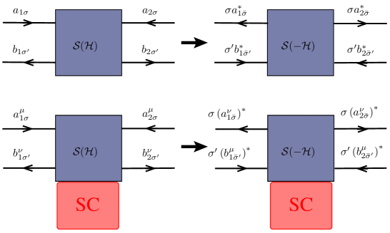
Figure 1: Microreversibility operating on a two-terminal ${\cal S}$-matrix in the absence (top) and in the presence of superconductivity (bottom). The scattering amplitudes $a$ and $b$ depend on spin indices, $\sigma=\uparrow(+1)$, $\downarrow(-1)$, quasiparticle indices, $\mu=e(+1)$, $h(-1)$ and terminal indices 1 and 2. Time-reversal implies inverting the particle’s momentum, spin and quasiparticle isospin, as well as magnetic fields and fluxes.

Reciprocity relations for ${\cal S}$ follow directly from microreversibility But86 . They read zha05 ,

$${\cal S}({\cal H})=\sigma^{(y)}\,{\cal S}^{\rm T}(-{\cal H})\,\sigma^{(y)}\,,$$ (6)

where $\sigma^{(y)}$ is a Pauli matrix acting in spin space, and “^T” indicates the matrix transpose of spin, transport channel and (with superconductivity) quasiparticle indices. Included in Eq. (6) is the relation ${\cal S}(\cal H)={\cal S}^{\rm T}(-{\cal H})$ valid when the antiunitary TRS operator squares to 1 and SRS is not broken. Eq. (6) can be derived by constructing ${\cal S}$ first with scattering states $\phi_{n\sigma}({\cal H})$, then with their time-reversed $-i\sigma^{(y)}K\phi_{n\sigma}(-{\cal H})$, with the complex conjugation operator $K$, and equating the two results zha05 . Eq. (6) is intimately related to Kramers degeneracy, which in the presence of TRS (${\cal H}=0$) follows from the symmetry property $H=\sigma^{(y)}H^{*}\sigma^{(y)}$ of the Hamiltonian $H$. Specifying to half-integer-spin particles, it can equivalently be rewritten in a form that renders its connection to microreversibility more evident

$${\cal S}^{\mu\nu}_{i\sigma,j\sigma^{\prime}}({\cal H})=\sigma\sigma^{\prime}{\cal S}^{\nu\mu}_{j\bar{\sigma}^{\prime},i\bar{\sigma}}(-{\cal H})\,,$$ (7)

where $i,j$ are transport channel indices, $\mu,\nu=e,h$ are quasiparticle indices and $\bar{\sigma}=-\sigma$ are spin indices.

Further relations can be constructed by combining Eqs. (6) and (7) with additional symmetries of the ${\cal S}$-matrix. The latter are obtained by translating PHS and SLS of the Hamiltonian into symmetries of the ${\cal S}$-matrix. For this purpose, we use the relation Mahaux

$${\cal S}(\epsilon)=1+2\pi iW^{\dagger}(H-\epsilon-i\pi WW^{\dagger})^{-1}W\,,$$ (8)

between ${\cal S}$ and $H$, with a rectangular matrix $W$ that couples the scatterer to external leads. We consider first PHS. The presence of superconductivity requires to introduce electron and hole quasiparticles, and when PHS is present, the energy spectrum is symmetric about zero energy (taken as the chemical potential of the superconductor). With the convention of Eq. (4), PHS reads $H=-\sigma^{(y)}\tau^{(y)}H^{*}\sigma^{(y)}\tau^{(y)}$ caveat2b , with the minus-sign indicating how the symmetry of the energy spectrum differs from Kramers degeneracy. From this we obtain caveat3

$${\cal S}({\cal H})=\sigma^{(y)}\tau^{(y)}\,{\cal S}^{*}({\cal H})\,\sigma^{(y)}\tau^{(y)}\,.$$ (9)

Combining Eqs. (6) and (9) and paying attention to the ordering of spin-indices given in Eq. (5), one obtains,

$$\hskip-8.53581pt{\cal S}^{\mu\nu}_{i\sigma,j\sigma^{\prime}}({\cal H})\, = \,\left({\cal S}^{\bar{\mu}\bar{\nu}}_{i\sigma,j\sigma^{\prime}}({\cal H})\right)^{*}$$ (10)

$$= \,\sigma\sigma^{\prime}{\cal S}^{\nu\mu}_{j\bar{\sigma}^{\prime},i\bar{\sigma}}(-{\cal H})\,$$

$$= \,\sigma\sigma^{\prime}\left({\cal S}^{\bar{\nu}\bar{\mu}}_{j\bar{\sigma}^{\prime},i\bar{\sigma}}(-{\cal H})\right)^{*}\,.\qquad$$

where quasiparticle indices $\mu,\nu=+1(e),-1(h)$ when they appear as prefactors.

The reciprocity relations (6) and (9) for the ${\cal S}$-matrix are illustrated in Fig. 1. We defined the ${\cal S}$-matrix via the relation ${\cal S}\,{\bf a}={\bf b}$ between vectors ${\bf a}$ and ${\bf b}$ of components for incoming and outgoing quasiparticle flux amplitudes, respectively. Each component of these vectors corresponds to a given terminal, a transverse transport channel in that terminal, a spin orientation and, in the presence of superconductivity, a quasiparticle index. Complex conjugation in Fig. 1 and Eq.(6) occurs because TRS and PHS are represented by antiunitary operators, i.e. products of a unitary operator with complex conjugation.

We finally comment on SLS. The chiral Hamiltonian symmetry reads $H=-\eta^{(z)}\,H\,\eta^{(z)}$, with the Pauli matrix $\eta^{(z)}$ acting in sublattice space. For the scattering matrix, this translates into

$${\cal S}({\cal H},\epsilon)=\eta^{(z)}\,{\cal S}^{\dagger}({\cal H},-\epsilon)\,\eta^{(z)}\,,$$ (11)

where in contrast to earlier symmetry relations, we explicitly had to write the energy-dependence of the ${\cal S}$-matrix. Combining Eqs. (6) and (11), one obtains,

$$\hskip-8.53581pt{\cal S}^{mn}_{i\sigma,j\sigma^{\prime}}({\cal H},\epsilon)\, = \,mn\left({\cal S}^{nm}_{j\sigma^{\prime},i\sigma}({\cal H},-\epsilon)\right)^{*}$$ (12)

$$= \sigma\sigma^{\prime}{\cal S}^{nm}_{j\bar{\sigma}^{\prime},i\bar{\sigma}}(-{\cal H},\epsilon)\,$$

$$= \,mn\,\sigma\sigma^{\prime}\left({\cal S}^{mn}_{i\bar{\sigma},j\bar{\sigma}^{\prime}}(-{\cal H},-\epsilon)\right)^{*},\qquad$$

where we introduced sublattice indices $m,n=A(+1),B(-1)$.

IV Scattering approach to transport and formulation of the problem

We consider a multiterminal device connected to $i,j=1,2,\ldots N$ electrodes. The linear response relation is

$$\left(\begin{array}[]{c}J_{i}\\ I_{i}^{(0)}\\ I_{i}^{(x)}\\ I_{i}^{(y)}\\ I_{i}^{(z)}\end{array}\right) = \sum_{j}\left(\begin{array}[]{ccccc}\Xi_{ij}^{(00)}&\Gamma_{ij}^{(00)}&\Gamma_{ij}^{(0x)}&\Gamma_{ij}^{(0y)}&\Gamma_{ij}^{(0z)}\\ B_{ij}^{(00)}&G_{ij}^{(00)}&G_{ij}^{(0x)}&G_{ij}^{(0y)}&G_{ij}^{(0z)}\\ B_{ij}^{(x0)}&G_{ij}^{(x0)}&G_{ij}^{(xx)}&G_{ij}^{(xy)}&G_{ij}^{(xz)}\\ B_{ij}^{(y0)}&G_{ij}^{(y0)}&G_{ij}^{(yx)}&G_{ij}^{(yy)}&G_{ij}^{(yz)}\\ B_{ij}^{(z0)}&G_{ij}^{(z0)}&G_{ij}^{(zx)}&G_{ij}^{(zy)}&G_{ij}^{(zz)}\end{array}\right)\left(\begin{array}[]{c}T_{j}-T_{0}\\ V_{j}-V_{0}\\ \mu_{j}^{(x)}/e\\ \mu_{j}^{(y)}/e\\ \mu_{j}^{(z)}/e\\ \end{array}\right)\,,$$ (28)

between heat, $J_{i}$, electric, $I_{i}^{(0)}$ and spin, $I_{i}^{(\alpha)}$ currents on the one hand, and temperatures, $T_{j}$, voltages, $V_{j}$ and spin accumulations, $\mu_{j}^{(\alpha)}$ on the other.

The coefficients with superindices ⁽⁰⁰⁾ are the usual thermoelectric coefficients, while the coefficients $G^{(\alpha\beta)}$ are conductances and spin-dependent conductances, relating electric and spin currents to electric voltages and spin accumulations ada09 ; Bar07 . Finally, one has spin-Peltier matrix elements $\Gamma^{(0\beta)}$ connecting heat currents to spin accumulations and spin-Seebeck matrix elements $B^{(\alpha 0)}$ connecting spin currents to temperature differences footnote:spinmatrel . The resulting spin caloritronic (spin-Seebeck and spin-Peltier) effects have been investigated theoretically Dubi ; swi ; qi ; wang and experimentally uchida ; Slachter ; Flipse . As usual, we assume that there is no spin relaxation in the terminals where spin currents are measured, so that the latter are well defined. Our goal is to determine reciprocity relations between the elements of the Onsager matrix defined on the right-hand side of Eq. (28) in the ten symmetry classes discussed in Section II dys62 ; ver93 ; alt97 .

We will express the matrix elements of the Onsager matrix in Eq. (28) in terms of the ${\cal S}$-matrix. We discuss separately purely metallic systems and hybrid systems consisting of normal metallic components connected to superconductors.

IV.1 Purely metallic systems

Purely metallic systems fall in either one of the Wigner-Dyson or in one of the chiral classes. We start from the expression for electric current in Ref. [But86, ], extending it to account for heat and spin currents, e.g. along the lines of Refs. [But90, ; ada09, ]. This gives us the following linear relations between electric, heat and spin currents, on one hand, and voltages, temperatures and spin accumulations, on the other hand;

$$J_{i} = \frac{1}{h}\int_{-\infty}^{\infty}{\rm d}\epsilon\left(-\frac{\partial f}{\partial\epsilon}\right)\epsilon\,\sum_{j,\beta}[2N_{i}\delta_{0\beta}\delta_{ij}-\mathcal{T}^{(0\beta)}_{ij}(\epsilon)]\qquad$$ (29a)

$$\qquad\qquad\qquad\times[\mu_{j}^{(\beta)}+\delta_{0\beta}\,\epsilon(T_{j}-T_{0})/T_{0}]\,,$$

$$I_{i}^{(\alpha)} = \frac{e}{h}\int_{-\infty}^{\infty}{\rm d}\epsilon\left(-\frac{\partial f}{\partial\epsilon}\right)\sum_{j,\beta}[2N_{i}\delta_{\alpha\beta}\delta_{ij}-\mathcal{T}^{(\alpha\beta)}_{ij}(\epsilon)]\qquad$$ (29b)

$$\qquad\qquad\qquad\times[\mu_{j}^{(\beta)}+\delta_{0\beta}\,\epsilon(T_{j}-T_{0})/T_{0}]\,,$$

where the sums run over all terminal indices $i,j$ and all charge-spin indices $\alpha,\beta=0,x,y,z$. The electrochemical potential in terminal $j$ is $\mu_{j}^{(0)}=\mu_{\rm F}+eV_{j}$ with the applied voltage $V_{j}$ and $T_{0}$ is the base temperature about which the Fermi function $f=(\exp[\epsilon/T]+1)^{-1}$ is expanded. The spin accumulations $\mu_{j}^{(\beta)}$, $\beta\neq 0$, are one half times the $\beta$-components of the spin accumulation vector $\bm{\mu}_{j}$, giving the difference in chemical potential between the two spin species along the $\beta$ axis, e.g. $\mu_{j}^{(z)}=(\mu_{j}^{(\uparrow)}-\mu_{j}^{(\downarrow)})/2$. They are nonequilibrium spin accumulations whose origin is of little importance here.

In Eqs. (29), we introduced the spin-dependent transmission and reflection coefficients

$$\mathcal{T}_{ij}^{(\alpha\beta)}={\rm Tr}[({\cal S}_{ij})^{\dagger}\sigma^{(\alpha)}_{i}{\cal S}_{ij}\ \sigma^{(\beta)}_{j}],$$ (30)

where $\sigma^{(\alpha)}$, $\alpha=0,x,y,z$ are Pauli matrices ($\sigma^{(0)}$ is the identity matrix) and the trace is taken over both spin and transmission channel indices. Note the position of the Pauli matrices, where $\sigma^{(\alpha)}_{i}$ measures the spin in direction $\alpha$ as the electron exits the systems, while $\sigma^{(\beta)}_{j}$ measures it along $\beta$ as the electron enters the system Bar07 ; ada09 . These coefficients depend on the energy $\epsilon$ of the injected electrons, which we explicitly wrote in Eq. (29). Reciprocity relations for the Onsager matrix elements in purely metallic systems directly follow from combining Eqs. (29) with the transformation rules for the $\mathcal{T}_{ij}^{(\alpha\beta)}$ under microreversibility. Pauli matrices satisfy $\sigma^{(\alpha)}_{\eta\eta^{\prime}}=(-1)^{n_{\alpha}}\eta\eta^{\prime}\big{[}\sigma^{(\alpha)}_{\bar{\eta}\bar{\eta}^{\prime}}\big{]}^{*}$ with $n_{x,y,z}=1$ and $n_{0}=0$. Using this and Eq. (7) we obtain

$$\mathcal{T}_{ij}^{(\alpha\beta)}({\cal H},\epsilon)=(-1)^{n_{\alpha}+n_{\beta}}\,\mathcal{T}_{ji}^{(\beta\alpha)}(-{\cal H},\epsilon)\,.$$ (31)

Thus the reciprocity relation between spin-dependent transmission coefficients in Eq. (31) picks up a minus sign if the spin is resolved upon entering the system, and another if it is resolved upon leaving the system.

IV.2 Metallic systems with chiral symmetry

The chiral classes correspond to systems with a bipartite lattice, however currently no experiments are capable of measuring sublattice-resolved currents. Thus the charge and spin-transport is given by Eqs. (29,30), with the trace over channels supplemented by a trace over the sublattice indices (A and B sites). If one could measure sublattice isospin current, then one would have to add further Pauli matrices acting in sublattice space into Eqs. (30), leading to extra factors $(-1)^{n_{\alpha^{\prime}}+n_{\beta^{\prime}}}$ due to isospin in Eq. (31). We do not consider this possibility further, due to its lack of physical implementation.

A relevant consequence of SLS is however that from Eq. (12), we get ${\mathcal{T}}_{ij}^{(\alpha\beta)}(\epsilon)={\mathcal{T}}_{ji}^{(\beta\alpha)}(-\epsilon)$. Combining this with Eq. (31) we obtain

$$\mathcal{T}_{ij}^{(\alpha\beta)}({\cal H},\epsilon)\ = \ \mathcal{T}_{ji}^{(\beta\alpha)}({\cal H},-\epsilon)$$ (32)

$$= \ (-1)^{n_{\alpha}+n_{\beta}}\mathcal{T}_{ji}^{(\beta\alpha)}(-{\cal H},\epsilon)$$

$$= \ (-1)^{n_{\alpha}+n_{\beta}}\mathcal{T}_{ij}^{(\alpha\beta)}(-{\cal H},-\epsilon)\,.$$

These relations are strictly valid only insofar as leads are preserving SLS, meaning that they connect equally to both sublattice sites of each unit cell.

IV.3 Hybrid superconducting-normal metallic systems

Hybrid normal-metallic/superconducting systems have Andreev electron-hole scattering. This scattering may induce PHS, in which case the system falls in one of the four Altland-Zirnbauer symmetry classes in Table 1 alt97 .

To include Andreev scattering, one has to consider two kinds of quasiparticles (electrons and holes), which carry excitation energy $\pm\epsilon$ counted from the chemical potential of the superconductor $\mu_{\rm sc}$. These quasiparticles are converted into one another when they hit the superconductor. Ref. [Cla96, ] constructed a scattering theory of thermoelectric transport which include these effects. We need to include spin currents and accumulations.

To do this, we go back to the derivation of the scattering theory in terms of creation and annihilation operators acting on scattering states in the lead (see e.g. Ref. [Beenakker-review, ]). We write hole creation operators at energy $\varepsilon$, in terms of electron annihilation operators at energy $-\varepsilon$ as $\bm{c}^{\rm(h)in/out\dagger}_{i;n}(\varepsilon)=\bm{c}^{\rm(e)in/out}_{i;n}(-\varepsilon)$ with

$$\bm{c}^{\rm(h)in/out\dagger}_{i;n}=\left(\!\begin{array}[]{c}c^{\rm(h)in/out\dagger}_{i;n\uparrow}\\ c^{\rm(h)in/out\dagger}_{i;n\downarrow}\end{array}\!\right)\!,\ \ \bm{c}^{\rm(e)in/out}_{i;n}=\left(\!\begin{array}[]{c}c^{\rm(e)in/out}_{i;n\uparrow}\\ c^{\rm(e)in/out}_{i;n\downarrow}\end{array}\!\right)\,.$$ (37)

Here, $i$ gives the index of a transverse mode in the $n$th lead, while “in” and “out” indicate whether the wave in that mode is ingoing or outgoing. As these operators obey fermionic commutation relations, one has

$$\hskip-42.67912pt\bm{c}^{{\rm e;in}\dagger}_{i;n}(-\varepsilon)\,\bm{\sigma}^{(\alpha)}\,\bm{c}^{{\rm e;in}}_{i;n}(-\varepsilon)$$ (38)

$$= \bm{\sigma}_{0}\delta_{\alpha 0}-\bm{c}^{{\rm h;in}\dagger}_{i;n}(\varepsilon)\,\sigma^{\rm(\alpha)\rm T}\,\bm{c}^{{\rm h;in}}_{i;n}(\varepsilon)\,,$$

with a similar relation for outgoing waves. The transpose in the second term is due to the fact that we commuted the hole operators to ensure normal ordering. We then use the scattering matrix to write outgoing operators in terms of incoming ones. Contributions coming from the first term in Eq. (38) cancel each other. We find that the operator which gives the spin-current along axis $\alpha$ in the electron sector is $\sigma_{\alpha}$ [as in Eq. (30)], while it is $-\sigma^{\rm T}_{\alpha}$ in the hole sector. Recalling that we use the convention in Eqs. (4,5), we must also rotate the spin-current operator in the hole sector. It becomes $-\sigma^{(y)}\sigma^{(\alpha)\rm T}\sigma^{(y)}=(-1)^{n_{\alpha}+1}\sigma^{(\alpha)}$. Thus in this convention, we can write this spin-current operator compactly as $\mu^{n_{\alpha}+1}\sigma^{(y)}$ which works for both electrons ($\mu=1$) and holes ($\mu=-1$). From here on, quasiparticle indices $\mu,\nu=+1(e),-1(h)$ when they appear as prefactors.

This calculation in terms of creation and annihilation operators for electrons and holes gives us the scattering matrix formula that we desire. Assuming that the number of transport channels $N_{i}$ is the same for each quasiparticle species, Eqs. (29) is replaced by

$$J_{i} = \frac{1}{h}\int_{0}^{\infty}{\rm d}\epsilon\left(-\frac{\partial f}{\partial\epsilon}\right)\epsilon\,\sum_{j,\beta}\left\{[4N_{i}\delta_{ij}-\sum_{\mu,\nu}\mathcal{T}^{(\mu\nu;00)}_{ij}(\epsilon)]\,\delta_{0\beta}\,\epsilon(T_{j}-T_{0})/T_{0}-\sum_{\mu,\nu}\nu\,\mathcal{T}^{(\mu\nu;0\beta)}_{ij}(\epsilon)\mu_{j}^{(\beta)}\right\}\,,$$ (39a)

$$I_{i}^{(\alpha)} = \frac{e}{h}\int_{0}^{\infty}{\rm d}\epsilon\left(-\frac{\partial f}{\partial\epsilon}\right)\sum_{j,\beta}\left\{[4N_{i}\delta_{\alpha\beta}\delta_{ij}-\sum_{\mu,\nu}\mu\nu\,\mathcal{T}^{(\mu\nu;\alpha\beta)}_{ij}(\epsilon)]\mu_{j}^{(\beta)}-\sum_{\mu,\nu}\mu\,\mathcal{T}^{(\mu\nu;\alpha 0)}_{ij}(\epsilon)\,\delta_{0\beta}\,\epsilon(T_{j}-T_{0})/T_{0}\right\}\,,\qquad$$ (39b)

where the integrals now go over a range of positive excitation energies Cla96 and we defined $\mu_{j}^{(0)}=e(V_{j}-V_{\rm sc})$, i.e. voltages are measured from the superconducting voltage $V_{\rm sc}=\mu_{\rm sc}/e$. We also introduced the spin-dependent, quasi-particle resolved transmission coefficients

$$\mathcal{T}_{ij}^{(\mu\nu;\alpha\beta)} = \ \mu^{n_{\alpha}}\,\nu^{n_{\beta}}\ {\rm Tr}\left[({\cal S}_{ij}^{\mu\nu})^{\dagger}\sigma^{(\alpha)}_{i}{\cal S}_{ij}^{\mu\nu}\sigma^{(\beta)}_{j}\right]$$ (40)

where ${\cal S}_{ij}^{\mu\nu}$ is the block of the ${\cal S}$-matrix corresponding to the transmission of a quasiparticle of type $\nu=e,h$ in lead $j$ to a $\mu$-quasiparticle in lead $i$.

Symmetry class		Seebeck-Peltier Onsager relations
		from microreversibility
Wigner-Dyson	A (unitary)	$B_{ij}^{(\beta 0)}({\cal H})T_{0}=(-1)^{n_{\beta}}\Gamma_{ji}^{(0\beta)}(-{\cal H})$
	AI (orthog.)	$B_{ij}^{(\beta 0)}T_{0}=\Gamma_{ji}^{(0\beta)}\propto\delta_{0\beta}$
	AII (sympl.)	$B_{ij}^{(\beta 0)}T_{0}=(-1)^{n_{\beta}}\Gamma_{ji}^{(0\beta)}$
Chiral	AIII(unitary)	$B_{ij}^{(\beta 0)}({\cal H})T_{0}=(-1)^{n_{\beta}}\Gamma_{ji}^{(0\beta)}(-{\cal H})$
	BDI (orthog.)	$B_{ij}^{(\beta 0)}T_{0}=\Gamma_{ji}^{(0\beta)}\propto\delta_{0\beta}$
	CII (sympl.)	$B_{ij}^{(\beta 0)}T_{0}=(-1)^{n_{\beta}}\Gamma_{ji}^{(0\beta)}$
Altland-Zirnbauer	D	$B_{ij}^{(\beta 0)}({\cal H})T_{0}=(-1)^{n_{\beta}}\Gamma_{ji}^{(0\beta)}(-{\cal H})$
	C	$B_{ij}^{(\beta 0)}({\cal H})T_{0}=\Gamma_{ji}^{(0\beta)}(-{\cal H})$
	DIII	$B_{ij}^{(\beta 0)}T_{0}=(-1)^{n_{\beta}}\Gamma_{ji}^{(0\beta)}$
	CI	$B_{ij}^{(\beta 0)}T_{0}=\Gamma_{ji}^{(0\beta)}\propto\delta_{0\beta}$

Table 3: The Onsager reciprocity relations arising from microreversibility and which involve the Peltier and spin-Peltier matrix elements, $\Gamma^{(0\beta)}$, and the Seebeck and spin-Seebeck matrix elements, $B^{(\beta 0)}$. These relations, combined with those due to PHS or SLS in Table 5, give the complete set of Onsager relations for each symmetry class.

The main novelty brought about by superconductivity is that the elements of the Onsager matrix now depend on Andreev processes via hybrid transmission coefficients $\mathcal{T}_{ij}^{(eh;\alpha\beta)}$ and $\mathcal{T}_{ij}^{(he;\alpha\beta)}$, which contribute differently to heat versus electric and spin currents — see in particular the last terms in Eqs. (39a) and (39b). From Eq. (7) one obtains

$$\mathcal{T}_{ij}^{(\mu\nu;\alpha\beta)}({\cal H},\epsilon)=(-1)^{n_{\alpha}+n_{\beta}}\mathcal{T}_{ji}^{(\nu\mu;\beta\alpha)}(-{\cal H},\epsilon)\,,$$ (41)

which extends Eq. (31) to include superconductivity.

Eq. (41) applies to any hybrid system, regardless of whether PHS is present or not. If additionally, the system has unbroken PHS, then the scattering matrix obeys Eq. (9), i.e. ${\cal S}^{\mu\nu}({\cal H})=\mu\nu\,\sigma^{(y)}[{\cal S}^{\bar{\mu}\bar{\nu}}({\cal H})]^{*}\sigma^{(y)}$, where, as before, $\mu,\nu=+1(e),-1(h)$. (Ref. [Cla96, ] has this formula for SRS, where ${\cal S}^{*}$ commutes with $\sigma^{(y)}$). We substitute this into Eq. (41), and then substitute $\sigma^{(y)}\sigma^{(\alpha)}\sigma^{(y)}=(-1)^{n_{\alpha}}\sigma^{(\alpha)\rm T}$. Observing that the trace is invariant under the transpose of its argument, we find that PHS gives

$$\mathcal{T}_{ij}^{(\mu\nu;\alpha\beta)}({\cal H},\epsilon)\ = \ \mathcal{T}_{ij}^{(\bar{\mu}\bar{\nu};\alpha\beta)}({\cal H},\epsilon)$$ (42)

$$= \ (-1)^{n_{\alpha}+n_{\beta}}\,\mathcal{T}_{ji}^{(\nu\mu;\beta\alpha)}(-{\cal H},\epsilon)$$

$$= \ (-1)^{n_{\alpha}+n_{\beta}}\,\mathcal{T}_{ji}^{(\bar{\nu}\bar{\mu};\beta\alpha)}(-{\cal H},\epsilon)\,.\qquad$$

V Onsager relations

Eqs. (29), (31), (39), (41) and (42) are all we need to derive reciprocity relations between the coefficients of the Onsager matrix in Eq. (28). Tables 3, 4 and 5 provide a complete list of all Onsager reciprocity relations for coupled electric, thermoelectric and spin transport in single-particle Hamiltonian systems. The Onsager relations which can be derived from microreversibility are divided into two sets. Firstly, Table 3 gives the Peltier/Seebeck relations, between coefficients $\Gamma^{(0\beta)}$ and $B^{(\beta 0)}$. Secondly Table 4 gives the reciprocity relations for conductances $G_{ij}^{(\alpha\beta)}$, $\Xi_{ij}^{(\alpha\beta)}$. As an example, we note that for both the Wigner-Dyson and chiral orthogonal classes, the presence of SRS imposes $\mathcal{T}_{ij}^{(\alpha\beta)}=\mathcal{T}_{ij}^{(00)}\delta_{\alpha\beta}$, while TRS gives $\mathcal{T}_{ij}^{(\alpha\beta)}=\mathcal{T}_{ji}^{(\beta\alpha)}$. Therefore, when both symmetries are present in those classes, $X_{ij}^{(\alpha\beta)}=X_{ji}^{(\alpha\beta)}$, for $X=\Xi$, $\Gamma$, $B$ and $G$. In addition there are those Onsager relations which can be derived from either the conservation of quasiparticle species (absence of Andreev processes turning e into h, and vice-versa), or from the presence of PHS or SLS. They are listed in Table 5.

Symmetry class		Onsager relations between conductances, $X=G,\Xi$
		from microreversibility
Wigner-Dyson	A (unitary)	$X_{ij}^{(\alpha\beta)}({\cal H})=(-1)^{n_{\alpha}+n_{\beta}}X_{ji}^{(\beta\alpha)}(-{\cal H})$
	AI (orthog.)	$X_{ij}^{(\alpha\beta)}=X_{ji}^{(\beta\alpha)}\propto\delta_{\alpha\beta}$
	AII (sympl.)	$X_{ij}^{(\alpha\beta)}=(-1)^{n_{\alpha}+n_{\beta}}X_{ji}^{(\beta\alpha)}$
Chiral	A III(unitary)	$X_{ij}^{(\alpha\beta)}({\cal H})=(-1)^{n_{\alpha}+n_{\beta}}X_{ji}^{(\beta\alpha)}(-{\cal H})$
	BDI (orthog.)	$X_{ij}^{(\alpha\beta)}=X_{ji}^{(\beta\alpha)}\propto\delta_{\alpha\beta}$
	CII (sympl.)	$X_{ij}^{(\alpha\beta)}=(-1)^{n_{\alpha}+n_{\beta}}X_{ji}^{(\beta\alpha)}$
Altland-Zirnbauer	D	$X_{ij}^{(\alpha\beta)}({\cal H})=(-1)^{n_{\alpha}+n_{\beta}}X_{ji}^{(\beta\alpha)}(-{\cal H})$
	C	$X_{ij}^{(\alpha\beta)}({\cal H})=X_{ji}^{(\beta\alpha)}(-{\cal H})$
	DIII	$X_{ij}^{(\alpha\beta)}=(-1)^{n_{\alpha}+n_{\beta}}X_{ji}^{(\beta\alpha)}$
	CI	$X_{ij}^{(\alpha\beta)}=X_{ji}^{(\beta\alpha)}\propto\delta_{\alpha\beta}$

Table 4: The Onsager reciprocity relations arising from microreversibility and which involve the electrical and spin-dependent conductances $G^{(\alpha\beta)}$ and the heat conductance $\Xi^{(00)}$, These relations, combined with those due to PHS or SLS in Table 5, give the complete set of Onsager relations for each symmetry class.

Some important features are that (i) in multiterminal devices one needs to consider conductance, Seebeck and Peltier matrices, and the reciprocity relations require to take their transpose, the latter operation being tantamount to momentum inversion as required by microreversibility, (ii) spin transport introduces additional minus signs everytime a spin is measured, (iii) exact PHS leads to the disappearance of thermoelectric and spin caloritronic effects, (iv) at half-filling, exact SLS leads to the disappearance of thermoelectric but not spin caloritronic effects.

That thermoelectric and spin caloritronic effects vanish in the presence of PHS directly follows from Eq. (40) that transmission coefficients satisfy $\mathcal{T}_{ij}^{(\mu\nu;\alpha\beta)}=\mathcal{T}_{ij}^{(\bar{\mu}\bar{\nu};\alpha\beta)}$ when PHS is strictly enforced. This gives in particular $\sum_{\nu}\nu\mathcal{T}_{ij}^{(\mu\nu;\alpha\beta)}=\sum_{\mu}\mu\mathcal{T}_{ij}^{(\mu\nu;\alpha\beta)}=0$ which, together with Eq. (39), directly gives $B_{ij}^{(0\alpha)}({\cal H})=\Gamma_{ij}^{(\alpha 0)}({\cal H})=0$.

The vanishing of thermoelectric effects with PHS is reminiscent of Mott’s relation, giving that the Seebeck coefficient is proportional to the derivative of the conductance at the Fermi energy – the latter vanishes in PHS systems. Still, hybrid normal metallic/superconducting systems often exhibit larger thermoelectric effects than their purely metallic counterpart, which typically happens in the crossover regime between Altland-Zirnbauer and Wigner-Dyson symmetry classes. For the crossover systems described in Table 2, thermoelectric effects can be quite large Eom98 ; Cad09 ; Par03 .

We close this section with two comments on SLS at half-filling, when the chemical potential is at zero energy. Systems in the chiral symmetry classes have transmission coefficients with extra symmetries given in Eq. (32). The latter have important consequences for the symmetry of transport, if the trace over the sublattice index in Eq. (30) involves only pairs of sublattice sites, i.e. when SLS is not broken by the terminals. When this is the case, the first and second equalities in Eq. (32), together with Eqs. (29), give $G_{ij}^{(\alpha\beta)}({\cal H})=G_{ji}^{(\beta\alpha)}({\cal H})$ and $G_{ij}^{\alpha\beta}({\cal H})=(-1)^{n_{\alpha}+n_{\beta}}G_{ji}^{\beta\alpha}(-{\cal H})$ respectively, where we recall that $n_{0}=0$ and $n_{x,y,z}=1$. We obtain identical results for $\Xi_{ij}^{(00)}$, and thus conclude that

$$G_{ij}^{(\alpha\beta)}({\cal H})=(-1)^{n_{\alpha}+n_{\beta}}G_{ij}^{(\alpha\beta)}(-{\cal H}),$$

$$\Xi_{ij}^{(00)}({\cal H})=\Xi_{ij}^{(00)}(-{\cal H})\,.$$ (43)

We see that charge-conductance, spin-conductances and thermal conductance are even in external fields, ${\cal H}$, irrespective of how many terminals the device has. This is in contrast to normal-metallic systems without SLS, where only two-terminal devices have conductances even in ${\cal H}$. In contrast, spin-to-charge and charge-to-spin conversion are strictly odd in ${\cal H}$, irrespective of how many terminals the device has.

Symmetry class		Special additional relations
Wigner	A (unitary)	$B_{ij}^{(00)}({\cal H})=B_{ji}^{(00)}(-{\cal H})$
-Dyson	AI (orthog.)	$B_{ij}^{(00)}=B_{ji}^{(00)}$
	AII (sympl.)	$B_{ij}^{(00)}=B_{ji}^{(00)}$
Chiral	AIII(unitary)	$X_{ij}^{(\alpha\beta)}({\cal H})=X_{ij}^{(\alpha\beta)}(-{\cal H})$ for $X=\{G,\Xi\}$,  $B_{ij}^{(\beta 0)}({\cal H})=B_{ij}^{(\beta 0)}(-{\cal H})$,   $B_{ij}^{(00)}({\cal H})=0$
(half-filling only)	BDI (orthog.)	$B_{ij}^{(\beta 0)}=\Gamma_{ij}^{(0\beta)}=0$
	CII (sympl.)	$B_{ij}^{(\beta 0)}=\Gamma_{ij}^{(0\beta)}=0$
Altland	D	$B_{ij}^{(\beta 0)}({\cal H})=\Gamma_{ij}^{(0\beta)}({\cal H})=0$
-Zirnbauer	C	$B_{ij}^{(\beta 0)}({\cal H})=\Gamma_{ij}^{(0\beta)}({\cal H})=0$
	DIII	$B_{ij}^{(\beta 0)}=\Gamma_{ij}^{(0\beta)}=0$
	CI	$B_{ij}^{(\beta 0)}=\Gamma_{ij}^{(0\beta)}=0$

Table 5: Additional reciprocity relations induced by the conservation of each quasiparticle species (absence of Andreev reflection from e to h), or by the presence of PHS or SLS, to be added to the Onsager relations in Tables 3 and 4. The additional relation between $B$ and its transpose (and an identical one, not listed here, between $\Gamma$ and its transpose) in the Wigner-Dyson classes was first noticed in Ref. [But90, ], which allows one to express the Seebeck/Peltier relation of Table 3 in two different but equivalent ways. Thermoelectric and spin caloritronic effects disappear identically in the presence of PHS. The relations in the chiral classes correspond to transport at half-filling, $E=0$. Outside of this regime, chiral systems have the same relations as in the (corresponding) Wigner-Dyson classes.

Turning to thermoelectric and spin caloritronic effects, the first equality in Eq. (32) gives $B_{ij}^{(\beta 0)}({\cal H})\,T_{0}=-\Gamma_{ji}^{(0\beta)}({\cal H})$, while the second equality in Eq. (32) gives us the usual relation $B_{ij}^{(\beta 0)}({\cal H})\,T_{0}=(-1)^{n_{\beta}}\Gamma_{ji}^{(0\beta)}(-{\cal H})$. Thus we can conclude that

$$B_{ij}^{(\beta 0)}({\cal H})=B_{ij}^{(\beta 0)}(-{\cal H})\ \hbox{ for }\ \beta\in\{x,y,z\},$$ (44a)

$$B_{ij}^{(00)}({\cal H})=0,$$ (44b)

with identical relations for $\Gamma_{ij}^{(0\beta)}$. Additionally, any system with PHS has no thermoelectric nor spin caloritronic response. Looking at Table 1 we see that only the AIII symmetry class has SLS without PHS. Thus in this symmetry class, the spin-Seebeck and spin-Peltier coefficients are even functions of the external field, ${\cal H}$, while the usual Seebeck and Peltier coefficients vanish identically.

We stress, however, that the analysis leading to Eqs. (V) and (44) holds only at half-filling, when the Fermi function in Eq. (29) is symmetric around $\epsilon=0$, and, perhaps physically more important, when the terminals do not break SLS. This requires leads to be connected with equal strength to both sublattice sites in each unit cell.

VI Examples of reciprocity relations in spintronics and spin caloritronics

VI.1 Spin Hall and inverse spin Hall effects

As a first example of the reciprocities we derived, we discuss the spin Hall han05 ; Bar07 ; DP71 ; eng07 ; Kato and the inverse spin Hall han05 ; val06 ; Sai06 ; Kim07 ; Sek08 ; Liu11 ; ada09 effects. The two effects are sketched in Fig. 2. In the spin Hall effect, Fig. 2a, one passes an electric current between terminals 1 and 2 and measures the spin current between terminals 3 and 4. The voltages at terminals 3 and 4 are set such that no current flows through them on time average. In the limit of large and identical number of channels in each terminal, $N\gg 1$, the voltages $V_{3}$ and $V_{4}$ lie almost exactly in the middle between $V_{1}$ and $V_{2}$, $V_{3,4}\simeq(V_{1}+V_{2})/2$ for ballistic systems Bar07 . We assume that this is the case here, and set $V_{1}=V/2$, $V_{2}=-V/2$, $V_{3,4}=0$.

The presence of spin-orbit coupling inside the system generates a spin current flowing through the transverse terminals. When all terminals are at zero temperature, these currents are given by

$$I_{3}^{(\alpha)} = -\frac{e^{2}V}{2h}(\mathcal{T}_{31}^{(\alpha 0)}-\mathcal{T}_{32}^{(\alpha 0)})\,,$$ (45a)

$$I_{4}^{(\alpha)} = -\frac{e^{2}V}{2h}(\mathcal{T}_{41}^{(\alpha 0)}-\mathcal{T}_{42}^{(\alpha 0)})\,.$$ (45b)

In the inverse spin Hall effect, Fig. 2b, there is no voltage bias, but instead terminals 3 and 4 have opposite spin accumulations. In an idealized situation they will be $\pm\mu^{(\alpha)}/2$. Spin-orbit coupling converts this spin accumulation into a transverse electric current. The currents in terminals 1 and 2 read

$$I_{1}^{(0)} = -\frac{e\mu^{(\alpha)}}{2h}(\mathcal{T}_{13}^{(0\alpha)}-\mathcal{T}_{14}^{(0\alpha)})\,,$$ (46a)

$$I_{2}^{(0)} = -\frac{e\mu^{(\alpha)}}{2h}(\mathcal{T}_{23}^{(0\alpha)}-\mathcal{T}_{24}^{(0\alpha)})\,.$$ (46b)

In both cases, the Hall part of the currents, flowing between 3 and 4 in the case of the spin Hall effect and betwee 1 and 2 in the case of the inverse spin Hall effect, is given by the difference in the two currents. We define spin Hall and inverse spin Hall conductances as $I_{sHe}^{(\alpha)}=I_{3}^{(\alpha)}-I_{4}^{(\alpha)}=G_{\rm sHe}V$ and $I_{isHe}^{(0)}=I_{2}^{(0)}-I_{1}^{(0)}=G_{\rm isHe}\,\mu^{(\alpha)}/e$. One obtains

$$G_{\rm sHe} = -\frac{e^{2}}{2h}(\mathcal{T}_{31}^{(\alpha 0)}-\mathcal{T}_{32}^{(\alpha 0)}-\mathcal{T}_{41}^{(\alpha 0)}+\mathcal{T}_{42}^{(\alpha 0)})\,,\qquad$$ (47a)

$$G_{\rm isHe} = -\frac{e^{2}}{2h}(\mathcal{T}_{23}^{(0\alpha)}-\mathcal{T}_{24}^{(0\alpha)}-\mathcal{T}_{13}^{(0\alpha)}+\mathcal{T}_{14}^{(0\alpha)})\,.$$ (47b)

Together with Eq. (31), Eq. (47a) gives $G_{\rm sHe}=G_{\rm isHe}$. The reciprocity between direct and inverse spin Hall conductances is exact and does not require sample averaging, as sometimes claimed han05 .

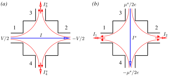
Figure 2: Sketch of a four-terminal spin-Hall (a) and inverse spin Hall (b) experiment. (a) In the spin Hall effect, an electric current (blue arrow) generates transverse spin currents (red) via the action of spin-orbit coupling. (b) In the inverse spin Hall effect spin accumulations inject a spin current (blue arrow) which, in the presence of spin-orbit coupling, generates a transverse electric current (red).

VI.2 Reciprocity between spin injection and magnetoelectric spin currents

For a spin index $\beta=0$, Eqs. (31) and (41) establish the reciprocity between magnetoeletric effects generating spin currents from electric voltage biases and spin injection from spin accumulations in the terminals, a special case of which is the above-discussed spin Hall effect/inverse spin Hall effect reciprocity. In the presence of TRS, it has already been observed that one consequence of Eq. (7) is that no spin current can be magnetoelectrically generated in a two-terminal device if the exit lead carries a single (spin-degenerate) transport channel. The reciprocity relations of Eqs. (31) and (41) further impose that a spin injection from such a terminal is incapable of generating an electric current, unless one goes to the nonlinear regime stano2 . This seems not to have been noted so far.

VI.3 Spin Seebeck and spin Peltier coefficients in two-terminal geometries

In two-terminal geometries, the electric conductance is symmetric in TRS breaking fields, which follows from current conservation or gauge invariance, together with the symmetry of electric reflection coefficients, $G_{ii}^{(00)}({\cal H})=G_{ii}^{(00)}(-{\cal H})$ (see e.g. Ref. [But86, ]). Including spin-transport, the unitarity of the scattering matrix further results in spin-current conservation and generalized gauge invariance,

$$\sum_{i}\left(2N_{i}\delta_{0\alpha}\delta_{ij}-\mathcal{T}_{ij}^{(0\alpha)}\right)=0\,,\qquad$$

$$\sum_{j}\left(2N_{i}\delta_{0\alpha}\delta_{ij}-\mathcal{T}_{ij}^{(\alpha 0)}\right)=0\,,$$ (48)

under the assumption that the number of transport channels coupling the system to external reservoirs is spin-independent. In two-terminal geometries this gives

$$B_{11}^{(\beta 0)}+B_{12}^{(\beta 0)}=B_{21}^{(\beta 0)}+B_{22}^{(\beta 0)}=0\,,\qquad$$

$$\Gamma_{11}^{(0\beta)}+\Gamma_{21}^{(0\beta)}=\Gamma_{12}^{(0\beta)}+\Gamma_{22}^{(0\beta)}=0\,.$$ (49)

However, unlike for the charge conductance, the thermoelectric reflection coefficients can have both a symmetric and an antisymmetric component. This is directly seen from the expression

$$B_{ii}^{(\beta 0)}({\cal H})=\frac{-e}{h}\int{\rm d}\epsilon\left(-\frac{\partial f}{\partial\epsilon}\right)\,\frac{\epsilon}{T_{0}}\,\mathcal{T}^{(\beta 0)}_{ii}({\cal H},\epsilon)$$ (50)

for the spin Seebeck reflection coefficient. For example for $\beta=z$, the spin-dependent transmission coefficient in the integrand reads

$${\mathcal{T}}_{ii}^{(z0)} = {\mathcal{T}}_{\rm s}^{(z0)}-{\mathcal{T}}_{a}^{(z0)}\,,$$ (51a)

$${\mathcal{T}}_{\rm s}^{(z0)} \equiv T_{i\uparrow,i\downarrow}-T_{i\downarrow,i\uparrow}\,$$ (51b)

$${\mathcal{T}}_{a}^{(z0)} \equiv T_{i\uparrow,i\uparrow}-T_{i\downarrow,i\downarrow}\,,$$ (51c)

which, from Eq. (7) has both symmetric, ${\mathcal{T}}_{\rm s}^{(z0)}({\cal H})={\mathcal{T}}_{\rm s}^{(z0)}(-{\cal H})$, and antisymmetric, ${\mathcal{T}}_{a}^{(z0)}({\cal H})={\mathcal{T}}_{a}^{(z0)}(-{\cal H})$ components.

An interesting example is provided by a two-terminal system with a well-defined spin quantization axis. This is the case, for example, for a system without spin-orbit coupling in a uniform Zeeman field, for two-dimensional systems with both Rashba and Dresselhaus spin-orbit interactions of equal strengths egues , or for a system with pure $\,\vec{l}\cdot\vec{s}\,$ spin-orbit coupling. Without loss of generality we define the spin quantization axis as the $z$-axis. Then ${\cal S}$ commutes with $\sigma^{(z)}$, i.e. it is diagonal in spin space. From Eq. (30), we find that ${\mathcal{T}}_{ij}^{(z0)}({\cal H})={\mathcal{T}}_{ij}^{(0z)}({\cal H})$ and ${\mathcal{T}}_{ij}^{(\alpha 0)}({\cal H})=0$ when $\alpha=x,y$. Combining this with Eqs. (VI.3), we have ${\mathcal{T}}_{12}^{(z0)}({\cal H})={\mathcal{T}}_{12}^{(0z)}({\cal H})={\mathcal{T}}_{21}^{(z0)}({\cal H})={\mathcal{T}}_{21}^{(0z)}({\cal H})$. Thus

$$B^{(z0)}_{12}({\cal H})T_{0}=\Gamma^{(0z)}_{12}({\cal H})\,,$$ (52)

with $\Gamma^{(0\alpha)}_{\rm 12}({\cal H})=0$ when $\alpha=x,y$. Next we recall that the Seebeck-Peltier Onsager relations contain an extra minus sign for spin caloritronic effects compared to usual thermoelectric effects (see Table 3). This extra minus sign means that $B^{(z0)}_{\rm 12}$ and $\Gamma^{(0z)}_{\rm 12}$ are odd in ${\cal H}$, while $B^{(00)}_{\rm 12}$ and $\Gamma^{(00)}_{\rm 12}$ are even in ${\cal H}$. Thus any two-terminal system with a spin-quantization axis will have spin-Seebeck and spin-Peltier effects which are odd functions of TRS breaking fields, while the normal Seebeck and Peltier effects are even function of those fields.

VII Examples of reciprocity relations in thermoelectricity with hybrid systems

Thermoelectric effects in the presence of superconductivity, in particular the thermopower $S=-B^{(00)}/G^{(00)}$ and thermal conductance $\Xi^{(00)}$, have attracted quite some experimental Eom98 ; Cad09 ; Par03 and theoretical interest Cla96 ; Vir04 ; Tit08 ; Jac10 ; Eng11 ; Sev00 ; Bez03 . However, the exact form that the Seebeck-Peltier Onsager reciprocity relation takes has never been clarified, despite the fact that two-terminal devices with superconductors usually exhibit odd Seebeck coefficients $S({\cal H})=-S(-{\cal H})$, in stark contrast with Mott’s relation Ash67 . Mott’s relation between the thermopower of metallic systems at low temperature and the energy derivative of the conductance at the Fermi energy, reads

$$S=-\frac{\pi^{2}k_{\rm B}^{2}T}{3e}\partial_{E}{\rm ln}G(E_{\rm F})\,,$$ (53)

and thereby indicates that $S$ should be even in ${\cal H}$. This evenness of $S$ is confirmed by the scattering theory for metallic systems But90 . In this section we provide examples clarifying this issue using scattering theory to show that $S$ can have any symmetry under ${\cal H}\to-{\cal H}$ when superconductors are present.

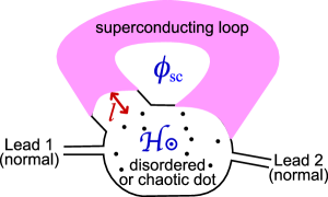
Figure 3: An Andreev interferometer: two-terminal hybrid system with two normal metallic/superconducting contacts with tunable superconducting phase difference $\phi_{\rm SC}$. The latter, together with a systematic delay (indicated by the extra length $\ell$) towards one of the superconducting contacts can break PHS and generate finite thermoelectric effects Jac10 . The particular symmetry class in which the system falls is given by how much magnetic field ${\cal H}$ and how much spin-orbit coupling there is in the dot, see Table 1.

VII.1 Seebeck–Peltier reciprocity relation

Andreev scattering strongly influences the Seebeck–Peltier reciprocity relation between $\Gamma$ and $B$ coefficients. Comparison of the last terms in Eqs. (39a) and (39b) shows that the $ee$ and $hh$ terms in $\Gamma$ and $B$ have the same sign, while the $eh$ and $he$ terms acquire a relative minus sign. This breaks one of the Onsager relations between Peltier and Seebeck coefficients. For metallic systems, one has both $B_{ij}^{(00)}({\cal H})T_{0}=\Gamma_{ji}^{(00)}(-{\cal H})$ and $B_{ij}^{(00)}({\cal H})T_{0}=\Gamma_{ij}^{(00)}({\cal H})$ But90 , however, with superconductivity, only $B_{ij}^{(00)}({\cal H})T_{0}=\Gamma_{ji}^{(00)}(-{\cal H})$ holds.

When PHS strictly holds, however, $\sum_{\nu}\nu{\mathcal{T}}_{ij}^{(\mu\nu;\alpha\beta)}=\sum_{\mu}\mu{\mathcal{T}}_{ij}^{(\mu\nu;\alpha\beta)}=0$ and both $\Gamma$- and $B$-coefficients vanish identically, regardless of the temperature. However, interesting thermoelectric effects appear in hybrid systems when PHS is broken. Focusing on a two-terminal geometry, as depicted in Fig. 3, Eq. (39) can be rewritten in the form

$$\left(\begin{array}[]{c}J\\ I\end{array}\right) = \left(\begin{array}[]{cc}\Xi&\Gamma\\ B&G\end{array}\right)\left(\begin{array}[]{c}\Delta T\\ \Delta V\end{array}\right)\,,$$ (60)

which depends only on the voltage and temperature differences between the two normal reservoirs. The two-terminal thermoelectric coefficients are given by

$$G = G^{(00)}_{11}-{\big{(}G^{(00)}_{11}+G^{(00)}_{12}\big{)}\big{(}G^{(00)}_{11}+G^{(00)}_{21}\big{)}\over G_{11}^{(00)}+G_{22}^{(00)}+G_{12}^{(00)}+G_{21}^{(00)}}\,,\qquad$$ (61a)

$$\Xi = \Xi^{(00)}_{11}-{\big{(}\Gamma^{(00)}_{11}+\Gamma^{(00)}_{12}\big{)}\big{(}B^{(00)}_{11}+B^{(00)}_{21}\big{)}\over G_{11}^{(00)}+G_{22}^{(00)}+G_{12}^{(00)}+G_{21}^{(00)}}\,,$$ (61b)

$$B = B^{(00)}_{11}-{\big{(}G^{(00)}_{11}+G^{(00)}_{12}\big{)}\big{(}B^{(00)}_{11}+B^{(00)}_{21}\big{)}\over G_{11}^{(00)}+G_{22}^{(00)}+G_{12}^{(00)}+G_{21}^{(00)}}\,,$$ (61c)

$$\Gamma = \Gamma^{(00)}_{11}-{\big{(}\Gamma^{(00)}_{11}+\Gamma^{(00)}_{12}\big{)}\big{(}G^{(00)}_{11}+G^{(00)}_{21}\big{)}\over G_{11}^{(00)}+G_{22}^{(00)}+G_{12}^{(00)}+G_{21}^{(00)}}\,.$$ (61d)

in terms of the coefficients $X_{ij}^{(00)}$ ($X=G,B,\Gamma,\Xi$) defined by Eqs. (28) and (39).

It is then straightforward to see that the reciprocity relations read specifically

$$G(\mathcal{H}) = G(-\mathcal{H})\,,$$ (62a)

$$\Xi(\mathcal{H}) = \Xi(-\mathcal{H})\,,$$ (62b)

$$B(\mathcal{H})\;T_{0} = \Gamma(-\mathcal{H})\,.$$ (62c)

In particular the presence of superconductivity forces one to invert the sign of the TRS breaking field in the relation of Eq. (62c) between Seebeck and Peltier coefficients.

VII.2 Symmetry of the thermopower

The symmetry of the two-terminal thermopower, $S=-B^{(00)}/G^{(00)}$ is not specified in the presence of superconductivity Jac10 . The Seebeck coefficients read

$$B^{(00)}_{ij}({\cal H}) = \frac{2e}{hT_{0}}\int_{0}^{\infty}{\rm d}\varepsilon\,(-\partial_{\varepsilon}f)\,\varepsilon\,$$ (63)

$$\qquad\times\big{[}{\mathcal{T}}_{ij}^{(ee;00)}(\varepsilon,{\cal H})+{\mathcal{T}}_{ij}^{(eh;00)}(\varepsilon,{\cal H})$$

$$\qquad\quad-{\mathcal{T}}_{ij}^{(he;00)}(\varepsilon,{\cal H})-{\mathcal{T}}_{ij}^{(hh;00)}(\varepsilon,{\cal H})\big{]}\,.\qquad$$

From this expression we see that thermoelectric effects vanish, $B^{(00)}_{ij}=0$, if PHS is enforced; we thus consider this equation in the absence of PHS. From Eq. (7) we know that ${\mathcal{T}}_{ii}^{(\mu\mu;00)}(\varepsilon,{\cal H})={\mathcal{T}}_{ii}^{(\mu\mu;00)}(\varepsilon,-{\cal H})$, while ${\mathcal{T}}_{ii}^{(eh;00)}(\varepsilon,{\cal H})={\mathcal{T}}_{ii}^{(he;00)}(\varepsilon,-{\cal H})$. Together with unitarity, $\sum_{j,\nu}{\mathcal{T}}_{ij}^{\mu\nu}(\varepsilon,{\cal H})=N_{i}^{\mu}$ and assuming that the number $N_{j}^{\mu}$ of transport channels depends neither on the quasiparticle type nor on the magnetic field, we readily obtain that $B^{(00)}_{ij}({\cal H})=B^{(00)}_{\rm even}({\cal H})+B^{(00)}_{\rm odd}({\cal H})$ is the sum of an even and an odd component,

$$B^{(00)}_{\rm even}({\cal H}) = \frac{2e}{hT_{0}}\int_{0}^{\infty}{\rm d}\varepsilon\,(-\partial_{\varepsilon}f)\,\varepsilon\,$$ (64a)

$$\times\big{[}{\mathcal{T}}_{ij}^{(ee;00)}(\varepsilon,{\cal H})-{\mathcal{T}}_{ij}^{(hh;00)}(\varepsilon,{\cal H})\big{]}\,,\qquad\quad$$

$$B^{(00)}_{\rm odd}({\cal H}) = \frac{2e}{hT_{0}}\int_{0}^{\infty}{\rm d}\varepsilon\,(-\partial_{\varepsilon}f)\,\varepsilon\,$$ (64b)

$$\times\big{[}{\mathcal{T}}_{ij}^{(eh;00)}(\varepsilon,{\cal H})-{\mathcal{T}}_{ij}^{(he;00)}(\varepsilon,{\cal H})\big{]}\,.$$

where $B^{(00)}_{\rm even}(-{\cal H})=B^{(00)}_{\rm even}({\cal H})$ and $B^{(00)}_{\rm odd}(-{\cal H})=-B^{(00)}_{\rm odd}({\cal H})$. In the absence of Andreev scattering, $B^{(00)}({\cal H})=B^{(00)}_{\rm even}({\cal H})$ is strictly even in two-terminal geometries, however Andreev scattering gives rise to an odd component. The asymmetric Andreev interferometers considered in Ref. [Jac10, ] were devised to render $B^{(00)}_{\rm odd}({\cal H})$ finite on mesoscopic average, which led to an antisymmetric thermopower in such systems. There are currently no known hybrid systems which have a finite-average $B^{(00)}_{\rm even}({\cal H})$. Recent theoretical works pointed out asymmetries in the thermopower of metallic systems in the presence of inelastic scattering, which is of interest because asymmetric thermopower may lead to more efficient thermal engines Sai11 ; San11 . Hybrid systems are examples of systems with purely elastic scattering and antisymmetric thermopower.

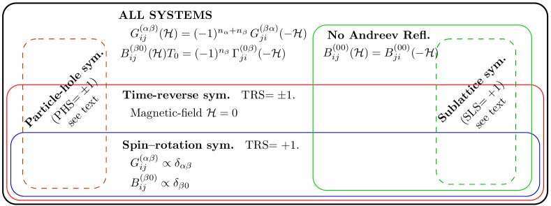
Figure 4: Venn diagram summarizing the Onsager relations we derived. Here $\alpha,\beta\in\{0,x,y,z\}$, $n_{0}=0$ and $n_{x}=n_{y}=n_{z}=1$. Any system obeys the relations given in all boxes it is within. For instance the Onsager relations for a generic system with time-reversal symmetry (TRS) read $G_{ij}^{(\alpha\beta)}=(-1)^{n_{\alpha}+n_{\beta}}G_{ji}^{(\beta\alpha)}$ and $B_{ij}^{(\beta 0)}\,T_{0}=(-1)^{n_{\beta}}\Gamma_{ji}^{(0\beta)}$, since TRS requires that any external magnetic field ${\cal H}=0$. If that system also had SRS, then the only nonzero coefficients are those with repeated upper-indices ($\alpha=\beta$ for $G$ and $\beta=0$ for $B$) for which $G_{ij}^{(\beta\beta)}=G_{ji}^{(\beta\beta)}$ and $B_{ij}^{(00)}\,T_{0}=\Gamma_{ji}^{(00)}$. If the system contains no Andreev reflection (i.e. no superconductors), one additionally has But90 $B_{ij}^{(00)}({\cal H})=B_{ji}^{(00)}(-{\cal H})$. In the case of PHS and SLS, the extra symmetry relations derived in the text are summarized in Table 5.

VII.3 Onset of thermoelectric effects upon breaking of PHS

Thermoelectric effects vanish identically in all Altland-Zirnbauer symmetry classes because of PHS. However in physical systems PHS is often at least partially broken, leading to finite thermoelectric effects. Here we show that the symmetry of such thermoelectric effects is subtly dependent on how PHS symmetry is broken.

To that end we consider the Andreev interferometer shown in Fig. 3. A two-terminal chaotic ballistic or disordered diffusive quantum dot is connected to a superconducting loop via two contacts. The superconducting phase difference at the two contacts can be tuned by a magnetic flux piercing the loop. There are two important time scales in the system, (i) the typical time $\tau_{\rm Andr}$ between two consecutive Andreev reflections at the superconducting contact, and (ii) the escape time $\tau_{\rm esc}$ to one of the normal leads. We additionally choose a special geometry where the average time to reach one of the two superconducting contacts from one of the normal leads is longer – this is achieved by an extra ballistic ”neck” of length $\ell$ between the cavity and the superconducting contact (see Fig. 3). Because of the neck, quasiparticles need an additional time delay $\delta\tau=\ell/v_{\rm F}$ to reach the left superconducting contact from a normal lead. Together with this time delay, a magnetic flux piercing the superconducting loop and making the superconducting phase difference $\phi_{\rm sc}$ finite also breaks PHS, thereby turning thermoelectric effects on Jac10 ; Eng11 .

Formally, PHS requires that $\tau_{\rm Andr}\to 0$, which practically means that $\tau_{\rm Andr}$ has to be smaller than any other time scale and any other inverse energy scale. When this is not the case, transport processes without any Andreev reflection exist, giving contributions to the conductance that fluctuate randomly in energy around the Fermi energy. This breaks PHS and leads for instance to finite, albeit relatively weak, thermopower Lan98 ; God99 . More generally, breaking PHS can be achieved in three different ways,

• rendering escape into the normal leads faster (for instance by widening the normal leads), until $\tau_{\rm esc}\sim\tau_{\rm Andr}$,
  

• raising the temperature until $(k_{`\rm B}T)^{-1}\sim\tau_{\rm Andr}$, or
  

• changing the flux through the superconducting loop so that $\phi_{\rm SC}\neq 0,\pi$, when the neck length $\ell$ is finite.

In case (i), a significant proportion of quasiparticles go from one normal lead to another without Andreev reflection. Then contributions to $\mathcal{T}_{ij}^{(\mu\mu;\alpha\beta)}({\cal H})$ which arise from processes without Andreev reflections will start to dominate thermoelectric transport, meaning $B^{(00)}_{\rm even}\gg B^{(00)}_{\rm odd}$ [as defined in Eq. (64)]. Thus, thermoelectric effects acquire the same symmetry as systems without SC contacts, i.e. they become predominantly even.

The situation is more complicated in case (ii), where both $\mathcal{T}_{ij}^{(\mu\mu;\alpha\beta)}({\cal H})$ and $\mathcal{T}_{ij}^{(\mu\overline{\mu};\alpha\beta)}({\cal H})$ have similar magnitude. In the absence of a neck, $\ell=0$, thermoelectric effects vanish on average and are dominated by mesoscopic fluctuations Jac10 ; Eng11 . An analysis of these mesoscopic fluctuations analogous to that in Ref. [Jac10, ] shows that there is no correlation between $B_{ij}^{(00)}({\cal H})$ and $B_{ji}^{(00)}(-{\cal H})$, so that the thermoelectric effects have no particular symmetry beyond the generic Onsager reciprocities given in Table 3. In particular, for a two terminal device $B^{(00)}_{\rm even}$ and $B^{(00)}_{\rm odd}$ are independent random variables with the same variance. Thus for a given Andreev interferometer (given disorder or cavity shape) either quantity could be positive or negative, and either could have a larger magnitude than the other.

Finally in case (iii), the physics changes completely. Due to the presence of a finite-sized neck, $\ell\neq 0$, and superconducting phase difference $\phi_{\rm sc}\neq 0,\pi$, the system develops a large average thermopower which is an odd function of the flux $\phi_{\rm sc}$ Vir04 ; Tit08 ; Jac10 ; Eng11 , with a much smaller even component coming from mesoscopic fluctuations Jac10 .

In summary depending on how particle-hole symmetry is broken, one gets a thermopower which is predominantly even in ${\cal H}$ [case (i)], predominantly odd in ${\cal H}$ [case (iii)], or which has no particular symmetry [case (ii)].

VIII Conclusions

We have derived a complete list of reciprocity relations for coupled electric, spin, thermoelectric and spin caloritronic transport effects in all ten symmetry classes for single-particle Hamiltonian systems. Several of these relations appeared in one way or another in earlier works, and the main novelties we found are (i) reciprocities in spintronics and spin caloritronics pick a number of additional minus signs reflecting spin current injection and measurement, (ii) a number of special relations have been listed in Table 5, which exist only in specific symmetry classes, (iii) we clarified the exact form of Onsager relations in the presence of superconductivity, and (iv) we derived all Onsager relations for transport in spintronics and spin caloritronics in the presence of superconductivity. We present a pictorial summary of the Onsager reciprocity relations we derived in Fig. 4.

Generally speaking, our investigations of the specific reciprocities shown in Table 5 allowed us to clarify the form that the Seebeck-Peltier relations take in the presence of superconductivity. While the two relations, $B_{ij}^{(00)}({\cal H})T_{0}=\Gamma_{ij}^{(00)}({\cal H})$ and $B_{ij}^{(00)}({\cal H})T_{0}=\Gamma_{ji}^{(00)}(-{\cal H})$ exist in purely metallic systems, only one of these two Onsager relations survives in the presence of superconductivity, that being $B_{ij}^{(00)}({\cal H})T_{0}=\Gamma_{ji}^{(00)}(-{\cal H})$.

References

- (1) L. Onsager, Phys. Rev. 37, 405 (1931).
- (2) L. Onsager, Phys. Rev. 38, 2265 (1931).
- (3) F.J. Dyson, J. Math. Phys. 3, 1199 (1962); M.L. Mehta, Random Matrices, Academic Press, Boston (1991).
- (4) E.V. Shuryak and J.J.M. Verbaarschot, Nucl. Phys. A560, 306 (1993); J. Verbaarschot, Phys. Rev. Lett. 72, 2531 (1994).
- (5) A. Altland and M.R. Zirnbauer, Phys. Rev. B 55, 1142 (1997).
- (6) A.F. Andreev, Sov. Phys. JETP 19, 1228 (1964).
- (7) N. R. Claughton and C. J. Lambert, Phys. Rev. B 53, 6605 (1996).
- (8) P. Virtanen and T. Heikkilä, J. Low Temp. Phys. 136, 401 (2004).
- (9) M. Titov, Phys. Rev. B 78, 224521 (2008).
- (10) Ph. Jacquod and R.S. Whitney, Europhys. Lett. 91, 67009 (2010).
- (11) T. Engl, J. Kuipers, and K. Richter, Phys. Rev. B 83, 205414 (2011).
- (12) J. Eom, C.-J. Chien, and V. Chandrasekhar, Phys. Rev. Lett. 81, 437 (1998); Z. Jiang and V. Chandrasekhar, Phys. Rev. B 72, 020502(R) (2005).
- (13) P. Cadden-Zimansky, J. Wei, and V. Chandrasekhar, Nature Physics 5, 393 (2009).
- (14) A. Parsons, I.A. Sosnin, and V.T. Petrashov, Phys. Rev. B 67, 140502(R) (2003).
- (15) R. Seviour and A. F. Volkov, Phys. Rev. B 62, R6116 (2000).
- (16) E.V. Bezuglyi and V. Vinokur, Phys. Rev. Lett. 91, 137002 (2003).
- (17) J. Fabian, A. Matos-Abiague, C. Ertler, P. Stano, and I. Zutic, Acta Phys. Slovaca 57, 565 (2007).
- (18) G.E.W. Bauer, A.H. MacDonald, and S. Maekawa, Solid State Commun. 150, 459 (2010).
- (19) G.E.W. Bauer, E. Saitoh, and B.J. van Wees, Nature Mat. 11, 391 (2012).
- (20) E.M. Hankiewicz, Jian Li, T. Jungwirth, Qian Niu, S.-Q. Shen, and J. Sinova, Phys. Rev B 72, 155305 (2005).
- (21) W.M. Saslow, Phys. Rev. B 76, 184434 (2007).
- (22) Y. Tserkovnyak and M. Mecklenburg, Phys. Rev. B 77, 134407 (2008).
- (23) G.E.W. Bauer, S. Bretzel, A. Brataas, and Y. Tserkovnyak, Phys. Rev. B 81, 024427 (2010).
- (24) K.M.D. Hals, A.K. Nguyen, and A. Brataas, Phys. Rev. Lett. 102, 256601 (2009).
- (25) K.M.D. Hals, A. Brataas, and Y. Tserkovnyak, Europhys. Lett. 90, 47002 (2010).
- (26) S.O. Valenzuela and M. Tinkham, Nature 442, 176 (2006).
- (27) E. Saitoh, M. Ueda, H. Miyajima, and G. Tatara, Appl. Phys. Lett. 88, 182509 (2006).
- (28) T. Kimura, Y. Otani, T. Sato, S. Takahashi, and S. Maekawa, Phys. Rev. Lett. 98, 156601 (2007).
- (29) T. Seki, Y . Hasegawa, S. Mitani, S. Takahashi, H. Imamura, S. Maekawa, J. Nitta, and K. Takanashi, Nature Mater. 7, 125 (2008).
- (30) L. Liu, R.A. Buhrman, and D.C. Ralph, arxiv:1111.3702.
- (31) The Onsager relation between spin Hall and inverse spin Hall effects in bulk systems with linear spin-orbit interaction are subtle, see e.g. C. Gorini, R. Raimondi, and P. Schwab, arXiv:1207.1289. These subtleties however do not affect our discussion here, where we focus on spin and electric currents measured in external, spin conserving leads.
- (32) I. Adagideli, G.E.W. Bauer, and B.I. Halperin, Phys. Rev. Lett. 97, 256601 (2006).
- (33) P. Stano and Ph. Jacquod, Phys. Rev. Lett. 106, 206602 (2011).
- (34) I. J. Vera-Marun, V. Ranjan, and B. J. van Wees, Phys. Rev. B 84, 241408 (2011).
- (35) P. Stano, J. Fabian, and Ph. Jacquod, Phys. Rev. B 85, 241301(R) (2012).
- (36) X.-L. Qi and S.-C. Zhang, Rev. Mod. Phys. 83, 1057 (2011).
- (37) A.P. Schnyder, S. Ryu, A. Furusaki, and A.W.W. Ludwig, Phys. Rev. B 78, 195125 (2008).
- (38) Care should be taken when considering effective Hamiltonian formulations for systems with Majorana bound states, whose presence usually breaks TRS and should thus be incorporated one way or another into the field . This ambiguity does not exist when considering microscopic Hamiltonians.
- (39) K. Slevin, J.-L. Pichard, P.A. Mello, J. Phys. I France 6, 529 (1996); online at arXiv:cond-mat/9507028.
- (40) Y. Oreg, G. Refael, and F. von Oppen, Phys. Rev. Lett. 105, 177002 (2010).
- (41) C.W.J. Beenakker, Rev. Mod. Phys. 69, 731 (1997).
- (42) P.G. de Gennes, Superconductivity of metals and Alloys (Persus, Reading,1966); Chapt. 5.
- (43) M. Tinkham, Introduction to Superconductivity (McGraw-Hill, NewYork,1996); Chapt. 10.
- (44) P.N. Butcher, J. Phys.: Condens. Matter 2, 4869 (1990).
- (45) For TRS, whether the antiunitary operator squares to or has physical meaning. It comes from the sign of the leading order quantum correction to conductance, with leading to a weak-localization term and leading to a weak-antilocalization term. See sect. VII of Ref. [alt97, ].
- (46) For an -wave superconducting order parameter, PHS reduces to when there is SRS in the normal-metallic part of the system.
- (47) M. Büttiker, Phys. Rev. Lett. 57, 1761 (1986); IBM J. Res. Dev. 32, 317 (1988).
- (48) Y. Imry, in Directions in Condensed Matter Physics, G. Grinstein and G. Mazenko eds., World Scientific, Singapore (1986).
- (49) F. Zhai and H.Q. Xu, Phys. Rev. Lett. 94, 246601 (2005).
- (50) C. Mahaux and H.A. Weidenmüller, Shell-Model Approach to Nuclear Reactions Amsterdam: North-Holland (1969).
- (51) This is equivalent to Eq. (3) of Ref. [alt97, ]; the apparent difference is only due to the different convention for the BdG Hamiltonian (rotation by in hole sector).
- (52) In later definitions of transmissions, Eqs.(39) we use a convention where a reservoir’s electronic states below the superconducting chemical potential are reflected above . Quasiparticle energies are thus defined as positive. This is why we do not mention energy inversions in Eq. (9).
- (53) I. Adagideli, J. Bardarson, and Ph. Jacquod, J. Phys. Cond. Mat. 21, 155503 (2009).
- (54) J.H. Bardarson, I. Adagideli, and Ph. Jacquod, Phys. Rev. Lett. 98, 196601 (2007).
- (55) We call (spin-)Seebeck and (spin-)Peltier matrix elements. They should not be confused with Seebeck () and Peltier () coefficients (and their spin-dependent generalizations), which are standardly defined from linear relations between voltages and heat currents on one side and electric currents and temperature differences on the other side, and .
- (56) Y. Dubi and M. Di Ventra, Phys. Rev. B 79, 081302 (2009).
- (57) R. Swirkowicz, M. Wierzbicki, and J. Barnas, Phys. Rev. B 80, 195409 (2009).
- (58) F. Qi, Y. Ying, and G. Jin, Phys. Rev. B 83, 075310 (2011).
- (59) R.Q. Wang, L. Sheng, R. Shen, B. Wang, and D.Y. Xing, Phys. Rev. Lett. 105, 057202 (2010).
- (60) K. Uchida, S. Takahashi, K. Harii, J. Ieda, W. Koshibae, K. Ando, S. Maekawa, and E. Saitoh, Nature 455, 778 (2008).
- (61) A. Slachter, F.L. Bakker, J.-P. Adams, and B.J. van Wees, Nature Phys. 6, 879 (2010).
- (62) J. Flipse, F.L. Bakker, A. Slachter, F.K. Dejene, and B.J. van Wees, Nature Nanotech. 7, 166 (2012).
- (63) B.K. Nikolić, L.P. Zârbo, and S. Souma, Phys. Rev. B 72, 075361 (2005).
- (64) M.I. Dyakonov and V.I. Perel, Sov. Phys. JETP Lett. 13, 467 (1971).
- (65) H.-A. Engel, E.I. Rashba, and B.I. Halperin, Theory of Spin Hall Effects in Semiconductors, in ”Handbook of Magnetism and Advanced Magnetic Materials”, H. Kronmüller and S. Parkin (eds.), Wiley & Sons (2007).
- (66) Y.K. Kato, R.C. Myers, A. C. Gossard, D. D. Awschalom, Science 306, 1910 (2004); J. Wunderlich, B. Kaestner, J. Sinova, and T. Jungwirth, Phys. Rev. Lett. 94, 047204 (2005).
- (67) J. Schliemann, J.C. Egues, and D. Loss, Phys. Rev. Lett. 90, 146801 (2003).
- (68) N.W. Ashcroft and N.D. Mermin, Solid-State Physics (Saunders College Publishing, Philadelphia, 1967).
- (69) S.A. van Langen, P.G. Silvestrov, and C.W.J. Beenakker, Superlattices Microstruct. 23, 691 (1998).
- (70) S.F. Godijn, S. Möller, H. Buhmann, and L.W. Molenkamp, S.A. van Langen, Phys. Rev. Lett. 82, 2927 (1999).
- (71) K. Saito, G. Benenti, G. Casati, and T. Prosen, Phys. Rev. B 84, 201306(R) (2011).
- (72) D. Sanchez and L. Serra, Phys. Rev. B 84, 201307(R) (2011).