Joint probabilities and quantum cognition

Abstract

In this paper we discuss the existence of joint probability distributions for quantum-like response computations in the brain. We do so by focusing on a contextual neural-oscillator model shown to reproduce the main features of behavioral stimulus-response theory. We then exhibit a simple example of contextual random variables not having a joint probability distribution, and describe how such variables can be obtained from neural oscillators, but not from a quantum observable algebra.

1 Introduction

In recent years there has been a growing interest in the use of the concepts and mathematical apparatus of quantum mechanics in the social and behavioral sciences (see [1, 3, 30, 2, 4, 7, 6, 5, 11, 8, 13, 14, 15, 16, 23, 24, 25, 26] and references therein). Most of this work, contrary to Penrose’s well known idea that brain processes are actually quantum [29], proposes that social phenomena are better described mathematically by a quantum-like dynamics given by the evolution of a state vector in a Hilbert space, without committing to an underlying model that determines such dynamics. The quantum-like approach has been shown to better fit empirical data in a variety of experimental conditions, as, for example, cognitive decision-making processes [2, 4, 7, 20, 22].

An important question to be understood is why is the quantum formalism successful when applied to processes that seem blatantly classical. Perhaps the complex interaction of different classical systems may lead to the quantum interference of event probabilities [11, 8, 37]. So, if we were to understand the underlying dynamics and answer the above question, a joint probability distribution and associated joint expectations of all the random variables corresponding to the observables being modeled would be a powerful tool. However, since quantum interference leads to a violation of Kolmogorov’s axioms, non-classical quantum-like processes result in the impossibility of assigning a proper joint probability distribution to all the random variables corresponding to observables in the dynamics [9, 10, 12, 25].

We approach the question of how quantum like processes emerge and what their consequences are by focusing on quantum-cognition. We organize this paper the following way. First, following reference [11], we briefly argue that quantum-like effects in the brain are mainly contextual. Then, in the next section, we attempt to build some intuition about the origins of quantum-like effects by examining a model of brain computations of behavioral responses. There, we follow [37], where a neural oscillator model grounded on reasonable neurophysiological assumptions was developed, and then shown in [8] to present quantum-like features. Finally, in the last section, we use this model to show an example of a possible neural oscillator setup that is contextual, and therefore does not have a joint probability distribution for all behavioral observables, but that is less restrictive than what is imposed on the algebra of observables by a Hilbert space structure. We end the paper with some discussions about joint probabilities and quantum-like behavior.

2 What is quantum in the brain?

Researchers proposing the use of quantum mechanics in the brain usually hold two distinct points of view: either the brain is truly performing quantum computations (see [36] for further details and references), or it is actually a classical system which is better described by the mathematical formalism of quantum mechanics. In this section, we argue for the latter. A more detailed discussion can be found in [11].

In our discussion, we need to make clear what are the differences between quantum and classical mechanics. Simply speaking, quantum mechanics puzzled its founders because it departed from classical mechanics in three main aspects: nondeterminism, contextuality, and nonlocality. So, let us discuss each of them separately.

Let us start with nondeterminism. Very early on, Rutherford noticed that the process of radioactive decay implied a memoryless dynamics, where the time of decay was not determined by the state of the system at an earlier time [28]. As the behavior of quantum objects became clearer, this nondeterministic behavior seemed like the norm, and not the exception. Thus, it became clear that the underlying processes of quantum mechanics were not as in classical mechanics, where the state of the system at time $t$ completely determined its state at time $t^{\prime}>t$. We will not discuss nondeterminism at length, but instead make two main general points.

Our first general point is that, unknown in detail to the founders of quantum mechanics, a distinction must be made between determinism and predictability. It is possible for a dynamical system to be deterministic yet completely unpredictable, to the point where it is impossible to distinguish it from a purely stochastic system. Therefore, just because a system shows stochasticity, such as the radioactive decay, it does not mean that the underlying dynamics is stochastic. This point is discussed in more details in [35] (for a different yet complementary view, see [46]).

Our second point is that, contrary to classical physics, stochastic mathematical descriptions in social and behavioral sciences are the norm, not the exception. In the social sciences, as well as cognitive models, stochasticity is seen as coming from the description of tremendously complex systems whose details cannot be known, or even from inherently stochastic laws. In fact, most non-quantum descriptions of brain processes are stochastic at some level, and not deterministic. Thus, deterministic versus nondeterministic model considerations are not relevant to the macroscopic description of the brain at the behavioral level, and therefore are not what really distinguishes quantum-like models from classical models.

We now turn to contextuality. Early on, physicists noticed that one of the consequences of the wave description of particles, with momentum given by the wavelength according to de Broglie’s theory, was the impossibility of describing a system with a coordinate on the phase space of position and momentum. This led to Heisenberg’s uncertainty principle and to the principle of complementarity. According to the standard interpretation of quantum mechanics, if two observables $\hat{A}$ and $\hat{B}$ in a Hilbert space ${\cal H}$ do not commute, i.e. $[\hat{A},\hat{B}]\neq 0$, then a measurement $\hat{A}$ “disturbs” the system in such a way that nothing can be said about the values of $\hat{B}$, unless we measure $\hat{B}$, which then disturbs $\hat{A}$, and so on. This characteristic of quantum systems is called contextuality because the act of measuring the system changes the context in which the dynamical variables of the system are defined in such a way that we can no longer say anything about such variables. Such contextuality is a large departure from the classical description of a particle, where any dynamical variable could, in principle, be measured simultaneously with as much precision as desired, without depending on the context. For example, in classical mechanics momentum, $p$, and position, $q$, completely determine the state of a system, and can be used to completely determine the state of the system at a later time. But in quantum mechanics, the momentum observable $\hat{P}$ does not commute with the position observable $\hat{Q}$, and therefore it is not possible to know them simultaneously, nor to use them to predict exactly the values of both $\hat{P}$ and $\hat{Q}$ in a future time.

But the simultaneous measurement of two variables is not the main issue. In fact, contextuality in quantum systems has even deeper implications. For example, Kochen and Specker showed that the algebra of observables in a Hilbert space is such that it is impossible to define values for physical properties of the system that are context independent [27]. So, in the case of momentum and position, this result could be, as it has been by many authors, interpreted as saying that we cannot consistently assign values for $\hat{P}$ when we know with exactitude the values of $\hat{Q}$. Because it is not possible to assign values to variables in a noncontextual way, we can use joint probabilities to define contextuality the following way: a set of random variables $\mathbf{X}_{1},\ldots,\mathbf{X}_{n}$ are contextual if and only if there is no joint probability distribution consistent with all the marginal distributions observed experimentally (see [39, 40, 12]).

We make three remarks about contextuality. First, we emphasize that contextuality exists in classical physics. For example, classical fields are contextual, as the solution to field equations depends on the boundary conditions (i.e., context). In fact, it is possible to prove that classical fields violate inequalities required for the existence of non-contextual values, and, more importantly in the case of continuous variables, that there are observable quantities associated to classical fields that are incompatible with the existence of a joint probability distribution [41, 42]. This result, of course, does not make contextuality in quantum systems less puzzling; it just shows how strange it is to refer to localized particles and at the same time have them behave as fields or waves. More importantly, it shows that wave interference is enough to create contextual variables.

Our second remark is that contextuality is common in the social sciences. For example, it is well known to any social scientist designing questionnaires that the order of questions is very important. This is so because when asking a specific question, the context is changed. For example, a questionnaire on the use of lethal force by the police would get different answers depending on whether the first questions were about abusive behavior by law enforcement officers or about criminal activities endangering citizens’ lives.

Finally, our third and last remark is this. Because classical-field interference can result in contextual behavior, it is possible to imagine that very complex systems have similar types of interactions that can cause such behavior. The brain, certainly a complex system, does have wave-like cortical propagations, akin to classical fields [31]. Thus, contextual quantum-like behavior is probably happening in the brain.

Nonlocality is arguably the most puzzling aspect of quantum mechanics, and it is intimately related to contextuality. In fact, nonlocality is nothing but ”contextuality at-a-distance.” As we said above, a set of random variables is contextual if we cannot provide a joint probability distribution to them, which is equivalent to say that we cannot assign values to such variables that are consistent with all the experimentally observed marginal distributions. This means that the values of a certain random variable should somehow change given the other random variables, or context. What is strange in nonlocal experiments in quantum mechanics is that such contexts seem to instantaneously change the values of a variable situated in a far away place, in a way that appears to be at odds with special relativity.

Could we observe nonlocal effects in the brain? To observe nonlocality we need to make sure that measurements of correlated observables happen quickly enough to guarantee that they are separated by spacelike intervals. This means that nonlocality in the brain corresponds to observing correlated processes happening within a time window of the order of $10^{-10}$ seconds. If we cannot observe spacelike separation, we could devise nonsuperluminal mechanisms accounting for the correlations (such as classical fields). As far as we know, no brain decision making processes occurs in such a small time scale, and therefore nonlocal-effects should be irrelevant in brain or cognitive modeling.

So, to summarize, in this section we discussed three features that are considered by some researchers essential to quantum mechanics: contextuality, nonlocality, and nondeterminism. We argued that among those three, only contextuality and nondeterminism should be relevant to brain computations, and therefore to quantum-like effects measured by behavioral experiments.

3 A brief overview of oscillator computations

In this section we present a very schematic description of an oscillator dynamics that allows for the modeling of behavioral response computation. Here we only give an intuitive idea of how the model works, and its underlying motivation. Reference [37] gives more details, and the interested reader is directed to it.

There are many different ways to approach how the brain computes responses. We can try to model neurons all the way down to the synaptic details, making sure that the action potentials are carefully computed. We can look at assemblies of neurons, and pay attention to nothing but coupling strengths and timing of firings. Regardless of how we do this, the problem with such detailed approaches is the need to computationally simulate tens of thousands of coupled neurons if we want to understand higher functions, such as language or cognitive response computations. But when doing so, because of the complexity of the problem, we end up gaining limited insight into how the brain actually computes responses. To circumvent this problem, in our previous works we proposed the use of neural oscillators as a way to reduce the complexity of the problem while maintaining most of the behavioral measurable features [45, 37].

In [37], neural oscillators were used to model the behavioral stimulus-response theory (SR). In SR theory, a trial has the following structure. First, the trial starts with a set of stimuli with a certain state of conditioning. Then, a stimulus $s_{n}$ is sampled, and from it a response is computed. After the response, reinforcement occurs, and with probability $c$ the sampled stimulus is conditioned to the reinforced response. So, SR theory, as described, is essentially a probabilistic learning theory associating stimulus to response, and it can not only be easily axiomatized, but also makes clear and testable predictions that fit experimental data well.

The basic idea of [37] is that a robust association between stimulus and response happens as a collection of neurons fire. Each collection of neurons is an internal representation of the stimulus and responses; when neurons associated to a stimulus fire, this corresponds to the (spreading) activation of such collection. Also, because of spreading activation, when a stimulus starts firing, the response oscillators also fire, activating. Since the synaptic interaction of such neurons leads to their relative synchronization (on or off phase), the overall dynamics of this large set of neurons (in the tens of thousands, perhaps) can be tremendously simplified by reducing the degrees of freedom to one per oscillator, corresponding to their phase.

The dynamics determined by the interaction between the phase oscillators representing stimulus and response can be described by Kuramoto equations, at least as a first approximation [17]. We are then left with the following picture. Once a (distal) stimulus is presented, through the perceptual system, firing action potentials activate the neural representation of the stimulus in the brain. Those neurons start to fire synchronously, and then through spreading activation, also synchronize with the response oscillators. Such synchronization may or may not be in phase. Depending on the relative phase, a response is selected over the other. In more detail, let $s(t)$, $r_{1}(t)$, and $r_{2}(t)$ represent stimulus and response oscillators, respectively, and let us assume for simplicity that they are given by

$$s_{i}(t) =A\cos\left(\varphi_{s_{i}}(t)\right)= A\cos\left(\omega_{0}t\right),$$ (1)

$$r_{1}(t) =A\cos\left(\varphi_{r_{1}}(t)\right)= A\cos\left(\omega_{0}t+\delta\phi_{1}\right),$$ (2)

$$r_{2}(t) =A\cos\left(\varphi_{r_{2}}(t)\right)= A\cos\left(\omega_{0}t+\delta\phi_{2}\right).$$ (3)

The arguments $\varphi_{s}(t)$, $\varphi_{r_{1}}(t)$, and $\varphi_{r_{2}}(t)$ are their phases, and $\delta\phi_{1}$ and $\delta\phi_{2}$ are constants (all amplitudes $A$ are assumed to be the same). As described in [37], since neural oscillators have a wave-like behavior, their dynamics satisfy the principle of superposition, thus making oscillators prone to interference effects. As such, the mean intensity in time gives us a measure of the excitation of the neurons in the neural oscillators. For the superposition of $s(t)$ and $r_{1}(t)$,

$$I_{1} = \left\langle\left(s_{i}(t)+r_{1}(t)\right)^{2}\right\rangle_{t},$$

where the subscript $t$ refers to the time average. It is easy to compute that

$$I_{1}=A^{2}\left(1+\cos\left(\delta\phi_{1}\right)\right),\qquad I_{2}=A^{2}\left(1+\cos\left(\delta\phi_{2}\right)\right).$$

From the above equations, the maximum intensity is $2A^{2}$, and the minimum is zero. Thus, the maximum difference between $I_{1}$ and $I_{2}$ happens when their relative phases are $\pi$. We also expect a maximum contrast between $I_{1}$ and $I_{2}$ when a response is not in between the responses represented by the oscillators $r_{1}\left(t\right)$ and $r_{2}\left(t\right)$. For in between responses, we should expect less contrast, with the minimum contrast happening when the response lies on the mid-point of the continuum between the responses associated to $r_{1}(t)$ and $r_{2}(t)$.

Intuitively, we can think of the oscillator model the following way. When oscillators synchronize with relative phases such that $I_{1}$ is max and $I_{2}$ is zero, then clearly the response is toward $r_{1}\left(t\right)$. When the synchronization happens with phases such that both $I_{1}$ and $I_{2}$ are the same, we can think of $I_{1}$ and $I_{2}$ conducting a “tug-of-war” between the two responses, with both being equally activated. This balance of responses happens if we impose

$$\delta\phi_{1}=\delta\phi_{2}+\pi\equiv\delta\phi,$$ (4)

which results in

$$I_{1}=A^{2}\left(1+\cos\left(\delta\phi\right)\right),$$ (5)

and

$$I_{2}=A^{2}\left(1-\cos\left(\delta\phi\right)\right).$$ (6)

From equations (5) and (6), let $x\in[-1,1]$ be the normalized difference in intensities between $r_{1}$ and $r_{2}$, i.e.

$$x \equiv \frac{I_{1}-I_{2}}{I_{1}+I_{2}}=\cos\left(\delta\varphi\right),$$ (7)

$0\leq\delta\varphi\leq\pi$. So, we can use arbitrary phase differences between oscillators to code for a continuum of responses between $-1$ and $1$.

We showed in this section that by coding phase differences between neural oscillators we can compute a response. Stochasticity comes from assumptions about initial conditions, learning, and sampling, and contextually comes from the interference of neural oscillators.

4 Joint probabilities and brain computations

From the discussions above we see that interfering neural oscillators may have quantum-like behavior. In fact, reference [8] used such model to reproduce a violation of Savage’s sure-thing principle (STP), a widely used example to show quantum-like effects in psychology. In this section, we will sketch the arguments of [8] and then present a more complex neural-oscillator set exhibiting strongly contextual correlations.

Savage’s STP can be described the following way. Imagine someone needs to make a decision between $X$ and $\neg X$, but is unsure about how $X$ fares under condition $A$. After careful consideration, she finds out that she would prefer $X$ over $\neg X$ if $A$ is true, and she would also prefer $X$ over $\neg X$ if $A$ is false. Thus, she should decide for $X$ over $\neg X$ regardless of whether she knows $A$ or $\neg A$ to be true. As Savage stated [32], ”no other extralogical principle governing decisions that finds such ready acceptance” is known, and he called it the sure-thing principle. This principle can also be shown to be a consequence of Kolmogorov’s axioms of probability [8], which in turn are shown to be a consequence of requiring measures of belief to follow the rules of logic [18]. In other words, rational agents should follow STP.

However, as Tversky and Shafir showed, people often violate STP [44]. To explain such violation, many quantum-like models were proposed (see [25] and references therein), as interference in quantum mechanics leads to violations of Kolmogorov’s axioms. As we mentioned above, here we focus on the quantum-like model presented in [8]. The basic idea is that for conditions $A$ and $\neg A$ we associate two neural oscillators $s_{A}$ and $s_{\neg A}$. If $A$ is known, only $s_{A}$ is activated, resulting in a given response, say $X$, coded by the synaptic couplings between $s_{A}$ and $r_{1}$ and $r_{2}$. Similarly, if $\neg A$ is known, $s_{\neg A}$ is activated, and $X$ is once again computed. However, when the condition is unknown, both oscillators are activated. Since $A$ and $\neg A$ are incompatible, in the sense that $A$ is $\neg\left(\neg A\right)$, we should expect in the model a phase difference between them, which translates into inhibitory synapses. The inhibitory synapses create a phase relation resulting in an interference effect between the two oscillators, and we can see them as couplings corresponding to coherency relation between the stimulus and response oscillators. Thus, when computing the result with both oscillators activated, it is possible to prefer $\neg X$ over $X$, a violation of STP.

It is instructive to relate the oscillator model to the two-slit experiment of quantum mechanics. In the two slit experiment, the probability of detection when both slits are open is not the sum of the probabilities of the particle going through one slit or the other (when one of the slits is closed), because of quantum interference. Another way to think about it is that there is no joint probability distribution for the wave and particle characteristics of a quantum particle. So, the two-slit experiment does not satisfy Kolmogorov’s rule of probabilities. Similarly, for the oscillator model, when only one oscillator is active, we have a certain probability of response; but when both oscillators are active, the probabilities do not add as classical probabilities because of interference.

Now that we showed how neural oscillators interfere, let us turn to a different example where no joint probability distribution exists. The simplest set of random variables not having a joint probability distribution is the following. Let $\mathbf{X}$, $\mathbf{Y}$, and $\mathbf{Z}$ be $\pm 1$-valued random variables with mean zero, and let $E\left(\mathbf{XY}\right)$, $E\left(\mathbf{XZ}\right)$, and $E\left(\mathbf{YZ}\right)$ be measurable and known quantities. Then, it is possible to prove that there exists a joint probability distribution for $\mathbf{X}$, $\mathbf{Y}$, and $\mathbf{Z}$ if and only if [39, 40]

$$-1\leq E\left(\mathbf{XY}\right)+E\left(\mathbf{XZ}\right)+E\left(\mathbf{YZ}\right)\leq 1+2\min\left\{E\left(\mathbf{XY}\right),E\left(\mathbf{XZ}\right),E\left(\mathbf{YZ}\right)\right\}.$$

For example, if

$$E\left(\mathbf{XY}\right)=E\left(\mathbf{XZ}\right)=E\left(\mathbf{YZ}\right)=-1,$$

from the inequality above we would have no joint probability distribution. In fact, it is easy to see why in this example. Say in a given trial we measure $\mathbf{X}=1$. Then, from the correlations, it follows that $\mathbf{Y}=-1$, and then $\mathbf{Z}=1$, and finally $\mathbf{X}=-1$, clearly a contradiction. Thus, the values of $\mathbf{X}$, $\mathbf{Y}$, and $\mathbf{Z}$ cannot be measured simultaneously, as any simultaneous measure of all three variables would be inconsistent with the marginal distributions.

This three variable example is relevant to us for two reasons. First, it can be reproduced as responses computed with neural oscillators. Second, though it is highly contextual, it cannot be derived from quantum mechanics. Let us examine each one of those claims separately, starting with a neural oscillator model for the correlations.

The stimulus and response oscillators needed to model the correlations are shown in Figure 1.

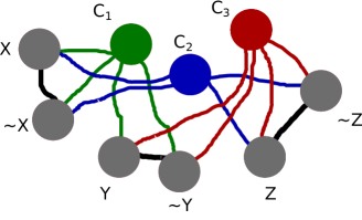
Figure 1: Neural oscillator model of the three random variable example. Here the three stimulus oscillators are represented by $C_{1}$, $C_{2}$, and $C_{3}$, and each stimulus is coupled to four response oscillators. Response oscillator $X$ corresponds to $\mathbf{X}=1$, ~$X$ to $\mathbf{X}=-1$, and so on.

It is easy to see how this oscillator model can produce the same correlations as the three random variables, by having each stimulus oscillator be a given context (not necessarily compatible with another oscillator’s context). We should emphasize that there are no matter-of-fact reasons for us to believe that, in the oscillator model, all three responses $\mathbf{X}$, $\mathbf{Y}$, and $\mathbf{Z}$ cannot be simultaneously computed. We could indeed imagine a behavioral experiment where contradictory responses from conditioned contexts could be elicited.

We now turn to quantum mechanics. To measure the correlations shown above, we need to pairwise measure each random variable. That means that $\mathbf{X}$, $\mathbf{Y}$, and $\mathbf{Z}$ pairwise commute. Thus, it is possible to find a basis in the Hilbert space where all corresponding quantum observables $\hat{X}$, $\hat{Y}$, and $\hat{Z}$ are diagonal, making it possible to measure $\mathbf{X}$, $\mathbf{Y}$, and $\mathbf{Z}$ simultaneously. Since we can measure then simultaneously, there must exists a joint probability distribution. Therefore, if a system is quantum mechanical, it cannot present correlations that are too strong as to not have a joint probability distribution, which rules out $-1$ or even $-1/3$.

The example shown illustrates an important point. In addition to non-Kolmogorovian probabilities, quantum mechanics brings a constraint on correlations encoded by the algebra of the Hilbert space. Furthermore, quantum dynamics requires more than just the assumption that physical states are described by vectors in a Hilbert space [33]. It should be emphasized that these constraints are quantum mechanical, and they do not apply to the oscillator model, and possibly not to the brain.

5 Conclusions

In this paper we discussed a contextual neural-oscillator brain model based on reasonable neurophysiological assumptions. We sketched how this neural-oscillator model could not only be used to obtain standard quantum-like features, such as a violation of Savage’s sure-thing principle, but also how it could be used to encode contextual random variables with no joint probability distribution. In fact, the oscillator-based system shown presents correlations that are so strong as to be incompatible with a Hilbert space representation of the corresponding observables.

We are then left with the question of how to better represent quantum-like dynamics in the brain, since Hilbert spaces seem too restrictive. Arguably, relaxing Kolmogorov’s axioms might be a feasible approach. For example, if we allow for the (unobservable) joint probabilities to be negative, we could use such values to compute correlations on unobserved situations (like the $\mathbf{X}$, $\mathbf{Y}$, and $\mathbf{Z}$ random variables) and test them against possible experimental conditions. So, we end with the following additional questions. Would the use of non-standard probabilities, perhaps guided by intuition from quantum mechanics, be a more appropriate tool to represent quantum-like effects in the social sciences than the use of vectors on Hilbert spaces? What type of formalism could at the same time give the required tools to represent contextual quantum-like dynamics without imposing the unnecessary constraints from a Hilbert space representation?

References

- Aerts [2009] Diederik Aerts. Quantum structure in cognition. Journal of Mathematical Psychology, 53(5):314–348, October 2009.
- Asano et al. [2010] Masanari Asano, Masanori Ohya, and Andrei Khrennikov. Quantum-Like model for decision making process in two players game. Foundations of Physics, 41(3):538–548, 2010.
- Bruza et al. [2009] Peter Bruza, Jerome R. Busemeyer, and Liane Gabora. Introduction to the special issue on quantum cognition. Journal of Mathematical Psychology, 53(5):303–305, 2009.
- Busemeyer et al. [2006] J. R. Busemeyer, Z. Wang, and J. T. Townsend. Quantum dynamics of human decision-making. Journal of Mathematical Psychology, 50:220–241, 2006.
- Busemeyer and Bruza [2012] Jerome R. Busemeyer and Peter D. Bruza. Quantum models of cognition and decision. Cambridge University Press, Cambridge, Great Britain, 2012.
- Busemeyer and Wang [2007] J.R. Busemeyer and Z. Wang. Quantum information processing explanation for interactions between inferences and decisions. In Proceedings of the Quantum Interaction Symposium AAAI Press, 2007.
- Busemeyer et al. [2009] J.R. Busemeyer, Z. Wang, and A. Lambert-Mogiliansky. Empirical comparison of markov and quantum models of decision making. Journal of Mathematical Psychology, 53(5):423–433, 2009.
- de Barros [2012] J. Acacio de Barros. Quantum-like model of behavioral response computation using neural oscillators. arXiv:1207.0033, 2012.
- de Barros and Suppes [2000] J. Acacio de Barros and P. Suppes. Inequalities for dealing with detector inefficiencies in Greenberger-Horne-Zeilinger type experiments. Physical Review Letters, 84:793–797, 2000.
- de Barros and Suppes [2001] J. Acacio de Barros and P. Suppes. Probabilistic results for six detectors in a three-particle GHZ experiment. In Jean Bricmont, D. Dürr, Maria Carla Galavotti, G. Ghirardi, F. Petruccione, and N. Zanghi, editors, Chance in Physics, volume 574 of Lectures Notes in Physics, page 213, 2001.
- de Barros and Suppes [2009] J. Acacio de Barros and P. Suppes. Quantum mechanics, interference, and the brain. Journal of Mathematical Psychology, 53(5):306–313, 2009.
- de Barros and Suppes [2010] J. Acacio de Barros and P. Suppes. Probabilistic inequalities and upper probabilities in quantum mechanical entanglement. Manuscrito, 33:55–71, 2010.
- Haven [2002] E. Haven. A discussion on embedding the Black–Scholes option pricing model in a quantum physics setting. Physica A: Statistical Mechanics and its Applications, 304(3–4):507–524, February 2002.
- Haven [2003] E. Haven. A Black-Scholes schrödinger option price: ‘bit’versus ‘qubit’. Physica A: Statistical Mechanics and its Applications, 324(1):201–206, 2003.
- Haven [2004] E. Haven. The wave-equivalent of the Black–Scholes option price: an interpretation. Physica A: Statistical Mechanics and its Applications, 344(1–2):142–145, December 2004.
- Haven [2005] E. Haven. Pilot-wave theory and financial option pricing. International Journal of Theoretical Physics, 44(11):1957–1962, 2005.
- Izhikevich [2007] Eugene M. Izhikevich. Dynamical Systems in Neuroscience: The Geometry of Excitability and Bursting. The MIT Press, Cambridge, Massachusetts, 2007.
- Jaynes [2003] E. T Jaynes. Probability theory: the logic of science. Cambridge Univ Pr, 2003.
- Khrennikov [2007a] A. Khrennikov. Bell’s inequality: Physics meets probability. arXiv:0709.3909, 2007a.
- Khrennikov [2007b] A. Khrennikov. Quantum-like description of probabilistic data from Shafir-Tversky experiments: evidence of trigonometric and hyperbolic (!) interference. arXiv:0708.2993v2, pages 1–25, 2007b.
- Khrennikov [2009a] A. Khrennikov. Can fluctuations of classical random field produce quantum averages? In Proceedings of SPIE, volume 7421, page 742102, 2009a.
- Khrennikov [2009b] A. Khrennikov. Quantum-like model of cognitive decision making and information processing. Biosystems, 95(3):179–187, 2009b.
- Khrennikov and Haven [2007] A. Khrennikov and E. Haven. The importance of probability interference in social science: rationale and experiment. arXiv:0709.2802v1, 2007.
- Khrennikov and Haven [2009] A. Khrennikov and E. Haven. Quantum mechanics and violations of the sure-thing principle: The use of probability interference and other concepts. Journal of Mathematical Psychology, 53(5):378–388, October 2009.
- Khrennikov [2010] Andrei Khrennikov. Ubiquitous Quantum Structure. Springer Verlag, Heidelberg, 2010.
- Khrennikova et al. [2012] Polina Khrennikova, Andrei Khrennikov, and Emmanuel Haven. The quantum-like description of the dynamics of party governance in the US political system. arXiv:1206.2888, June 2012.
- Kochen and Specker [1975] S. Kochen and E. P. Specker. The problem of hidden variables in quantum mechanics. In Clifford Alan Hooker, editor, The Logico-Algebraic Approach to Quantum Mechanics, page 293–328. D. Reidel Publishing Co., Dordrecht, Holland, 1975.
- Pais [1986] A. Pais. Inward bound: of matter and forces in the physical world. Oxford University Press, Oxford, UK, 1986.
- Penrose [1989] R. Penrose. Emperor’s New Mind. Oxford University Press, New York, 1989.
- Pothos and Busemeyer [2009] E. M Pothos and J. R Busemeyer. A quantum probability explanation for violations of ‘rational’decision theory. Proceedings of the Royal Society B: Biological Sciences, 276(1665):2171–2178, 2009.
- Robinson [2012] P. A. Robinson. Interrelating anatomical, effective, and functional brain connectivity using propagators and neural field theory. Physical Review E, 85(1):011912, January 2012. doi: 10.1103/PhysRevE.85.011912.
- Savage [1972] L. J Savage. The foundations of statistics. Dover Publications Inc., Mineola, New York, 2nd edition, 1972.
- Simon et al. [2001] Christoph Simon, Vladimír Bužek, and Nicolas Gisin. No-Signaling condition and quantum dynamics. Physical Review Letters, 87(17):170405, October 2001.
- Suppes and de Barros [1994a] P. Suppes and J. Acacio de Barros. A random-walk approach to interference. International Journal of Theoretical Physics, 33(1):179–189, 1994a.
- Suppes and de Barros [1996] P. Suppes and J. Acacio de Barros. Photons, billiards and chaos. In Paul Weingartner and Gerhard Schurz, editors, Law and Prediction in the Light of Chaos Research, volume 473, pages 189–201. Springer Berlin Heidelberg, 1996.
- Suppes and de Barros [2007] P. Suppes and J. Acacio de Barros. Quantum mechanics and the brain. In Quantum Interaction: Papers from the AAAI Spring Symposium, Technical Report SS-07-08, page 75–82, Menlo Park, CA, 2007. AAAI Press.
- Suppes et al. [2012] P. Suppes, J. Acacio de Barros, and G. Oas. Phase-oscillator computations as neural models of stimulus–response conditioning and response selection. Journal of Mathematical Psychology, 56(2):95–117, April 2012.
- Suppes and de Barros [1994b] Patrick Suppes and J. Acacio de Barros. Diffraction with well-defined photon trajectories: A foundational analysis. Foundations of Physics Letters, 7(6):501–514, December 1994b.
- Suppes and Zanotti [1981] Patrick Suppes and Mario Zanotti. When are probabilistic explanations possible? Synthese, 48(2):191–199, 1981.
- Suppes et al. [1996a] Patrick Suppes, J. Acacio de Barros, and Gary Oas. A collection of probabilistic Hidden-Variable theorems and counterexamples. In Riccardo Pratesi and L. Ronchi, editors, Waves, Information, and Foundations of Physics: a tribute to Giuliano Toraldo di Francia on his 80th birthday, Florence, Italy, October 1996a. Italian Physical Society. URL http://arxiv.org/abs/quant-ph/9610010.
- Suppes et al. [1996b] Patrick Suppes, J. Acacio de Barros, and Adonai S Sant’Anna. A proposed experiment showing that classical fields can violate bell’s inequalities. arXiv:quant-ph/9606019, June 1996b.
- Suppes et al. [1996c] Patrick Suppes, J. Acacio de Barros, and Adonai S. Sant’Anna. Violation of bell’s inequalities with a local theory of photons. Foundations of Physics Letters, 9(6):551–560, December 1996c.
- Suppes et al. [1996d] Patrick Suppes, Adonai Sant’Anna, and J. Barros. A particle theory of the casimir effect. Foundations of Physics Letters, 9(3):213–223, 1996d. ISSN 0894-9875. doi: 10.1007/BF02186404.
- Tversky and Shafir [1992] Amos Tversky and Eldar Shafir. The disjunction effect in choice under uncertainty. Psychological Science, 3(5):305–309, September 1992.
- Vassilieva et al. [2011] E. Vassilieva, G. Pinto, J. Acacio de Barros, and P. Suppes. Learning pattern recognition through Quasi-Synchronization of phase oscillators. IEEE Transactions on Neural Networks, 22(1):84–95, January 2011.
- Werndl [2009] C. Werndl. Are deterministic descriptions and indeterministic descriptions observationally equivalent? Studies in history and philosophy of science part B: studies in history and philosophy of modern physics, 40(3):232–242, 2009.