A critical analysis of the theoretical scheme to evaluate photoelectron spectra

Abstract

We discuss in depth the validity and limitations of a theoretical scheme to evaluate photo-electron spectra (PES) through collecting the phase oscillations at a given measuring point. Problems appear if the laser pulse is still active when the first bunches of outgoing flow reach the measuring point. This limits the simple scheme for evaluation of PES to low and moderate laser intensities. Using a model of free particle plus dipole field, we develop a generalized scheme which is shown to considerably improve the results for high intensities.

I Introduction

Photo-electron spectra (PES) constitute a longstanding basic tool for analyzing the electronic structure of atoms, molecules, or solids Turner and Jobory (1962); Turner (1970); Ghosh (1983). In the one-photon regime, PES provide an image of the sequence of single-particle levels which are occupied in the ground state. This has been applied, e.g., already in the early days of cluster physics to the electronic structure of cluster anions to track the transition to bulk metal McHugh et al. (1989). While this could be done with photon frequencies in the range of visible light, the analysis of deeper levels requires higher frequencies, and hence one finds also UV Rabalais (1977) and X-ray PES Moulder et al. (1962). Nowadays, we dispose of a great variety of coherent light sources in large ranges of frequency, intensity and pulse length, such as the very powerful and versatile free electron lasers Geloni et al. (2010); Bressler and Chergui (2010) which now even allow for time-resolved studies of deep lying core states of atoms embedded in a material Pietzsch et al. (2008). With the great availability of good light sources, studies of PES are now found in all areas of molecular physics, from atoms over simple molecules Tjeng et al. (1990) to complex systems as clusters Hoffmann et al. (2001) and organic molecules Liu and Hamers (1998).
There is hence a general need for a robust theoretical tool of analysis of PES in various dynamical regimes. Traditional approaches to compute PES rely on (multi-)photon perturbation theory Faisal (1987). A few years ago, we have developed a technique to evaluate the PES directly from numerical simulations of the electronic excitations on a spatial grid representation (and also for a plane-wave representation) Pohl et al. (2000, 2001) allowing exploration of a rather wide range of dynamical scenarios Pohl et al. (2000). The basic idea of the procedure is to use absorbing boundary conditions and to assume free particle propagation near the boundaries. The technique has indeed been successfully applied to a variety of clusters Reinhard and Suraud (2003); Fennel et al. (2010), for which significant electron emission can be achieved with comparatively low laser intensities. Atoms and molecules with larger ionization potentials (IP), as e.g. carbon, require stronger fields instead and it was found in first tests that the application of the recipe from Ref. Pohl et al. (2000) can yield artefacts for the case of long pulses with high intensity. Therefore it is a timely task to re-inspect the method and to develop improvements where found necessary. Such a critical analysis of the evaluation of PES on a numerical grid is the aim of this paper.

We start in section II with a brief review of the traditional recipe to evaluate PES. We show that, while this simple recipe works well for low laser intensities, it produces unphysical spectral features at high intensities, which call for a revision of the method. We continue with a quick reminder of the gauge freedom in describing the laser field. We discuss two choices of gauge and explain the gauge transformation that connects the two choices. The question which gauge is ideally to be used in the evaluation of PES will be answered in the course of the further sections. Afterwards, the presence of a strong laser field in coexistence with the emitted electrons is dealt with by solving the time-dependent Schrödinger equation for free electrons plus a homogeneous laser field. This case still allows closed solutions which is then used as a basic ingredient to define a refined recipe to evaluate PES. In section III, the refined recipe is then tested for the analytically solvable case of Gaussian wave packets first and then numerically for a few realistic test cases.

II Theoretical evaluation of PES

In this section, we first give a brief review of the scheme for the evaluation of PES introduced in Pohl et al. (2000, 2001). After showing that it is not appropriate for high laser intensities, we propose a generalized scheme that solves the problem. All schemes discussed here and in the previous papers rely on a mean-field description where each electron is associated with a single-electron wave function $\psi_{\alpha}$. We will consider in the formal discussions one representative state and drop the index $\alpha$ to simplify notations.

II.1 PES scheme for free electron

The PES are calculated in a very efficient manner exploiting the features of the absorbing boundary conditions Pohl et al. (2000, 2001). We give here a brief summary of the procedure and its motivation, first for the simple case of 1D and then in 3D. It is to be noted that these traditional recipes for evaluating the PES are deduced under the assumption of free particle propagation near the bounds of the numerical box.

II.1.1 The 1D case

We choose a “measuring point” $z_{\mathcal{M}}$ far away from the center and one or two grid points before the absorbing boundaries. We record the wave function $\psi(z,t)$ at the measuring point $z_{\mathcal{M}}$ during the time evolution. This delivers the raw information from which we extract the PES. In order to develop an appropriate recipe, we now need a few formal considerations.

We assume that the mean-field is negligible at $z_{\mathcal{M}}$ such that we encounter there free particle dynamics which is governed by the one-particle time-dependent Schrödinger equation $\mathrm{i}\partial_{t}\psi(z,t)=-\frac{\nabla^{2}}{2}\psi(z,t)$. The solution is

$$\psi(z,t)=\int\frac{\ \mathrm{d}k}{\sqrt{2\pi}}\,g(k)\,e^{\mathrm{i}(kz-\omega t)}$$ (1)

with the condition that $k$ and $\omega$ satisfy the dispersion relation $\omega=k^{2}/2$. Note that atomic units ($\hbar=m_{e}=e=4\pi\epsilon_{0}=1$) are used here and throughout the paper. The measurement of PES is practically a momentum analysis of the outgoing wave packet at a remote side. In momentum space, the wave function (1) reads

$$\widehat{\psi}(k,t)=\int\frac{dz}{\sqrt{2\pi}}e^{-\mathrm{i}kx}\psi(z,t)=\underbrace{\widehat{\psi}(k,0)}_{\propto g(k)}e^{-\mathrm{i}\omega t}\quad.$$ (2)

The probability to find an outgoing particle with momentum $k$ is thus given by $|\widehat{\psi}(k,t)|^{2}=|\widehat{\psi}(k,0)|^{2}$, from which the PES can be obtained as

$$\mathcal{Y}(E_{\mathrm{kin}})\propto\frac{1}{\sqrt{E_{\mathrm{kin}}}}\left|\widehat{\psi}(k,0)\right|^{2}\quad,$$ (3)

where $E_{\mathrm{kin}}=k^{2}/2=\omega$ is the kinetic energy and we have taken into account the appropriate energy density $\propto E^{-1/2}_{kin}$. This is what we call in this work the exact definition of PES developed close to the experimental procedure.

However, it is numerically extremely expensive to evaluate the PES by Fourier transformation for a remote slot in coordinate space. To overcome this difficulty, we obtain the expansion coefficient $g(k)$ from the Fourier transform in time-frequency space of the wave function $\psi(z,t)$ collected at a measuring point $z_{\mathcal{M}}$ near the absorbing boundary. We denote the Fourier transformation in time by $\widetilde{\psi}$ to distinguish it from the spatial Fourier transform $\widehat{\psi}$. This then reads :

$$\widetilde{\psi}(z_{\mathcal{M}},\omega^{\prime}) = \int\frac{\ \mathrm{d}t}{\sqrt{2\pi}}\,\psi(z_{\mathcal{M}},t)\,e^{\mathrm{i}\omega^{\prime}t}$$ (4)

$$= \int\frac{\ \mathrm{d}t}{\sqrt{2\pi}}\int\frac{\ \mathrm{d}k}{\sqrt{2\pi}}\,g(k)\,e^{\mathrm{i}(kz_{\mathcal{M}}-\omega t)}e^{i\omega^{\prime}t}$$ (5)

$$= \int\frac{\mathrm{d}k}{\sqrt{2\pi}}\,g(k)\,e^{\mathrm{i}kz_{\mathcal{M}}}\delta(\omega-\omega^{\prime})\ .$$ (6)

Since we collect $\psi(z_{\mathcal{M}},t)$ far away from the center and close to the absorbing boundary, we can assume that only outgoing waves will pass the measuring point $z_{\mathcal{M}}$. We will hence have only positive wave vectors

$$\omega=\frac{k^{2}}{2}\quad\longleftrightarrow\quad k=+\sqrt{2\omega}\quad,$$ (7)

which allows us to approximate the last line in (6) as

$$\widetilde{\psi}(z_{\mathcal{M}},\omega^{\prime}) \simeq \int_{0}^{\infty}\frac{\ \mathrm{d}\omega}{\sqrt{4\pi\omega}}\,g(\omega)\,e^{i\,z_{\mathcal{M}}\sqrt{2\omega}}\,\delta(\omega-\omega^{\prime})$$ (8)

$$= \frac{g(\omega^{\prime})}{\sqrt{4\pi\omega^{\prime}}}e^{i\,z_{\mathcal{M}}\sqrt{2\omega^{\prime}}}\ \theta(\omega^{\prime})\ .$$ (9)

In the last line, $\theta$ stands for the Heaviside function. Using (9) and (6), we finally obtain

$$g(\omega)\simeq\sqrt{4\pi\omega}\,e^{-\mathrm{i}\,z_{\mathcal{M}}\sqrt{2\omega}}\ \widetilde{\psi}(z,\omega)\ ,$$ (10)

where from now on, we will always consider $\omega>0$ and thus omit the factor $\theta(\omega)$ in Eq. (10). At measuring point $z_{\mathcal{M}}$, we can identify $\widetilde{\psi}(z_{\mathcal{M}},\omega)$ with $\widetilde{\psi}(z_{\mathcal{M}},E_{\rm kin})$ where $E_{\rm kin}$ is the kinetic energy of the electron. This defines the PES yield $\mathcal{Y}_{z_{\mathcal{M}}}(E_{\rm kin})$ as

$$\mathcal{Y}_{z_{\mathcal{M}}}(E_{\rm kin})\propto\sqrt{E_{\rm kin}}\left|\widetilde{\psi}(z_{\mathcal{M}},E_{\rm kin})\right|^{2}\ .$$ (11)

We have checked the method in extensive 1D wave packet calculations and compared it to a direct momentum decomposition of the outgoing wave as given in Eq. (3). Both methods yield the same results, while the above sketched frequency analysis at a ”measuring point” is orders of magnitude faster.

II.1.2 The 3D case

As in 1D, we assume for the 3D case free propagation and purely outgoing waves at the measuring point $\mathbf{r}_{\mathcal{M}}$. The solution of the one-particle time-dependent Schrödinger equation in free space reads

$$\psi(\mathbf{r},t)=\int\frac{\ \mathrm{d}^{3}\mathbf{k}}{\sqrt{(2\pi)^{3}}}\,g(\mathbf{k})\,e^{i(\mathbf{k}\cdot\mathbf{r}-\omega t)}\quad.$$ (12)

Analogously as in Eq. (7) for the 1D case, we calculate the coefficients $g(\mathbf{k})$ from the time Fourier transform of $\psi(\mathbf{r},t)$, assuming that only wave vectors $\mathbf{k}=k\,\mathbf{e}_{\mathbf{r}}$ with $k>0$ contribute, where $\mathbf{e}_{\mathbf{r}}$ is the direction of the outgoing radial wave. This yields

$$g(\omega,\Omega_{\mathbf{r}})\propto\,\widetilde{\psi}(\mathbf{r},\omega)\ ,$$ (13)

where $\Omega_{\mathbf{r}}$ is the solid angle related to the $\mathbf{r}$ direction. Considering $\mathbf{r}_{\mathcal{M}}$ as the measuring point, we compute the PES in direction $\Omega_{\mathbf{r}_{\mathcal{M}}}$ as

$$\mathcal{Y}_{\Omega_{\mathbf{r}_{\mathcal{M}}}}(E_{\rm kin})\,\propto\,\left|\widetilde{\psi}(\mathbf{r}_{\mathcal{M}},E_{\rm kin})\right|^{2}\ .$$ (14)

The above analysis yields the fully energy- and angular-resolved PES. The angular averaged PES would then be attained by angular integration with proper solid angle weights. It has nevertheless to be emphasized that the resulting angular dependence in the laboratory frame depends on the orientation of the molecule (or cluster). Actual ensembles in the gas phase do not contain molecules in well defined orientation but represent rather an equi-distribution of all possible orientations. A typical example are the many recent measurements of angular-resolved PES in cluster physics see, e.g., Pinaré et al. (1999); Wills et al. (2004); Kostko et al. (2007); Bartels et al. (2009); Kjellberg et al. (2010). An appropriate orientation averaging has to be performed before one can compare $\mathcal{Y}_{\Omega_{\mathbf{r}_{\mathcal{M}}}}(E_{\rm kin})$ with experimental data. The practical procedures for that are outlined in Wopperer et al. (2010a, b). Orientation averaging, however, is beyond the scope of the present paper and will be ignored in the following.

II.1.3 Example of application and problem

Although this simple scheme has been applied with success to a variety of clusters, our recent attempts to compute the PES of small covalent molecules have raised some questions concerning its general applicability. For high laser intensities, we find an unexpected shoulder in the PES at large kinetic energies. These pattern were then also found for the simple test case of Na_n clusters with jellium background when going to sufficiently large laser field strengths. This excludes particularities of pseudo-potentials, local or non-local ones. The problem seems to reside in the scheme to evaluate PES.

Figure 1 demonstrates the problem for the case of Na${}_{9}^{+}$. The spherical jellium model is used for the ionic background. Valence electrons are described by the time-dependent local-density approximation (TDLDA) using the energy functional of Perdew and Wang (1992) and an average-density self-interaction correction (ADSIC) Legrand et al. (2002).

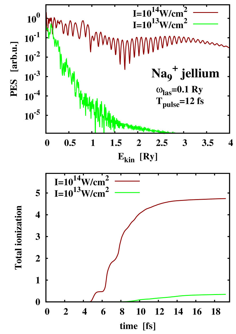
Figure 1: Ionization properties of Na${}_{9}^{+}$ with jellium background under the influence of laser pulses having frequency $\omega_{\mathrm{las}}=0.1$ Ry, pulse length $T_{\mathrm{pulse}}=12$ fs, and intensities $I=10^{13}$ W/cm² (green or light gray lines) and $I=10^{14}$ W/cm² (brown or dark gray lines), computed in a cylindrical box of 176$\times$88 $a_{0}^{2}$ with spherical absorbing bounds covering at least 16 grid points. The laser field was given effectively in $v$-gauge. Bottom : Time evolution of ionization. Left : Photoelectron spectra $\mathcal{Y}_{\Omega_{\mathbf{r}_{\mathcal{M}}}}(E_{\rm kin})$, see Eq. (14).

Two cases are considered for comparison: one with still moderate laser intensity, and another one in the high intensity regime. In the latter regime, more than half of the cluster’s electrons are stripped off, as shown in the bottom panel of Figure 1. The top panel shows the PES for both cases. For moderate intensity, we see the typical monotonous decrease. The case of high intensity differs : Up to $E_{\mathrm{kin}}\approx 1.5$ Ry, we see the typical pattern of a monotonous decrease of the envelope with some fluctuations. For $E_{\mathrm{kin}}>1.8$ Ry, however, we observe a new maximum, a broad shoulder of high energy electrons; this is totally unexpected and most probably unphysical. In the following, we clarify the origin of such a shoulder and we generalize the method to compute PES to a wider range of laser intensities.

II.2 Space gauge and velocity gauge

Before proceeding with a cure for the PES scheme illustrated above, we review the choices of gauge for describing the laser field. The external laser field is described in the limit of long wave lengths and neglecting magnetic effects (electronic velocities are very small at any time). The electron-laser interaction can be described either by a time-dependent scalar potential $\Phi(\mathbf{r},t)$ or a time-dependent vector potential $\mathbf{A}(\mathbf{r},t)$ in the Hamiltonian, which in general reads

$$H(\mathbf{r},t)=\frac{1}{2}\left[\hat{\mathbf{p}}+\frac{{\mathbf{A}}(\mathbf{r},t)}{c}\right]^{2}-\Phi(\mathbf{r},t)\ .$$ (15)

In the space gauge ($x$-gauge), the laser field is described, within the dipole approximation, by a scalar potential only:

$${\mathbf{A}}^{(x)}(\mathbf{r},t)=\mathbf{0},\qquad\Phi^{(x)}(\mathbf{r},t)=-E_{0}f(t){z}\ ,$$ (16a)

where the laser polarization is chosen along the $$z E_{0} f(t)$$ axis, and is the maximum electric field of the laser. here denotes the temporal profile of the laser pulse, taken as:

$$f(t)=\sin(\omega_{\mathrm{las}}^{\mbox{}}t)\sin^{2}\!\left(\!\frac{\pi\,t}{T_{\mathrm{pulse}}}^{\mbox{}}\!\right)\theta(t)\ \theta(T_{\mathrm{pulse}}^{\mbox{}}\!-\!t)\ ,$$ (16b)

where $\omega_{\mathrm{las}}$ and $T_{\rm pulse}$ are respectively the frequency and the duration of the laser pulse. $\theta$ denotes the Heaviside function. We have chosen a smooth $\sin^{2}$ profile which combines high spectral selectivity and finite extension. The spectral selectivity is needed because the pulse profile carries through to the PES Pohl et al. (2001).

In the velocity gauge ($v$-gauge) instead, the laser field enters the Hamiltonian as a vector potential only:

$${\mathbf{A}}^{(v)}(\mathbf{r},t)=-cE_{0}F(t)\,\mathbf{e}_{z}\ ,\quad\Phi^{(v)}(\mathbf{r},t)=0\ ,$$ (17a)

with

$$F(t)=\int^{t}_{-\infty}\mathrm{d}t^{\prime}\,f(t^{\prime}).$$ (17b)

Note that the vector potential in dipole approximation is spatially constant.

Both gauges are equivalent. They are connected by a gauge transformation which in general reads :

$$\Phi^{\prime} = \Phi+\frac{\dot{\chi}}{c}\quad,$$ (18a)

$$\mathbf{A}^{\prime} = \mathbf{A}-\nabla{\chi}\quad,$$ (18b)

$$\psi^{\prime} = \psi\,\exp{\left(\frac{i\chi}{c}\right)}\quad.$$ (18c)

Let us assume that we take the $v$-gauge as a starting point : the laser field is described by the vector potential $\mathbf{A}^{(v)}=-cE_{0}F(t)\mathbf{e}_{z}$, whereas $\Phi^{(v)}=0$. If we want to gauge transform the vector potential into the scalar potential, then $\nabla\chi=\mathbf{A}^{(v)}$, from where

$$\chi=-cE_{0}F(t)z\quad\Rightarrow\quad\Phi^{(x)}=\frac{\dot{\chi}}{c}=-E_{0}f(t)z\ .$$ (19)

This finally gives

$$\psi^{(x)}=\psi^{(v)}\exp{\left[-iE_{0}F(t)z\right]}\,$$ (20)

which relates the wave function $\psi^{(x)}$ as computed by time propagation under the action of the scalar potential (16a), and $\psi^{(v)}$ for the case with the vector potential (17). It is obvious that this phase factor is crucial in the present PES analysis, while it can easily be ignored for local observables as, e.g., dipole momentum or net ionization.

The phase transformation allows one to decouple the gauge used in the analysis from that used in the time evolution. Assume that we solve the Schrödinger equation using the potentials (17). This immediately yields the wave function $\psi^{(v)}$ in $v$-gauge. The same wave function could be obtained by using (16) and applying the reverse transformation (20) to recover $\psi^{(v)}$ from the $\psi^{(x)}$ as obtained by propagation. In fact, this is the most efficient way to evaluate $\psi^{(v)}$ as the operator (16a) is purely local. It is to be noted that the transformation (20) is relevant for the PES only if the outgoing wave reaches the measuring point $z_{\mathcal{M}}$ at a time where the signal $F(t)$ is still active. For very large boxes, the outgoing wave and the signal can avoid to coincide, in which case each gauge yields the same result. However, typical box sizes used in practice are not always that large.

The question is now which gauge is most suitable for evaluating PES. The basic papers Pohl et al. (2000); Pohl (2003) state that the preferable choice is the $v$-gauge. The argument there was a better convergence with box size. We now speculate that this has to do with (non-)coincidence of outgoing wave packet and laser signal. In the next section, this will be scrutinized using a solvable model.

II.3 PES scheme for free particles plus laser field

In section II, we have deduced the recipe for evaluating PES under the assumption that the potential is negligible at the measuring point. Although this may hold for the typical mean field of a system, we cannot easily exclude the presence of the laser field at this point because the laser field is of extremely long range (wave length much larger than system size in the dipole approximation that we use here). Thus we extend the considerations to the case of a free particle plus laser field in dipole approximation which is still analytically solvable. We confine the considerations to the 1D case. The extension to 3D is straightforward.

II.3.1 Momentum-space wave function in $v$-gauge

We first consider the Schrödinger equation of a free particle with the external field (17) in $v$-gauge

$$\frac{1}{2}\big{[}\hat{\mathbf{p}}-E_{0}F(t)\,\mathbf{e}_{z}\big{]}^{2}\psi^{(v)}(z,t) = \mathrm{i}\,\partial_{t}\psi^{(v)}(z,t)\quad,$$ (21a)

$$\psi^{(v)}(z,0) = \psi^{(v)}_{0}(z)\quad.$$ (21b)

It is advantageous to expand the wave function at a given time in momentum space:

$$\psi^{(v)}(k,t) = \int\frac{\ \textrm{d}z}{\sqrt{2\pi}}\,e^{-\mathrm{i}kz}\,\widehat{\psi}^{(v)}(z,t)\ ,$$ (22a)

$$\widehat{\psi}^{(v)}(k,0) = \widehat{\psi}^{(v)}_{0}(k)\ .$$ (22b)

This yields the Schrödinger equation in the form

$$\frac{1}{2}\big{[}k-E_{0}F(t)\big{]}^{2}\,\widehat{\psi}^{(v)}(k,t)=\mathrm{i}\,\partial_{t}\widehat{\psi}^{(v)}(k,t)\ ,$$ (23)

which solution reads :

$$\widehat{\psi}^{(v)}(k,t)=\exp{\left(-\frac{\mathrm{i}}{2}\int_{0}^{t}\mathrm{d}t^{\prime}\,\big{[}k-E_{0}F(t^{\prime})\big{]}^{2}\right)}\widehat{\psi}^{(v)}_{0}(k)\ .$$ (24)

We rewrite the latter expression as

$$\widehat{\psi}^{(v)}(k,t)=\exp{\big{(}-\mathrm{i}\omega t+\mathrm{i}k\delta q-\mathrm{i}\delta\Omega\big{)}}\,\widehat{\psi}^{(v)}_{0}(k)$$ (25a)

with

$$\omega = \frac{k^{2}}{2}\quad,$$ (25b)

$$\delta q(t) = E_{0}\int_{0}^{t}\mathrm{d}t^{\prime}\,F(t^{\prime})\quad,$$ (25c)

$$\delta\Omega(t) = \frac{E_{0}^{2}}{2}\int_{0}^{t}\mathrm{d}t^{\prime}\,F(t^{\prime})^{2}\quad.$$ (25d)

Eqs. (25) constitute the solution when propagating the wave packet in $v$-gauge.

II.3.2 Momentum-space wave function in $x$-gauge

The Schrödinger equation of the same situation in $x$-gauge reads

$$\left[\frac{\hat{\mathbf{p}}^{2}}{2}\,+\,E_{0}zf(t)\right]\,\psi^{(x)}(z,t) = \mathrm{i}\,\partial_{t}\psi^{(x)}(z,t)\quad,$$ (26a)

$$\psi^{(x)}(z,0) = \psi^{(x)}_{0}(z)\quad,$$ (26b)

$$f = \partial_{t}F\quad.$$ (26c)

Note that at $t=0$, the laser field is off and therefore, the wave function in $x$-gauge is the same as that in $v$-gauge. In the following, we hence indicate the wave function in $k$ space at $t=0$ indifferently as $\widehat{\psi_{0}}(k)$ since the upper script $(x)$ or $(v)$ is irrelevant. Thanks to the gauge transformation (20), the solution of (26a) can be easily obtained from the solution (25a) in $v$-gauge, that is :

$$\widehat{\psi}^{(x)}(k,t)=\widehat{\psi}^{(v)}\left(k+E_{0}F(t),t\right)\quad.$$ (27)

The wave function in $x$-gauge thus becomes

$$\widehat{\psi}^{(x)}(k,t)=\exp{\left(-\mathrm{i}\omega t+\mathrm{i}K\delta q-\mathrm{i}\delta\Omega\right)}\ \widehat{\psi}_{0}(k),$$ (28a)

with

$$K = k+E_{0}F(t)\quad,$$ (28b)

$$\omega = \frac{K^{2}}{2}\quad,$$ (28c)

where $\delta q$ and $\delta\Omega$ as given in Eqs. (25c) and (25d) respectively. This form is considerably more involved than the solution (25a) in $v$-gauge, since $K$ explicitly depends on time $t$. We hence take this as a first formal indication that the preferred gauge to evaluate PES should be the $v$-gauge.

II.3.3 Reconstruction of the PES

The scheme to evaluate PES, as sketched in section II, collects a wave function at a certain coordinate-space point $z_{\mathcal{M}}$ and performs Fourier transformation in frequency. This yields, by virtue of $\omega=k^{2}/2$, the outgoing wave function in momentum space from which we then deduce the PES. In extension of the simple form (11), we now want to take care of the possible coincidence of the laser field at the measuring point with the by-passing outgoing wave. This setup has been solved in section II.3.1. We are now going to apply the PES analysis to the solution (25a) and deduce how to modify the collected signal at $z_{\mathcal{M}}$ in order to properly describe the underlying unperturbed wave packet $\widehat{\psi}_{0}(k)$.

The relation between the wave function in frequency space and that in momentum space is given by

$$\widetilde{\psi}(z,\omega) = \int\!\frac{\textrm{d}t}{\sqrt{2\pi}}\,e^{i\omega t}\psi(z,t)$$ (29)

$$= \int\frac{\textrm{d}k}{\sqrt{2\pi}}\,e^{ikz}\int\!\frac{\textrm{d}t}{\sqrt{2\pi}}\,e^{i\omega t}\widehat{\psi}(k,t)\ .$$ (30)

In the case where the laser field at the measuring point is negligible, one can see from Eqs. (25a) and (25b) that the solution in $k$-space shrinks to a simple $\widehat{\psi}^{(v)}(k,t)=\exp{\left(-i\omega^{\prime}t\right)}\,\widehat{\psi}_{0}(k)$ with $\omega^{\prime}=\frac{k^{2}}{2}$. Then the integration over $t$ in (30) immediately produces a $\delta(\omega-\omega^{\prime})$, and that over $k$, using the fact that $k=\sqrt{2\omega^{\prime}}$ close to the absorbing boundary, yields $\widetilde{\psi}^{(v)}(z,\omega)\propto\widehat{\psi}_{0}(k)$. Therefore, the PES in Eq. (3) can be directly evaluated from $\widetilde{\psi}(z,\omega)$ (see Eq. (11)).

Now we proceed to the case with non-vanishing laser field at the measuring point, once again in $v$-gauge. Trying to apply the time-frequency transformation directly to the $k$-space solution (25a) runs into trouble due to the non-trivial time dependences induced by the factors $\delta q(t)$ and $\delta\Omega(t)$. An obvious solution is simply to counter-weight the disturbing phase factors by a phase-correction factor $\exp{\left(-\mathrm{i}k\delta{q}+\mathrm{i}\delta\Omega\right)}$. This can be done even in coordinate space because these factors do not depend on the position. Therefore we calculate the PES from a phase-augmented Fourier transform $\widetilde{\psi}^{\mathrm{(PA)}}$, which is now proportional to

$$\widetilde{\psi}^{\mathrm{(PA)}}(z_{\mathcal{M}},\omega) \propto \int\textrm{d}t\,e^{\mathrm{i}\omega t}e^{\mathrm{i}\varphi}\psi^{(v)}(z_{\mathcal{M}},t)\quad,$$ (31a)

$$\varphi = -k\delta q+\delta\Omega\quad.$$ (31b)

This modified Fourier transform is then used as in Eqs. (11) yielding the recipe for the 1D case

$$\mathcal{Y}_{z_{\mathcal{M}}}(E_{\rm kin})\propto\sqrt{E_{\rm kin}}\left|\widetilde{\psi}^{\mathrm{(PA)}}(z_{\mathcal{M}},E_{\rm kin})\right|^{2}\ .$$ (32)

The generalization for the 3D case proceeds analogously.

The new move in this generalized evaluation is to augment the original recipe by the phase-correction factor $e^{\mathrm{i}\varphi}$. This should allow the application of the recipe in a wider range of laser intensities and time profiles. The factor becomes negligible for weak laser field, or for fields which do not interfere in time with the emitted particle flow. We shall call in the following the former recipe (11) the “raw” recipe and the generalized form (32) the “phase-augmented” (PA) recipe. A word of caution is in order. The additional phase involves the mere momentum $k$. The recipe (31a) identifies that with the frequency $\omega$ according to Eq. (7). This is just as valid as the Fourier transformation is selective in frequency. This may be at stake in cases of very violent dynamics.

We run into unsurmountable trouble if we try to develop a generalized scheme on the basis of the solution (28a) in $x$-gauge because here even the instantaneous momentum $K$, as given in Eq. (28b), depends on time. This is another strong indication that the $v$-gauge is the appropriate starting point for evaluating the PES (as was already argued in Pohl et al. (2000); Pohl (2003)). We will confirm this suspicion in the next section with a practical example.

III Illustration

In this section, we show how the generalized scheme (31a) performs. We first apply it to an exactly solvable model, and then to more realistic cases.

III.1 Analytical test case: Gaussian wave packets

As a first test case, we consider a Gaussian wave packet whose propagation can be analytically described, even in the presence of a (homogeneous) laser field. The analytical solution, carried forth to far distance and beyond the lifetime of the laser field, allows a direct evaluation of the PES by filtering the momentum components by Fourier transformation from coordinate to momentum space. This “direct” analysis exactly corresponds to the experimental procedure, see Eq. (3). Thus we can test the PES analysis in frequency space against these “exact” results.

III.1.1 Gaussian wave packet in a laser field

We consider a one dimensional system with a Hamiltonian consisting of the free kinetic energy plus the external laser field, as it was discussed in section II.3. The wave function of the system at initial time is taken as the following Gaussian function:

$$\psi(z,0)=\frac{1}{(\pi\mu_{0})^{1/4}}\;\exp{\left(\mathrm{i}p_{0}z-\frac{(z-q_{0})^{2}}{2\mu_{0}}-\mathrm{i}\Omega_{0}\right)}\ .$$ (33)

The Fourier transform in $k$ space of (33) reads

$$\widehat{\psi}_{0}(k)=\left(\frac{\mu_{0}}{\pi}\right)^{1/4}\,e^{\mathrm{i}q_{0}(p_{0}-k)-\mathrm{i}\Omega_{0}}\ \exp{\left(-\frac{\mu_{0}}{2}(k-p_{0})^{2}\right)}\ .$$ (34)

The solution of the time-dependent Schrödinger equation is detailed in Appendix A, using the $x$-gauge. It reads:

$$\psi^{(x)}(z,t) = \left(\frac{\mu_{0}}{\pi({\mu_{0}}^{2}+t^{2})}\right)^{1/4}e^{\mathrm{i}\left(p_{0}-E_{0}F(t)\right)z}$$ (36)

$$\exp{\left(-\frac{[z-q(t)]^{2}}{2(\mu_{0}+\mathrm{i}t)}-\mathrm{i}\Omega(t)\right)}\ ,$$

with

$$q(t) = q_{0}+p_{0}t-E_{0}\int_{0}^{t}\textrm{d}t^{\prime}\,F(t^{\prime})\ ,$$ (37)

$$\Omega(t) = \Omega_{0}+\frac{p_{0}^{2}}{2}t-p_{0}E_{0}\int_{0}^{t}\textrm{d}t^{\prime}\,F(t^{\prime})$$ (38)

$$\qquad+\frac{{E_{0}}^{2}}{2}\int_{0}^{t}\textrm{d}t^{\prime}F^{2}(t^{\prime})+\frac{1}{2}\mathrm{atan}\left(\frac{t}{\mu_{0}}\right)\ .$$

Using now the gauge transformation (20), the wave function in $v$-gauge becomes

$$\psi^{(v)}(z,t) = \left(\frac{\mu_{0}}{\pi({\mu_{0}}^{2}+t^{2})}\right)^{1/4}e^{\mathrm{i}p_{0}z}$$ (40)

$$\exp{\left(-\frac{[z-q(t)]^{2}}{2(\mu_{0}+\mathrm{i}t)}-\mathrm{i}\Omega(t)\right)}\ .$$

III.1.2 Exact evaluation of PES by spatial Fourier analysis

An exact evaluation of the PES has to analyze the momentum content of a wave packet at a place where free propagation is reached. The momentum distribution computed from the wave packet $\psi^{(x)}$ by spatial Fourier transformation becomes

$$\widehat{\psi}^{(x)}(k,t) = \left(\frac{\mu_{0}}{\pi}\right)^{1/4}e^{\mathrm{i}\arg(\mu)/2}\ \exp{\big{(}-\frac{\mu}{2}[k-p(t)]^{2}\big{)}}$$ (41)

$$\qquad\exp{\big{(}\mathrm{i}[p(t)-k]q(t)-\mathrm{i}\Omega(t)\big{)}}$$

where $\arg(\mu)$ denotes the argument of $\mu$. The momentum distribution and corresponding probability becomes in $v$-gauge

$$\widehat{\psi}^{(v)}(k,t) = \left(\frac{\mu_{0}}{\pi}\right)^{1/4}e^{\mathrm{i}\arg(\mu)/2}\ \exp{\left(-\frac{\mu}{2}[k-p_{0}]^{2}\right)}$$

$$\qquad\exp{\big{(}\mathrm{i}[p_{0}-k]q(t)-\mathrm{i}\Omega(t)\big{)}}\quad,$$

$$\left|\widehat{\psi}^{(v)}(k,t)\right|^{2} = \left(\frac{\mu_{0}}{\pi}\right)^{1/2}\exp{\left(-{\mu_{0}}[k-p_{0}]^{2}\right)}\quad.$$ (42)

The corresponding kinetic energy distribution is obtained by the identification $k=+\sqrt{2E_{\mathrm{kin}}}$. One also has to account for the appropriate energy density $\propto E_{\mathrm{kin}}^{-1/2}$. This yields

$$\mathcal{Y}^{(v)}(E_{\mathrm{kin}}) \propto \sqrt{\frac{1}{E_{\mathrm{kin}}}}\left|\widehat{\psi}^{(x)}(\sqrt{2E_{\mathrm{kin}}})\right|^{2}$$ (43)

$$= \sqrt{\frac{1}{E_{\mathrm{kin}}}}\left(\frac{\mu_{0}}{\pi}\right)^{1/2}e^{-{\mu_{0}}(\sqrt{2E_{\mathrm{kin}}}-p_{0})^{2}}$$

This is then the exact energy distribution evaluated from spatial Fourier transform.

III.1.3 Evaluation with the phase-augmented PES scheme

The final PES analysis for the above model relies on the wave functions at the measuring point, i.e. $\psi^{(x)}(z_{\mathcal{M}},t)$ and $\psi^{(v)}(z_{\mathcal{M}},t)$ as given in Eqs. (40) and (36), respectively. We use the laser profile (16b). As an actual example, we consider the following parameters: $p_{0}=1\,\mathrm{a}_{0}^{-1}$, $q_{0}=0$, $\Omega_{0}=0$, $\omega_{\mathrm{las}}=0.11\,\mathrm{Ry}=1.4\,\mathrm{eV}$, $T_{\mathrm{pulse}}=8000\,\mathrm{Ry}^{-1}=384\,\mathrm{fs}$, $\mu_{0}=100\,\mathrm{a}_{0}$ and various field strengths $E_{0}$. The measuring point was taken at $z_{\mathcal{M}}=1000\,\mathrm{a}_{0}$ or $2000\,\mathrm{a}_{0}$. The first choice yields an overlap between laser pulse and flow signal at $z_{\mathcal{M}}$ while the second choice decouples them. In the following discussion, we quantify the field strength in terms of the laser intensity. The correspondence is, e.g., $I=10^{14}$ W/cm${}^{2}\leftrightarrow E_{0}=0.109$ Ry/a₀, $I=10^{12}$ W/cm${}^{2}\leftrightarrow E_{0}=0.0109$ Ry/a₀, $I=10^{10}$ W/cm${}^{2}\leftrightarrow E_{0}=0.00109$ Ry/a₀.

Figure 2 compares the evaluation of PES for $x$-gauge versus $v$-gauge for a case of weak laser field where the phase correction $\mathcal{\varphi}$ in Eq. (31a) is negligible such that we can effectively use the “raw recipe” (11).

Figure 2: Photoelectron spectra from wave packet analysis for a weak intensity $I=10^{10}$ W/cm². We use the “raw” recipe (11) and compare analysis from the wave function in $v$- (brown or dark curve) and $x$-gauge (green or light gray line). The exact result, that is the momentum distribution of the wave packet as given in Eq. (43) is also shown (black line).

Laser pulse length, wave packet, and measuring point have been chosen such that the wave packet runs through the measuring point at a time where the laser is still fully active. It becomes obvious that the result from the wave function in $x$-gauge is unphysical. The source of the problem lies in the contribution $\exp{\left(ip(t)z_{\mathcal{M}}\right)}$. As soon as the momentum $p=p(t)$ moves even slightly, the possibly large $z_{\mathcal{M}}$ can amplify such a small oscillation and induce dramatic phase oscillations which, in turn, produce a large contribution to the PES. This contribution, however, must be unphysical because it sensitively depends on the choice of the measuring point. Clearly, the $v$-gauge is the preferred choice for the evaluation of PES. This was already expected from the analytical considerations in section II.3.3. We will henceforth exclusively use the $v$-gauge. Of course, a numerical solution of the Schrödinger equation in coordinate space is often much simpler in $x$-gauge. In such a case, one still can use the $x$-gauge for the solution and then use the gauge transformation (20) to bring this into $v$-gauge. This is the path actually followed in section III.2.

Results for higher intensities are collected in figure 3.

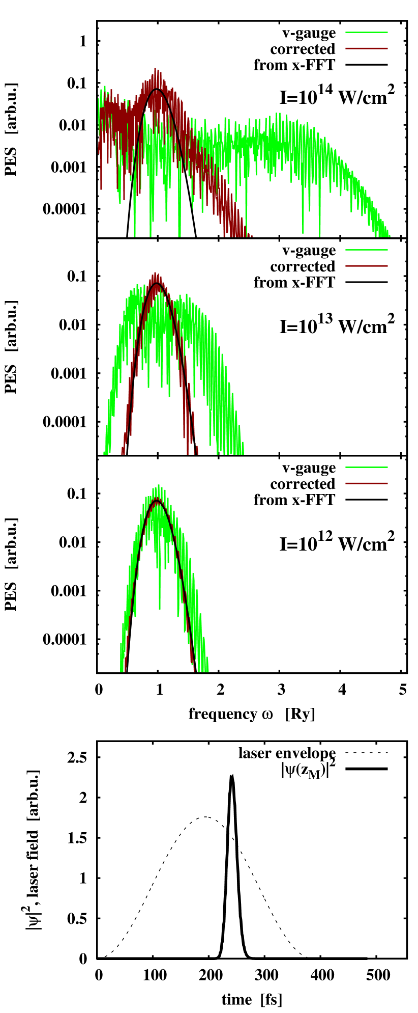
Figure 3: Photoelectron spectra from wave packet analysis. Lower panel: The laser pulse envelope (dashed line) and the probability density $|\psi(z_{\mathcal{M}},t)|^{2}$ at the measuring point (full line). Upper panels: PES analysis at $z_{\mathcal{M}}$ in $v$-gauge from “raw” (green or light gray curve) and with phase augmented (PA) signal (brown or dark gray line) for three laser intensities as indicated. For comparison, the momentum distribution of the wave packet as given in Eq. (43) is also shown (black curve).

Here we use $v$-gauge throughout and compare the “raw” recipe (11) with the PA recipe (31a). The lowest panel shows the laser profile (16b) together with the squared wave function $|\psi(z_{\mathcal{M}},t)|^{2}$ at the measuring point. This signals a critical situation where the laser is fully active while the wave packet is passing by the measuring point. The three upper panels show results for different intensities. The “raw” recipe still works acceptably well for the moderate intensity $I=10^{12}$ W/cm², but becomes grossly misleading for higher intensities. The generalized recipe (31a) visibly improves the performance. The results become reliable up to $I=10^{13}$ W/cm² and remain somehow qualitatively correct for the highest intensity. It is thus much preferably to use the phase augmented form (31a) for the evaluation of the PES.

Figure 4 shows results from a configuration where the measuring point has been moved farther away to $z_{\mathcal{M}}=2000$ which decouples the laser pulse from the wave packets signal.

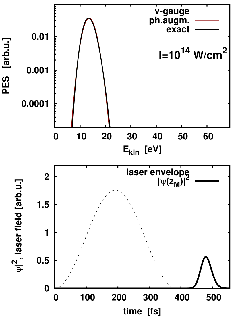
Figure 4: As in Figure 3 but for a situation where the laser pulse does not overlap with the wave packet at the measuring point (see bottom panel). Only the case of strongest laser intensity is shown.

The case of highest intensity $I=10^{14}$ W/cm² is shown. As expected, the “raw” recipe yields the same result as the PA one and both agree nicely with the exact result. Moreover, the $x$-gauge (not shown here) yields precisely the same result as the $v$-gauge. Thus all distinctions and considerations are unnecessary in the case that laser pulse and particle flow do not overlap.

III.2 Realistic test cases

As a first realistic test case, we come back to the introductory example of Figure 1, namely the cluster Na${}_{9}^{+}$ modeled with spherical jellium background and treated by time-dependent density functional theory using the energy functional of Perdew and Wang (1992). We take the laser with a typical infrared frequency and two rather large intensities. The axial symmetry of this and of the following example allows us to perform the calculations in cylindrical coordinates. Figure 5 shows the results for the “raw” and the PA recipes.

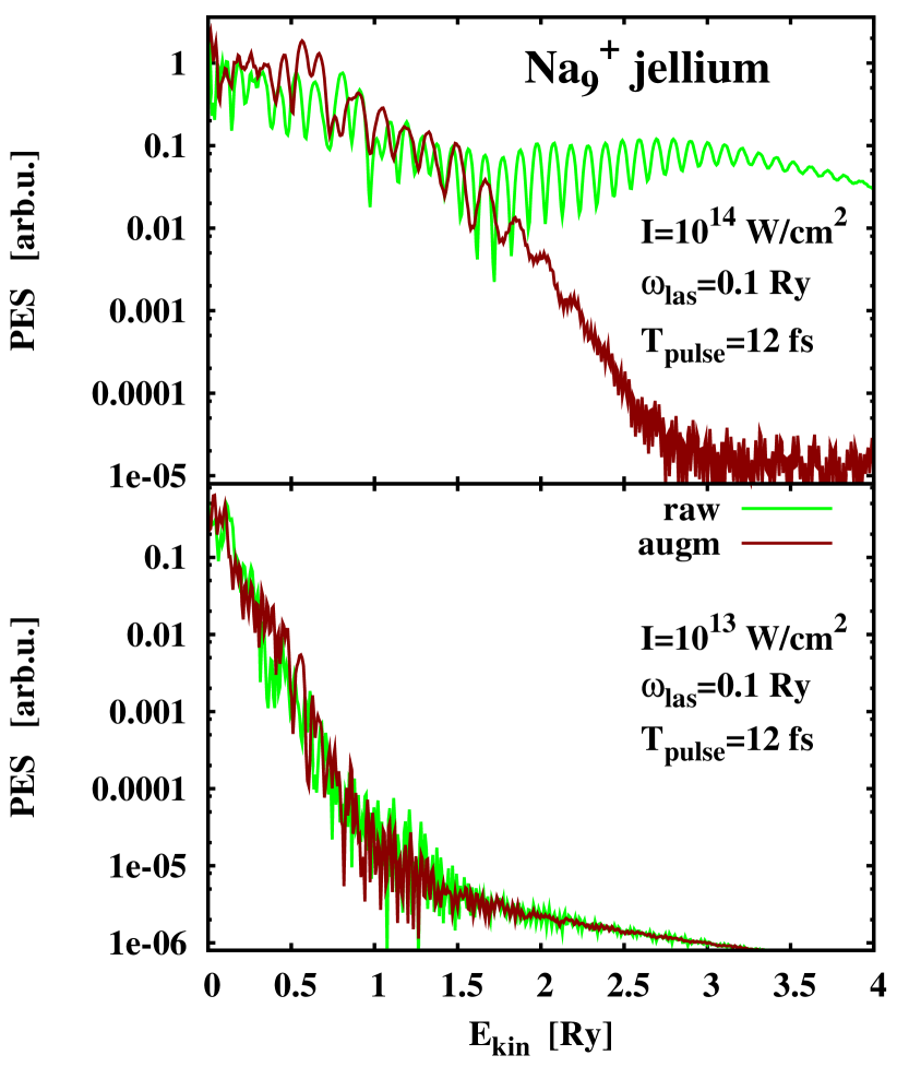
Figure 5: Ionization properties for Na${}_{9}^{+}$ with jellium background under the influence of a laser pulse having frequency $\omega_{\mathrm{las}}=0.1$ Ry, pulse length $T_{\mathrm{pulse}}=12$ fs, and intensity as indicated, computed in a cylindrical box of 176$\times$88 $a_{0}^{2}$ with spherical absorbing bounds covering at least 16 grid points. The laser field was given effectively in $v$-gauge. The “raw” results (green or light gray curves) are given by Eqs. (11), while the PA results (brown or dark gray curves) are complemented by the phase factor (31a).

The “raw” PES in the upper panel repeats the case of figure 5 showing the obnoxious high energy shoulder. The PA PES makes a dramatic difference. It shows a reasonable, almost monotonous, decrease of the envelope. Only at about 2.5 Ry, the decrease turns into a rather weak slope which may be unrealistic as we come here into a region of very low yield where unwanted background may spoil the analysis. The next lower intensity (lower panel) already shows reasonable pattern with the “raw” recipe. The PA recipe brings some improvement as it removes the glimpse of a shoulder at about 1.1 Ry. As already observed in the analytic case of a Gaussian wave packet, lower intensities perform well already with the “raw” recipe and the difference brought in from the PA recipe is negligible.

Figure 6 shows a next test case results for the C₄ chain, treated with non-local pseudo-potentials of Goedecker type Goedecker et al. (1996) and, again, the electronic energy-density functional of Perdew and Wang (1992).

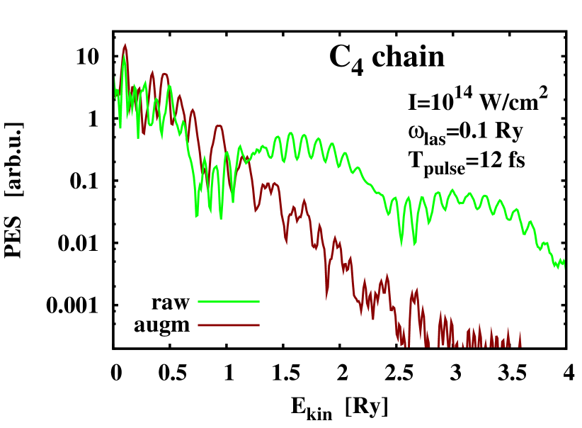
Figure 6: Ionization properties for the C₄ chain under the influence of a laser pulse having frequency $\omega_{\mathrm{las}}=0.1$ Ry, pulse length $T_{\mathrm{pulse}}=12$ fs, and intensity as indicated. The laser field was given effectively in $v$-gauge. The “raw” results (green of light gray curve) are given by Eqs. (11), while the PA results (brown or dark gray line) are complemented by the phase factor (31a).

The unphysical shoulders obtained with the “raw” recipe are even more developed than in case of Na${}_{9}^{+}$ and their successful removal by the PA recipe is impressive. This is a clear demonstration of the gain achieved by the PA recipe (31a).

IV Conclusion

We have investigated the evaluation of photo-electron spectra (PES) by sampling the time evolution of the wave function at a fixed measuring point. The schemes were first analyzed using solvable models. The traditional scheme was developed from the idea of a freely propagating outgoing wave. This requires negligible potentials at the measuring point which, in turn, sets a limit to an acceptable laser field strength. In order to extend the applicability of the scheme for evaluating PES to stronger fields, we have considered a model of a free particle plus an external laser field in dipole approximation. This model is still analytically solvable and the analytical solution allows us to deduce a more general scheme for the PES which consists in augmenting the collected wave function by an appropriate phase factor accounting for the time dependent laser field. We have also investigated the effect of gauge transformations on the results and pondered the question of the most appropriate choice of gauge. We have found that the appropriate gauge for evaluating PES is clearly the $v$-gauge (velocity gauge). Still, the most practical way to produce the wave functions in $v$-gauge is to compute them first in $x$-gauge (space gauge) and to apply then the appropriate gauge transformation.

The augmented scheme has been tested in an analytical model of Gaussian wave packets and in a few realistic examples. A major result is that the “raw” recipe for PES is valid for low and moderate laser fields (about $10^{12}$ W/cm² for the test case Na${}_{9}^{+}$). It remains valid in case that the particle flow arrives at the measuring point after the laser pulse has died out (in this case for all intensities). The phase augmented evaluation of PES was shown to considerably extend the range of applicability. The gain was particularly dramatic for the example of the C₄ chain. With the augmented recipe for computing PES we have been able to check laser intensities up to $10^{14}$ W/cm² for our realistic test cases which all involved a low laser frequency of 0.1 Ry. Higher laser frequencies reduce the effective intensity (Keldysh criterion). Thus even higher intensities may be used for higher frequencies.

After the successful tests shown here, the augmented recipe for evaluating PES is ready for use in more demanding situations as they are molecular systems with large ionization potentials for which experimental data already exist as, e.g., N₂, C₆₀ or typical organic molecules.

Appendix A Solution of the Schrödinger equation for the wave packet model

We provide the analytical solution of the wave packet propagation in $x$-gauge. This is simpler and the $v$-gauge is regained easily by the phase transformation (20).

The starting point is the Schrödinger equation as given in Eq. (21a). The ansatz for the solution is given by

$$\psi=\left(\frac{\mu_{0}}{\pi\,\mu^{*}(t)\mu(t)}\right)^{1/4}\;\exp{\!\left(ip(t)z\!-\!\frac{(z\!-\!q(t))^{2}}{2\mu(t)}-i\Omega(t)\!\right)}$$ (44)

with $\mu(t)=\mu_{0}+i\xi t$. The other time-dependent parameters are determined substituting (44) in the time-dependent Schrödinger equation and comparing term by term. In order to achieve this we first build the necessary derivatives:

$$\frac{\mathrm{i}\partial_{t}\psi}{\psi} = -\frac{\mathrm{i}}{2}\frac{\xi^{2}t}{{\mu_{0}}^{2}+\xi^{2}t^{2}}-\dot{p}z+\frac{i\dot{q}}{\mu}(z-q)$$

$$\qquad-\frac{\xi}{2}\frac{(z-q)^{2}}{\mu^{2}}+\dot{\Omega}$$

$$\hat{p}\psi = \left(p+\frac{i}{\mu}(z-q)\right)\psi$$

$$\frac{\hat{p}^{2}\psi}{2\psi} = \frac{p^{2}}{2}+\frac{ip}{\mu}(z-q)+\frac{\mu_{0}-\mathrm{i}\xi t}{2({\mu_{0}}^{2}+\xi^{2}t^{2})}-\frac{1}{2}\frac{(z-q)^{2}}{\mu^{2}}$$

$$\frac{\Phi\psi}{\psi} = -E_{0}zf(t)$$

Identifying term by term, we obtain the following equations for the parameters

$$(z-q)^{2} : \xi=1$$

$$(z-q) : \dot{q}=p$$

$$z : \dot{p}=-E_{0}\,f(t)$$

$$t : \xi^{2}=\xi$$

$$z^{0} : \dot{\Omega}=\frac{p^{2}}{2}+\frac{\mu_{0}-\mathrm{i}\xi t}{2({\mu_{0}}^{2}+\xi^{2}t^{2})}+\frac{\mathrm{i}\xi^{2}t}{2({\mu_{0}}^{2}+\xi^{2}t^{2})}$$

from which one gets :

$$\mu = \mu_{0}+it\quad,$$ (45a)

$$p = p_{0}-E_{0}F(t)\quad,\quad F(t)=\int_{0}^{t}\mathrm{d}t^{\prime}\,f(t^{\prime})\quad,$$ (45b)

$$q = q_{0}+p_{0}t-E_{0}\int_{0}^{t}\mathrm{d}t^{\prime}\,F(t^{\prime})\quad,$$ (45c)

$$\Omega = \Omega_{0}+\frac{1}{2}\int_{0}^{t}\mathrm{d}t^{\prime}\left(p^{2}+\frac{\mu_{0}}{{\mu_{0}}^{2}+t^{2}}\right)$$ (45d)

$$= \Omega_{0}+\frac{{p_{0}}^{2}}{2}t-p_{0}E_{0}\int_{0}^{t}\mathrm{d}t^{\prime}\,F(t^{\prime})$$

$$+ \frac{{E_{0}}^{2}}{2}\int_{0}^{t}\mathrm{d}t^{\prime}\,F^{2}(t^{\prime})+\frac{1}{2}\mathrm{atan}\left(\frac{t}{\mu_{0}}\right)\quad.$$

References

- Turner and Jobory (1962) D. W. Turner and M. I. A. Jobory, J. Chem. Phys. 37, 3007 (1962).
- Turner (1970) D. Turner, Molecular Photoelectron Spectroscopy (Wiley, New York, 1970).
- Ghosh (1983) P. Ghosh, Introduction to photoelectron spectroscopy (Wiley, New York, 1983).
- McHugh et al. (1989) K. M. McHugh, J. G. Eaton, G. H. Lee, H. W. Sarkas, L. H. Kidder, J. T. Snodgrass, M. R. Manaa, and K. H. Bowen, J. Chem. Phys. 91, 3792 (1989).
- Rabalais (1977) J. Rabalais, Principles of Ultraviolet Photoelectron Spectroscopy (Wiley, New York, 1977).
- Moulder et al. (1962) J. Moulder, W. Stickle, P. Sobol, and K. Bomben, Handbook of X-ray Photoelectron Spectroscopy (Perkin-Elmer Corp., Eden Prairie, MN, USA, 1962).
- Geloni et al. (2010) G. Geloni, E. Saldin, L. Samoylova, E. Schneidmiller, H. Sinn, T. Tschentscher, and M. Yurkov, New J. Phys. 12, 035021 (2010).
- Bressler and Chergui (2010) C. Bressler and M. Chergui, Annual Rev. Phys. Chem. 61, 263 (2010).
- Pietzsch et al. (2008) A. Pietzsch, A. Föhlisch, M. Beye1, M. Deppe, F. Hennies, M. Nagasono1, E. Suljoti, W. Wurth, C. Gahl, K. Döbrich, et al., New J. Phys. 10, 033004 (2008).
- Tjeng et al. (1990) L. H. Tjeng, A. R. Vos, and G. A. Sawatzky, Surf. Sci. 235, 269 (1990).
- Hoffmann et al. (2001) M. A. Hoffmann, G. Wrigge, B. v Issendorff, J. Muller, G. Gantefor, and H. Haberland, Euro. Phys. J. D 16, 9 (2001).
- Liu and Hamers (1998) H. Liu and R. J. Hamers, Surface Science 416, 354 (1998).
- Faisal (1987) F. H. M. Faisal, Theory of Multiphoton Processes (Plenum Press, New York, 1987).
- Pohl et al. (2000) A. Pohl, P.-G. Reinhard, and E. Suraud, Phys. Rev. Lett. 84, 5090 (2000).
- Pohl et al. (2001) A. Pohl, P.-G. Reinhard, and E. Suraud, J. Phys. B 34, 4969 (2001).
- Reinhard and Suraud (2003) P.-G. Reinhard and E. Suraud, Introduction to Cluster Dynamics (Wiley, New York, 2003).
- Fennel et al. (2010) T. Fennel, K.-H. Meiwes-Broer, J. Tiggesbäumker, P. M. Dinh, P.-G. Reinhard, and E. Suraud, Rev. Mod. Phys. 82, 1793 (2010).
- Pinaré et al. (1999) J. Pinaré, B. Baguenard, C. Bordas, and M. Broyer, Eur. Phys. J. D 9, 21 (1999).
- Wills et al. (2004) J. Wills, F. Pagliarulo, B. Baguenard, F. L pine, and C. Bordas, Chem. Phys. Lett. 390, 145 (2004).
- Kostko et al. (2007) O. Kostko, C. Bartels, J. Schwobel, C. Hock, and B. v Issendorff, J. Phys. : Conf. Ser. 88, 012034 (2007).
- Bartels et al. (2009) C. Bartels, C. Hock, J. Huwer, R. Kuhnen, J. Schwöbel, and B. von Issendorff, Science 323, 132 (2009).
- Kjellberg et al. (2010) M. Kjellberg, O. Johansson, F. Jonsson, A. V. Bulgakov, C. Bordas, E. E. B. Campbell, and K. Hansen, Phys. Rev. A 81, 023202 (2010).
- Wopperer et al. (2010a) P. Wopperer, B. Faber, P. M. Dinh, P.-G. Reinhard, and E. Suraud, Phys. Lett. A 375, 39 (2010a).
- Wopperer et al. (2010b) P. Wopperer, B. Faber, P. M. Dinh, P.-G. Reinhard, and E. Suraud, Phys. Rev. A (2010b).
- Perdew and Wang (1992) J. P. Perdew and Y. Wang, Phys. Rev. B 45, 13244 (1992).
- Legrand et al. (2002) C. Legrand, E. Suraud, and P.-G. Reinhard, J. Phys. B 35, 1115 (2002).
- Pohl (2003) A. Pohl, Ph.D. thesis, Friedrich-Alexander-Universität, Erlangen/Nürnberg (2003).
- Goedecker et al. (1996) S. Goedecker, M. Teter, and J. Hutter, Phys. Rev. B 54, 1703 (1996).