Amplitude modulated drift wave packets in a nonuniform magnetoplasma

Abstract

We consider the amplitude modulation of low-frequency, long wavelength electrostatic drift wave packets in a nonuniform magnetoplasma with the effects of equilibrium density, electron temperature and magnetic field inhomogeneities. The dynamics of the modulated drift wave packet is governed by a nonlinear Schrödinger equation. The latter is used to study the modulational instability of a Stoke’s wave train to a small longitudinal perturbation. It is shown that the drift wave packet is stable (unstable) against the modulation when the drift wave number lies in $0<k<1/\sqrt{2}$ $(1/\sqrt{2}<k<1)$. Thus, the modulated drift wave packet can propagate in the form of bright and dark envelope solitons or as a drift wave rogon.

A nonuniform magnetoplasma supports a great variety of low-frequency electrostatic and electromagnetic drift-type modes. Examples include the electrostatic drift waves [1] and coupled drift-Alfvén waves [2], which play a crucial role in cross-field plasma particle transports [3, 4], and the formation of coherent structures in space [5] and laboratory [6, 7] plasmas that are magnetized. Both the drift-Alfvén waves can be excited by free energy sources that are stored in the equilibrium pressure gradient and in magnetic field inhomogeneity. Nonthermal drift waves attain large amplitudes and start interacting among themselves. In the past, Tasso [8] and Orevskii et al. [9] considered nonlinear interactions between one-dimensonal drift waves propagating in a direction orthogonal to the density and temperature gradients and a uniform magnetic field in an electron-ion plasma. They reported the formation of non-envelope drift solitary pulses that were used in the study of drift wave turbulence comprising an ensemble of drift wave solitons [3, 10] in magnetized plasmas.

Hasegawa and Mima [11] incorporated the vector nonlinearity associated with the nonlinear ion polarization drift in the study of nonlinearly interacting pseudo-three-dimensional drift waves in a nonuniform plasma without the electron temperature and magnetic field inhomogeities. The Hasegawa-Mima equation, which similar to the Charney equation [12] governing the dynamics of the Rossby waves in the atmosphere, admits a Larichev-Rezhnik type-dipolar vortex [3, 13, 14, 15] as one of the possible stationary states of the drift wave turbulence. The mode couplings between finite amplitude drift waves can also generate convective cells and zonal flows [16]. The latter provide a better plasma confinement, since they act as a barrier for inhibiting the transport of the plasma particles across the external magnetic field direction. Tynan et al. [17] have presented an elegant review of experimental drift wave turbulence studies.

In this Letter, we discuss the properties of modulated one-dimensional drift wave packets in a nonuniform magnetoplasma with the effects of equilibrium density, electron temperature and magnetic field gradients. It is shown that the dynamics of the modulated drift wave packet is governed by a nonlinear Schrödinger equation (NLSE), which depicts the formation of dark and bright solitons, as well as drift rogue waves (or drift rogons).

Let us consider a nonuniform electron-ion plasma in the presence of equilibrium density and electron temperature inhomogeneities in a nonuniform external magnetic field $\hat{\bf z}B_{0}(x)$, where $\hat{\bf z}$ is the unit vector along the $z-$ axis of a Cartesian coordinate system, and $B_{0}$ is the strength of the magnetic field. Thus, at equilibrium, we have

$$\frac{\partial}{\partial x}\left[n_{0}(x)T_{e}(x)+\frac{B_{0}^{2}(x)}{8\pi}\right]=0,$$ (1)

where $n_{0}(x)$ and $T_{e}(x)$ are the unperturbed electron number density and the electron temperature, which have gradients along the $x$-axis.

In the presence of the low-frequency (in comparison with the ion gyrofrequency $\omega_{ci}=eB_{0}/m_{i}c$, where $e$ is the magnitude of the electron charge, $m_{i}$ is the ion mass, and $c$ is the speed of light in vacuum), long wavelength (in comparison with the ion thermal gyroradius $\rho_{i}=V_{Ti}/\omega_{ci}$, where $V_{Ti}=(k_{B}T_{i}/m_{i})^{1/2}$ is the ion thermal speed, $k_{B}$ is the Boltzmann constant, and $T_{i}$ is the ion temperature) electrostatic field $({\bf E}=-\nabla\phi)$, where $\phi$ is the electrostatic potential of the drift waves, the perpendicular (to $\hat{\bf z}$) component of the electron and ion fluid velocities are, respectively,

$${\bf u}_{e\perp}=\frac{c}{B_{0}(x)}\hat{\bf z}\times\nabla\phi-\frac{ck_{B}T_{e}(x)}{eB_{0}(x)n_{0}(x)}\hat{\bf z}\times\nabla n_{e1}$$

$$\hskip 20.0pt\equiv{\bf V}_{E}+{\bf V}_{De},$$ (2)

$${\bf u}_{i\perp}=\frac{c}{B_{0}(x)}\hat{\bf z}\times\nabla\phi-\frac{c}{B_{0}(x)\omega_{ci}}\left(\frac{\partial}{\partial t}+{\bf V}_{E}\cdot\nabla\right)\nabla_{\perp}\phi$$

$$\hskip 20.0pt\equiv{\bf V}_{E}+{\bf V}_{p},$$ (3)

where we have assumed that $|d/dt|\ll\nu_{ei}\ll\omega_{ce}$, with $d/dt\equiv\partial/\partial t+{\bf V}_{B}\cdot\nabla$. Here $\nu_{ei}$ is the electron-ion collision frequency, $\omega_{ce}=eB_{0}/m_{e}c$ is the electron gyrofrequency, and $m_{e}$ is the electron mass. Furthermore, without loss of generality, we have taken $T_{i}\ll T_{e}$. The electron density perturbation is denoted by $n_{e1}$ $(\ll n_{0})$.

Inserting Eq. (2) into the electron continuity equation and using the parallel component of the inertialess electron momentum equation with $|dn_{(e1)}/dt|\ll n_{ei}n_{e1}$, we obtain for $\nu_{ei}|dn_{e1}/dt|\ll V_{Te}^{2}|\partial^{2}n_{e1}/\partial z^{2}|$ and $c[\partial(n_{0}/B_{0})/\partial x]\partial^{2}\phi/\partial y\partial t\ll(n_{0}ek_{B}T_{e}/\nu_{ei})|\partial^{2}\phi/\partial z^{2}|$, the Boltzmann law for the electron number density perturbation [14]

$$n_{e1}=n_{0}(x)\exp\left[\frac{e\phi}{k_{B}T_{e}(x)}\right]$$

$$\hskip 20.0pt\approx\frac{n_{0}(x)}{k_{B}T_{e}(x)}e\phi+\frac{1}{2}\left(\frac{n_{0}(x)}{k_{B}T_{e}(x)}\right)^{2}e^{2}\phi^{2}.$$ (4)

Furthermore, substituting Eq. (3) into the ion continuity equation, we obtain

$$\frac{\partial n_{i1}}{\partial t}+\nabla\cdot[(n_{0}(x)+n_{e1}){\bf V}_{E}]\approx\frac{cn_{0}}{B_{0}\omega_{ci}}\frac{d\nabla_{\perp}^{2}\phi}{dt},$$ (5)

where we have neglected the parallel (to $\hat{\bf z})$ ion dynamics, thereby discarded the coupling between the drift and ion-sound waves.

We can now combine Eqs. (4) and (5) under the quasi-neutrality condition $n_{i1}=n_{e1}$, which holds for a magnetized plasma with $\omega_{pi}\gg\omega_{ci}$, where $\omega_{pi}=(4\pi n_{0}e^{2}/m_{i})^{1/2}$ is the ion plasma frequency, to obtain the drift wave equation in one-space dimension

$$\left(1-\frac{\partial^{2}}{\partial y^{2}}\right)\frac{\partial\varphi}{\partial t}+\alpha\frac{\partial\varphi}{\partial y}+\varphi\frac{\partial\varphi}{\partial t}-\gamma\varphi\frac{\partial\varphi}{\partial y}=0,$$ (6)

where $\varphi=e\phi/k_{B}T_{e}$, $\alpha=\rho_{s}/L_{n}$, and $\gamma=\rho_{s}/L_{TB}$. Here $\rho_{s}=C_{s}/\omega_{ci}$ is the ion sound gyroradius, $C_{s}=(k_{B}T_{e}/m_{i})^{1/2}$ is the ion sound speed, $L_{n}^{-1}=-\partial{\rm ln}(n_{0}/B_{0})/\partial x>0$, and $L_{TB}=\partial{\rm ln}(n_{0}/T_{e}B_{0})/\partial x$. Furthermore, the time and space variables are in units of the ion gyroperiod $1/\omega_{ci}$ and $\rho_{s}$.

Let us now derive the governing nonlinear equation for amplitude-modulated drift wave packets, following the standard multiple-scale technique [18, 19, 20]. Then in a coordinate frame moving with the speed $v_{g}$, the space and the time variables can be stretched as $\xi=\epsilon(y-v_{g}t)$, $\tau=\epsilon^{2}t$, where $\epsilon$ is a small parameter ($0<\epsilon\ll 1)$ representing the weakness of perturbation. We are interested in the modulation of a plane drift wave as the carrier wave with the wave number $k$ and the frequency $\omega$. The dynamical variable $\varphi$ can be expanded as

$$\varphi=\sum^{\infty}_{n=1}\epsilon^{n}\sum^{\infty}_{l=-\infty}\varphi_{l}^{(n)}(\xi,\tau)\exp[i(ky-\omega t)],$$ (7)

where $\varphi_{-l}^{(n)}=\varphi_{-l}^{(n)*}$ is the reality condition and the asterisk denotes the complex conjugate.

Substituting the expansion, given by Eq. (7), and the stretched coordinates in Eq. (6), and equating different powers of $\epsilon$, we obtain for $n=l=1$ (coefficient of $\epsilon$) the linear dispersion relation for drift waves

$$\omega=\frac{\alpha k}{1+k^{2}}.$$ (8)

From the second-order expressions for $n=2,l=1$ we obtain an equation in which the coefficient of $\varphi_{1}^{(2)}$ vanishes due to the dispersion relation, and the coefficient of $\partial\varphi_{1}^{(1)}/\partial\xi$, after equating to zero, gives the group velocity

$$v_{g}=\frac{\alpha(1-k^{2})}{(1+k^{2})^{2}}.$$ (9)

Next, the zeroth harmonic mode, which appears due to the nonlinear self-interaction of the carrier waves in the coefficient of $\epsilon^{3}$ for $n=2,l=0$, is obtained as

$$\varphi_{0}^{(2)}=\left(\frac{\gamma+v_{g}}{\alpha-v_{g}}\right)|\phi_{1}^{(1)}|^{2}.$$ (10)

Considering the second order harmonic mode for $n=l=2$, we obtain from the coefficient of $\epsilon^{2}$

$$\varphi_{2}^{(2)}=\frac{\omega+\gamma k}{2\alpha k-\omega(1+4k^{2})}[\phi_{1}^{(1)}]^{2}.$$ (11)

Finally, for $n=3,l=1$, we obtain an equation for third-order first-harmonic modes in which the coefficients of $\varphi^{(3)}_{1}$ and $\partial\varphi_{1}^{(2)}/\partial\xi$ vanish by the dispersion relation and the group velocity, respectively. In the reduced equation we substitute the expressions for $\varphi_{0}^{(2)}$ and $\varphi_{2}^{(2)}$ from Eqs. (10) and (11). Thus, we obtain the following NLSE

$$i\frac{\partial\Phi}{\partial\tau}+P\frac{\partial^{2}\Phi}{\partial\xi^{2}}+Q|\Phi|^{2}\Phi=0,$$ (12)

where $\Phi=\varphi^{(1)}_{1}$ is the potential perturbation, or in terms of the original variables

$$i\left(\frac{\partial}{\partial t}+v_{g}\frac{\partial}{\partial y}\right)\Phi+P\frac{\partial^{2}\phi}{\partial y^{2}}+Q|\Phi|^{2}\Phi=0,$$ (13)

where $\Phi\sim\epsilon\varphi^{(1)}_{1}$. The coefficients of the drift wave group dispersion and the nonlinearity are

$$P\equiv\frac{1}{2}\frac{\partial^{2}\omega}{\partial k^{2}}=-\frac{\alpha k(3-k^{2})}{(1+k^{2})^{3}},$$ (14)

and

$$Q=\frac{[\alpha+\gamma(1+k^{2})]Q_{0}}{\alpha k(1+k^{2})^{2}(3+k^{2})(1-2k^{2})},$$ (15)

where $Q_{0}=\alpha(1+3k^{4})+\gamma\left[(1+k^{2})^{2}+k^{2}(1-k^{4})\right]$.

The propagation of wave packets in a dispersive nonlinear plasma medium has been known to be subjected to the amplitude modulation, i.e., a slow variation of the wave packet’s envelope due to the nonlinear self-interaction of the carrier wave modes. The system’s evolution is then governed through the modulational instability (MI). The latter signifies the exponential growth of a small plane wave perturbation as it propagates in plasmas. The gain leads to amplification of sidebands, which break up the otherwise uniform wave and lead to energy localization via the formation of localized structures. Thus, the MI acts as a precursor for the formation of bright envelope solitons, in absence of which we have the formation of dark solitons.

Let us now consider the amplitude modulation of a plane drift wave solution of Eq. (12) of the form $\Phi=\Phi_{0}e^{-i\Omega_{0}\tau}$, where $\Omega_{0}=-Q\Phi_{0}^{2}$ with $\Phi_{0}$ denoting the potential of the drift wave pump. We then modulate the drift wave amplitude as a plane wave perturbation with frequency $\Omega$ and wave number $K$ as $\Phi=\left(\Phi_{0}+\Phi_{1}e^{iK\xi-i\Omega\tau}+\Phi_{2}e^{-iK\xi+i\Omega\tau}\right)e^{-i\Omega_{0}\tau}$, where $\Phi_{1,2}$ are real constants. Looking for the nonzero solution of the small perturbations, we obtain from Eq. (12) the following dispersion relation for the modulated drift wave packets:

$$\Omega^{2}=(PK^{2})^{2}\left(1-\frac{K_{c}^{2}}{K^{2}}\right),$$ (16)

where $K_{c}=\sqrt{2|Q/P|}|\Phi_{0}|$ is the critical value of the wave number of modulation $K$, such that MI sets in for $K<K_{c}$, and the wave will be modulated for $PQ>0$. In the latter, the perturbations grow exponentially during propagation of waves. On the other hand, for $K>K_{c}$ the wave is said to be stable $(PQ<0)$ against the modulation. The instability growth rate is obtained as

$$\Gamma=|P|K^{2}\sqrt{\frac{K^{2}_{c}}{K^{2}}-1}.$$ (17)

Clearly, the maximum value of $\Gamma$ is achieved at $K=K_{c}/\sqrt{2}$ and is given by $\Gamma_{\text{max}}=|Q||\Phi_{0}|^{2}$. From Eqs. (14) and (15) we note that for long wavelength drift modes (with $k<1$), the dispersive coefficient $P$ is always negative, whereas $Q\gtrless 0$ according as $k\lessgtr 1/\sqrt{2}\approx 0.71$. Thus, the drift wave packet is stable $(PQ<0)$ or unstable $(PQ>0)$ against the modulation according to when $0<k<0.71$ or $0.71\lesssim k\lesssim 1$.

Next, we numerically investigate the MI growth rate as shown in Fig. 1. For a fixed $\alpha$ and $\gamma$ (e.g., $\alpha=\gamma=0.05$) we note that as $k$ approaches $1$, the value of $\Gamma$ decreases with a lower cut-off at a lower wave number of modulation. However, for long wavelength perturbations with $K<1$, the MI growth rate can not be controlled for drift waves with wave numbers $k$ close to $1/\sqrt{2}$. The reason is that when $k$ approaches $1/\sqrt{2}$, the nonlinear coefficient $Q$ becomes larger and larger.

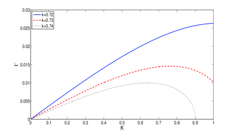
Figure 1: The instability growth rate given by Eq. (17) is shown at different wave numbers of the carrier drift mode. The parameter values are $\alpha=\gamma=0.05$.

Excat solutions of the NLSE (12) can be obtained by considering $\Phi=\sqrt{\Psi}\exp(i\theta)$, where $\Psi$ and $\theta$ are real functions to be determined (see for details, e.g., Refs. [21]). For $PQ>0$ the drift wave is modulationally unstable leading to the formation of bright envelope modulated wave packets given by (Fig. 2)

$$\Psi=\Psi_{0}\hskip 1.0pt\text{sech}^{2}\left(\frac{\xi-U\tau}{W}\right),\hskip 2.0pt\theta=\frac{1}{2P}\left[U\xi+\left(\Omega_{0}-\frac{U^{2}}{2}\right)\tau\right],$$ (18)

which represents a localized pulse traveling at a speed $U$ and oscillating at a frequency $\Omega_{0}$ at rest. The pulse width $W$ is related to the constant amplitude $\Psi_{0}$ as $W=\sqrt{2P/Q\Psi_{0}}$.

Figure 2: The evolution of the bright envelope soliton as given by Eq. (18) at $\tau=0$ for $k=0.71$, $\alpha=\gamma=0.05$, $\Psi_{0}=0.04$ and $U=0.5$.

On the other hand, for $PQ<0$, the modulationally stable drift wave packet will propagate in the form of a dark envelope soliton characterized by a depression of the drift wave potential around $\xi=0$. This is given by (Fig. 3)

$$\Psi=\Psi_{1}\hskip 1.0pt\text{tanh}^{2}\left(\frac{\xi-U\tau}{W_{1}}\right),$$

$$\theta=\frac{1}{2P}\left[U\xi-\left(\frac{U^{2}}{2}-2PQ\Psi_{1}\right)\tau\right],$$ (19)

representing a localized region of hole (void) traveling at a speed $U$. The pulse width $W_{2}$ depends on the constant amplitude $\Psi_{1}$ as $W_{2}=\sqrt{2|P/Q|/\Psi_{1}}$.

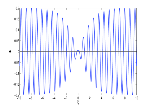
Figure 3: The evolution of the dark envelope soliton as given by Eq. (19) at $\tau=0$ for $k=0.5$, $\alpha=\gamma=0.05$, $\Psi_{0}=0.04$ and $U=0.5$.

Furthermore, the NLSE (12) has a rational solution that is located on a non-zero background and localized both in the $\tau$ and $\xi$ directions. For $PQ>0$ we have the drift rogue waves/rogons [22, 23]

$$\Phi=\Phi_{0}\left[\frac{4\left(1+2iQ\tau\right)}{1+4Q^{2}\tau^{2}+2Q\xi^{2}/P}-1\right]\exp\left(iQ\tau\right),$$ (20)

which reveals that a significant amount of energy is concentrated in a relatively small area in space. The typical form of the rogue wave is shown in Fig. 4. Hence, a random perturbation of the drift wave amplitude will grow on account of the modulational instability.

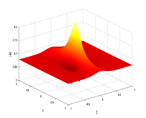
Figure 4: The evolution of the rogon as given by Eq. (20) at $k=0.72$ with parameters $\alpha=\gamma=0.05$.

To summarize, we have considered the amplitude modulation of a finite amplitude one-dimensonal electrostatic drift wave packet in a nonunform magnetoplasma in presence of equilibrium density, electron temperature and magnetic field gradients. It is shown that the dynamics of the modulated drift wave packet is governed by a nonlinear Schrödinger equation. Since the group dispersion of the drift waves is always negative for $k<1$, the formation of the bright envelope drift wave soliton or drift rogons is possible only when $Q<0$, which happens for $0.71\lesssim k\lesssim 1$. In the opposite case, viz. $0<k<0.71$ when $Q>0$, an amplitude modulated drift wave packet is stable and it propagates in the form of a dark envelope soliton [24]. In conclusion, the present results should be helpful in identifying modulated drift wave packets that may spontaneously emerge in magnetized space and laboratory plasmas that contain equilibrium density, electron temperature and magnetic field inhomogeneities.

References

- [1] B.B. Kadomtsev, Plasma Turbulence (Academic, New York, 1965).
- [2] J. Weiland, Collective Modes in Inhomogeneous Plasma: Kinetic and Advanced Fluid Theory (Institute of Physics, Bristol, 2000).
- [3] W. Horton, Rev. Mod. Phys. 71 (1999) 735; W. Horton and A. Hasegawa, Chaos 4 (1994) 227.
- [4] V.I. Petviashvili and O.A. Pokhotelov, Sov. J. Plasma Phys. 12 (1986) 657; Solitary Waves in Plasmas and in the Atmosphere (Gordon and Breach, Langhorne, 1992).
- [5] D. Sundqvist, V. Krasnoselskikh, P.K. Shukla et al., Nature (London) 436 (2005) 825; D. Sundkvist and S.D. Bale, Phys. Rev. Lett. 101 (2008) 065001.
- [6] N. Vianello, M. Spolaore, E. Martines et al., Nucl. Fusion 50 (2010) 042002.
- [7] C. Theiler, L. Furno, J. Loizu and A. Fasoli, Phys. Rev. Lett. 108 (2012) 065005.
- [8] H. Tasso, Phys. Lett. A 24 (1967) 618.
- [9] V.N. Orevskii, H. Tasso, and H. Wobig, in Proc. 3rd International Conference on Plasma Physics and Controlled Nuclear Fusion Research, Novosibirsk, USSR, 1968, International Atomic Energy, Vienna, Vol. 1, p. 671 (1969).
- [10] V.I. Petviashvili, Sov. J. Plasma Phys. 3 (1977) 150.
- [11] K. Mima and A. Hasegawa, Phys. Rev. Lett. 39 (1977) 205; A. Hasegawa and K. Mima, Phys. Fluids 21 (1978) 87.
- [12] J. G. Charney, J. Meteor. 4 (1947) 135; J. Atmos. Sci. 28 (1971) 1087.
- [13] V.D. Larichev and Rezhnik, Dyn. Atmos. Ocean 5 (1981) 219.
- [14] P.K. Shukla, Phys. Scr. 36 (1987) 644.
- [15] D. Jovanovic and W. Horton, Phys. Fluids B 5 (1993) 9.
- [16] P.K. Shukla, H.U. Rahman, M.Y. Yu, and K.H. Spatschek, Phys. Rev. A 23 (1981) 321; Phys. Rep. 105 (1984) 227.
- [17] G.R. Tynan, A. Fujisawa, and G. McKee, Plasma Phys. Control. Fusion 51 (2009) 113001.
- [18] T. Taniuti and N. Yajima, J. Math. Phys. 10 (1969) 1369; N. Asano, T. taniuiti, and N. Yajima, ibid. 10 (1969) 2020.
- [19] Y. Ichikawa and T. Taniuti, J. Phys. Soc. Jpn. 34 (1973) 513.
- [20] M. Kao, Prog. Theor. Phys. 55 (Suppl.) (1974) 120; T. Taniuti, ibid. 55 (Suppl.) (1974) 1; T. Kakutani and N. Sugimoto, Phys. Fluids 17 (1974) 1617.
- [21] I. Kourakis and P.K. Shukla, Nonlinear Processes in Geophysics, 12 (2005) 1; R. Fedele et al, Phys. Scr. T98 (2002) 18; idem, Eur. Phys. J. B 27 (2002) 313.
- [22] A. Ankiewicz, N. Devine, and N. Akhmediev, Phys. Lett. A 373 (2009) 3997; N. Akhemediev, J.M. Soto-Crespo, and A. Ankiewicz, Phys. Rev. A 80 (2009) 043818.
- [23] L. Stenflo and M. Marklund, J. Plasma Phys. 76 (2010) 293.
- [24] R. Fedele, Phys. Scr. 65 (2002) 502.