Fully massive Scheme for Jet Production in DIS

Abstract

We present a consistent treatment of heavy quarks for jet production in DIS at NLO accuracy. The method is based on the ACOT massive factorization scheme and dipole subtraction method for jets. The last had to be however extended in order to take into account initial state splittings with heavy quarks. We constructed relevant kinematics and dipole splitting functions together with their integrals. We partially implemented the method in a MC program and checked against the known inclusive result for charm structure function.

1 Introduction

There are two basic approaches to heavy quarks production in DIS. First is so called zero-mass variable flavor number scheme (ZM-VFNS), which treats heavy quarks as massless partons with corresponding parton distribution functions (PDF). This scheme is applicable when the hard scale (taken here as the virtuality of the exchanged boson $Q^{2}$) is much larger then the mass $m_{\mathbf{Q}}$ of a given heavy quark $\mathbf{Q}$. On the other hand, when $Q^{2}$ is of the order of $m_{\mathbf{Q}}$, so called fixed flavor number scheme (FFNS) is applicable. It retains the full mass dependence in the coefficient function and there is no PDF for $\mathbf{Q}$ as to the leading power it cannot appear in the soft part.

Increasing precision of the data forces us to control also the intermediate region of $Q^{2}$. The methods that address this problem are called general mass schemes (GM) [1, 2, 3, 4]. They are however formulated for inclusive processes only and similar method relevant for jets is highly desirable.

In the following we briefly describe our solution to this problem [5, 6]. It is based on the ACOT massive factorization theorem [1, 7] and massive dipole subtraction method (DSM) [8, 9, 10], which however had to be reformulated in order to match with the former.

2 Dipole subtraction method with massive partons

Consider NLO calculation of a cross section for producing $n$ jets in lepton-hadron reaction. The LO cross section is schematically written as

$$\sigma_{n}^{\left(\mathrm{LO}\right)}=\mathcal{N}\,\sum_{a}f_{a}\otimes\,\int d\Phi_{n,a}\,\left|\mathcal{M}_{n,a}\right|^{2}F_{n,a},$$ (1)

where $\mathcal{N}$ is a normalization factor, $f_{a}$ are PDFs, $d\Phi_{n,a}$ is $n$-parton phase space (PS) and $\mathcal{M}_{n,a}$ is a tree-level matrix element (ME) with $n$ final state partons and one QCD initial state parton $a$. The jet function $F_{n,a}$ determines the actual observable and is realized by a suitable jet algorithm. It satisfies $F_{n+1,a}=F_{n,a}$ in the singular regions of PS. At NLO the corrections involve loop diagrams living on $n$-particle PS and additional real emission belonging to $\left(n+1\right)$-particle PS. Both contain IR singularities which ultimately cancel, however the cancellation is non-trivial as the singularities have different origin. An elegant and exact solution is provided by DSM. One adds and subtracts an auxiliary contribution $\mathcal{D}_{n,a}$, such that it mimics all the singularities of $\mathcal{M}_{n+1,a}$ and at the same time can be analytically integrated over singular regions of PS. To be more specific we have

$$\sigma_{n}^{\left(\mathrm{NLO}\right)}=\mathcal{N}\,\sum_{a}f_{a}\otimes\Bigg{\{}\int d\Phi_{n+1,a}\,\left[\left|\mathcal{M}_{n+1,a}\right|^{2}F_{n+1,a}-\mathcal{D}_{n,a}F_{n,a}\right]\\ +\int d\Phi_{n,a}\,\left[\mathcal{M}_{n,a}^{\left(\mathrm{loop}\right)}+\int d\phi_{a}\,\mathcal{D}_{n,a}-\mathcal{C}_{n,a}\right]\,F_{n,a}\Bigg{\}},$$ (2)

where virtual corrections to $\left|\mathcal{M}_{n,a}\right|^{2}$ are symbolically denoted as $\mathcal{M}_{n,a}^{\left(\mathrm{loop}\right)}$. The subspace leading to singularities is $d\phi_{a}$ and fulfils PS factorization formula $d\Phi_{n+1,a}=d\Phi_{n,a}\otimes d\phi_{a}$. Thanks to the properties of $\mathcal{D}_{n,a}$ and $F_{n+1,a}$ the first square bracket is integrable in four dimensions, while in the second, the poles resulting from integral $\int d\phi_{a}\,\mathcal{D}_{n,a}$ are cancelled against the ones in $\mathcal{M}_{n,a}^{\left(\mathrm{loop}\right)}$. However, not all singularities cancel in this way – there are also collinear poles connected with initial state splittings of massless partons. They are removed by means of collinear subtraction term $\mathcal{C}_{n,a}$. It has the form

$$\mathcal{C}_{n,a}=\sum_{b}\mathcal{F}_{ab}\otimes\left|\mathcal{M}_{n,b}\right|^{2},$$ (3)

where $\mathcal{F}_{ab}$ are renormalized partonic PDFs, i.e. the densities of partons $b$ inside parton $a$. For instance in the $\overline{\mathrm{MS}}$ scheme $\mathcal{F}_{ab}\left(z\right)=-\frac{1}{\varepsilon}\,\frac{\alpha_{s}}{2\pi}\,P_{ab}\left(z\right)$, where $P_{ab}\left(z\right)$ are standard splitting functions.

Within DSM the dipole function is realized as a sum of contributions corresponding to single emissions with different combinations of “emitter” and “spectator”partons. Each such term $D$ has a general form

$$D=\hat{V}\,\hat{C}\left|\hat{\mathcal{M}}_{n,a}\right|^{2},$$ (4)

where $\hat{V}$ is so called dipole splitting matrix (in helicity space) and encodes the information about some of the singularities of $\mathcal{M}_{n+1,a}$. The matrix $\hat{C}$ corresponds to color operators for parton emissions, which act on the matrix element. The notation above is symbolic and means that both quantities are correlated in the color and spin space. For DIS, there are three different classes of dipoles $D$, depending on whether emitter or spectator are in the initial or final states. Here we are mainly interested in the case of initial state emitter and final state spectator as they contain factorization-related information.

When heavy quarks are present, the above general picture remains the same. If however a massive parton takes part in a splitting process there is no collinear singularity. Nevertheless there are IR sensitive logarithms which become harmful when the external scale becomes large. We shall refer to such terms as quasi-collinear singularities [12] and abbreviate as q-singularities.

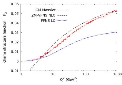
Figure 1: ACOT charm structure function calculated using MC implementation of our method ($\mathtt{MassJet}$). The calculations are done for $x_{B}=0.05$ and CTEQ5 PDFs.

The first step towards GM scheme for jets is to construct dipole functions controlling q-singularities for initial state emissions. Moreover we want to have possibly massive initial states as it is allowed by the ACOT scheme. It was partially done in [8] (for $\mathbf{Q}\rightarrow\mathbf{Q}g$ splitting), while in [10] the splitting processes with heavy quarks are considered in the final states only.

Let us look at the particular example. Consider the initial state $g\rightarrow\mathbf{Q}\overline{\mathbf{Q}}$ splitting. Let us assign the momentum $p_{a}$ to the gluon, $p_{i}$ to the emitted final state quark (or anti-quark), and $p_{j}$ to the spectator. Using these, we construct new momenta which enter $\mathcal{M}_{n,a}$ in (4): $\tilde{p}_{j}^{\mu}=\tilde{w}\left(p_{i}^{\mu}+p_{j}^{\mu}\right)-\tilde{u}p_{a}^{\mu}$ becomes a new final state and $\tilde{p}_{\underline{ai}}^{\mu}=\left(\tilde{w}-1\right)\left(p_{i}^{\mu}+p_{j}^{\mu}\right)-\left(\tilde{u}-1\right)p_{a}^{\mu}$ becomes a new initial state. The variables $\tilde{u}$, $\tilde{w}$ can be determined from on-shell conditions for $\tilde{p}_{j}$ and $\tilde{p}_{\underline{ai}}$. Our dipole splitting function reads

$$\hat{V}_{g\rightarrow\mathbf{Q}\overline{\mathbf{Q}},\,j}=8\pi\mu_{\mathrm{r}}^{2\varepsilon}\alpha_{s}T_{R}\left[1-\frac{1}{1-\varepsilon}\,\left(2\tilde{u}\left(1-\tilde{u}\right)-\frac{\left(1-\tilde{u}\right)m_{\mathbf{Q}}^{2}}{p_{i}\cdot p_{a}}\right)\right],$$ (5)

where $\mu_{r}$ is a mass scale needed in $D=4-2\varepsilon$ dimensions. In this case $\hat{V}$ is just diagonal in helicity space.

Consider next the integral of (5) over one-particle subspace. It can be convenietly expressed in terms of rescaled masses $\eta_{l}^{2}=m_{l}^{2}/2\tilde{p}_{j}\cdot p_{a}$ for some parton $l$. In the limit of small $\eta_{\mathbf{Q}}$ we get

$$\int d\phi\,\hat{V}_{g\rightarrow\mathbf{Q}\overline{\mathbf{Q}},\,j}\left(u\right)=\frac{\alpha_{s}}{2\pi}\Bigg{[}P_{gq}\left(u\right)\Bigg{(}\log\frac{u^{2}}{u+\eta_{j}^{2}}-\log\eta_{\mathbf{Q}}^{2}\Bigg{)}+2T_{R}\,u\left(1-u\right)\Bigg{]}+\mathcal{O}\left(\eta_{\mathbf{Q}}^{2}\right).$$ (6)

We see that there is a term of the form $P_{gq}\left(u\right)\log\eta_{\mathbf{Q}}^{2}$ which becomes harmful when the scale becomes large (in massless case there would be a pole $1/\varepsilon$). Similar terms appear also in other dipoles for the initial state emissions.

3 General mass scheme for jets

In the spirit of the ACOT scheme, the initial state q-singularities have to be factorized out. It is accomplished by $\mathcal{C}_{n,a}$ term with partonic PDFs $\mathcal{F}_{ab}$ calculated in a special way. Let us recall at this point, that the latter are defined as certain ME of light-cone operators and can be calculated order by order using special Feynman rules (see e.g. [13]). The results contain UV singularities which have to be renormalized, leading to evolution equations. For the present application we calculate $\mathcal{F}_{ab}$ to one loop with full mass dependence and renormalize them using the $\overline{\mathrm{MS}}$ scheme. Since counterterms are mass independent in this scheme, we assure that hadronic PDFs evolve according to standard massless DGLAP equations. For instance we get

$$\mathcal{F}_{g\mathbf{Q}}\left(z\right)=\frac{\alpha_{s}}{2\pi}\,T_{R}\,\left(1-2z\left(1-z\right)\right)\,\log\frac{\mu_{r}^{2}}{m_{\mathbf{Q}}^{2}},$$ (7)

$$\mathcal{\mathcal{F}}_{\mathbf{Q}g}\left(z\right)=\frac{\alpha_{s}}{2\pi}\,C_{F}\,\frac{1+\left(1-z\right)^{2}}{z}\left[\log\frac{\mu_{r}^{2}}{m_{\mathbf{Q}}^{2}}-2\log z-1\right],$$ (8)

$$\mathcal{\mathcal{F}}_{\mathbf{Q}\mathbf{Q}}\left(z\right)=\frac{\alpha_{s}}{2\pi}\,C_{F}\left\{\frac{1+z^{2}}{1-z}\left[\log\frac{\mu_{r}^{2}}{m_{\mathbf{Q}}^{2}}-2\log\left(1-z\right)-1\right]\right\}_{+}.$$ (9)

We have checked that the above procedure leads to IR safe dipoles in the limit of vanishing $\eta_{\mathbf{Q}}$. Moreover, the results coincide with those Ref. [10] in the $\overline{\mathrm{MS}}$ scheme.

In order to perform numerical tests we have partially implemented our method in a dedicated C++ program based on FOAM [14]. Using the program, we have calculated the charm structure function $F_{2}$ and compared it with semi-analytical calculation in the ACOT scheme. This exercise uses three dipoles and two collinear subtraction terms. The virtual corrections are taken from [15]. We find that the soft poles are indeed cancelled by the corresponding poles coming from the integrated dipoles. Moreover, we find agreement with the semi-analytical calculation and observe that our result properly interpolates between the two limiting solutions of the ZM-VFNS and FFNS schemes, as depicted in Fig. 1.

Let us stress that the result is obtained by a numerical integration of a fully differential cross section, which provides a severe test on the implementation of our massive dipole formalism.

References

- [1] M. A. G. Aivazis, J. C. Collins, F. I. Olness, and W.-K. Tung. Phys. Rev. D50 (1994) 3102–3118, arXiv:hep-ph/9312319.
- [2] M. Buza, Y. Matiounine, J. Smith, and W. L. van Neerven. Eur. Phys. J. C1 (1998) 301–320, arXiv:hep-ph/9612398.
- [3] R. S. Thorne and R. G. Roberts. Phys. Rev. D57 (1998) 6871–6898, arXiv:hep-ph/9709442.
- [4] S. Forte, E. Laenen, P. Nason, and J. Rojo. Nucl.Phys. B834 (2010) 116–162, arXiv:1001.2312 [hep-ph].
- [5] P. Kotko, General Mass Scheme for Jet production in QCD. PhD thesis, Jagiellonian Univ., 2012.
- [6] P. Kotko and W. Slominski. In preparation.
- [7] J. C. Collins. Phys. Rev. D58 (1998) 094002, arXiv:hep-ph/9806259.
- [8] S. Dittmaier. Nucl. Phys. B565 (2000) 69–122, arXiv:hep-ph/9904440.
- [9] L. Phaf and S. Weinzierl. JHEP 0104 (2001) 006, arXiv:hep-ph/0102207 [hep-ph].
- [10] S. Catani, S. Dittmaier, M. H. Seymour, and Z. Trocsanyi. Nucl. Phys. B627 (2002) 189–265, arXiv:hep-ph/0201036.
- [11] S. Catani and M. H. Seymour. Nucl. Phys. B485 (1997) 291–419, arXiv:hep-ph/9605323. Erratum: ibid. B510:503-504,1998; [arXiv:hep-ph/9605323v3] includes changes from the Erratum.
- [12] S. Catani, S. Dittmaier, and Z. Trocsanyi. Phys. Lett. B500 (2001) 149–160, arXiv:hep-ph/0011222.
- [13] J. Collins, Foundations of perturbative QCD, vol. 32. Cambridge Univ. Press, 2011.
- [14] S. Jadach. Comput. Phys. Commun. 152 (2003) 55–100, arXiv:physics/0203033.
- [15] S. Kretzer and I. Schienbein. Phys. Rev. D58 (1998) 094035, arXiv:hep-ph/9805233.