Optical properties of bulk semiconductors and graphene/boron-nitride: The Bethe-Salpeter equation with derivative discontinuity-corrected DFT energies

Abstract

We present an efficient implementation of the Bethe-Salpeter equation (BSE) for optical properties of materials in the projector augmented wave method GPAW. Single-particle energies and wave functions are obtained from the GLLBSC functional which explicitly includes the derivative discontinuity, is computationally inexpensive, and yields excellent fundamental gaps. Electron-hole interactions are included through the BSE using the statically screened interaction evaluated in the random phase approximation. For a representative set of semiconductors and insulators we find excellent agreement with experiments for the dielectric functions, onset of absorption, and lowest excitonic features. For the two-dimensional systems of graphene and hexagonal boron-nitride (h-BN) we find good agreement with previous many-body calculations. For the graphene/h-BN interface, we find that the fundamental and optical gaps of the h-BN layer are reduced by 2.0 eV and 0.7 eV, respectively, compared to freestanding h-BN. This reduction is due to image charge screening which shows up in the GLLBSC calculation as a reduction (vanishing) of the derivative discontinuity.

I Introduction

Optical spectroscopies such as photo absorption, luminescence, and reflectance measurements are widely used for materials characterization. In this context, first-principles calculations play an increasingly important role for the interpretation and guidance of experimental investigations. However, theoretical spectroscopic methods are not only useful for characterization purposes. Indeed, with the recent focus on solar energy conversion, plasmonics, and optoelectronics – all applications which involve the interaction of light with matter – first-principles methods for calculating the optical properties of complex materials are becoming the essential tool allowing for reliable computational design of new materials within these areas.

The two most commonly used ab-initio methods for optical properties are time-dependent density functional theory (TDDFT)Runge and Gross (1984) and many-body perturbation theory (MBPT)Onida et al. (2002). For smaller molecules and clustersCasida et al. (1998), TDDFT with the adiabatic local density approximation (ALDA) provides a reasonably good compromise between accuracy and computational cost. However, the ALDA fails to describe several important effects including the formation of excitons in extended systemsBotti et al. (2007), charge-transfer excitations in donor-acceptor molecular complexesDreuw et al. (2003); Garcia-Lastra and Thygesen (2011), as well as the screening of optical transitions by nearby metal surfacesGarcia-Lastra and Thygesen (2011). Apart from these qualitative failures, the ALDA is also found to underestimate the optical transition energies and overestimate static dielectric constants of bulk insulators and semiconductors. This problem is, at least to some extent, related to the well known tendency of the LDA and related semi local exchange-correlation (xc) functionals, to underestimate the fundamental energy gaps in such systems.

All of the above mentioned problems of the TDDFT-ALDA approach are overcomed by the MBPT. In the standard scheme, the quasiparticle band structures are obtained using the GW approximationAryasetiawan and Gunnarsson (1998) while optical excitation energies are obtained by solving a Bethe-Salpeter equation (BSE)Salpeter and Bethe (1951) with a statically screened electron-hole interaction. The GW-BSE approachAlbrecht et al. (1998); Rohlfing and Louie (2000) has been succesfully applied to a number of different systems ranging from bulk semiconductorsAlbrecht et al. (1998), insulators and their surfacesRohlfing and Louie (1999), two-dimensional systems such as grapheneYang et al. (2009) and boron nitride layersArnaud et al. (2006), metal-molecule interfacesGarcia-Lastra and Thygesen (2011), isolated moleculesOnida et al. (1995); Rohlfing and Louie (1998); del Puerto et al. (2006) and liquid waterGarbuio et al. (2006). Nevertheless, applications of the approach to larger systems are limited by the extremely demanding computational requirements of both the GW and BSE calculations.

Several schemes have been proposed to reduce the computational cost of GW-BSE calculations. These include circumventing the GW step by applying simpler band structures e.g. derived from the COHSEX approximationHedin (1965) or simply scissors operator-corrected LDA band structuresLevine and Allan (1989), or the use of model dielectric functions to describe the screeningHybertsen and Louie (1986). Another route of research is directed towards the development of more accurate TDDFT xc-kernels without sacrificing the computational simplicity associated with this approachMarini et al. (2003); Turkowski et al. (2009); Sharma et al. (2011).

Recently, Kuisma et al. have introduced the GLLBSC xc-potentialKuisma et al. (2010) which is based on an earlier functional developed by Gritsenko et al.Gritsenko et al. (1995). This potential explicitly includes the derivative discontinuity of the xc-potential at integer particle numbers which is important to obtain physically meaningful band gaps from DFT. The derivative discontinuity, $\Delta_{\mathrm{xc}}$, is calculated directly from the Kohn-Sham eigenvalues and eigenstates. The fundamental band gap is then obtained as the sum of the Kohn-Sham single-particle gap and the derivative discontinuity. The GLLBSC method has been shown to produce fundamental band gaps as well as band dispersions for a range of semiconductors in very good agreement with experiments and more sophisticated theoretical approaches while the computational cost is comparable to that of LDAKuisma et al. (2010); Castelli et al. (2012); Yan et al. (2011a).

In this paper we combine the TDDFT and BSE methods for treating the electron-hole interaction with the GLLBSC method for the wave function and band structures. Considering both bulk and low dimensional systems we find that the accuracy of the GLLBSC-BSE approach is comparable to the GW-BSE approach. All the methods are implemented in the gpaw codeMortensen et al. (2005); Enkovaara et al. (2010); Yan et al. (2011b), an electronic structure package based on the projector augmented wave methodologyBlöchl (1994); Blöchl et al. (2003). For the bulk systems Si, C, InP, MgO, GaAs and LiF, we find that the fundamental gaps and static dielectric constants calculated with GLLBSC compare well with experimental data. Importantly, the static dielectric constant should be evaluated without the derivative discontinuity when using an xc-kernel that does not account for e-h interaction such as the ALDA or the random phase approximation (RPA). The experimental optical absorption spectra of all compounds are also very well reproduced by the GLLBSC-BSE approach including the absorption onset and excitonic peaks. Finally, the method is used to compute the band structure and optical absorption spectra of graphene, hexagonal boron-nitride (h-BN), and a graphene/h-BN interface. For the isolated sheets we find good agreement with previous GW-BSE calculations. For the interface we find that both the quasiparticle- and optical gap of the h-BN sheet are reduced by 2.0 and 0.7 eV, respectively. The physical origin of this effect is due to image charge screening by the graphene layer. In the GLLBSC, the reduction shows up as a vanishing of the derivative discontinuity.

The rest of the paper is organized as follows. Section II introduces the theoretical framework for calculating optical properties of solids with gpaw using the TDDFT and BSE approaches, followed by a brief review of the GLLBSC method. Details of the implementation are presented in Sec. III. Section IV presents benchmark results for the band gaps, dielectric constants and optical absorption spectra of a number of bulk semiconductors and insulators. In Sec. V we present the band structures and optical spectra of graphene, h-BN, and graphene/h-BN interface. Finally, a summary is given in Sec. V.

II Method

II.1 Macroscopic dielectric function

Most of the optical properties of a solid can be obtained from the macroscopic dielectric function,

$$\epsilon(\omega)\equiv\left.\frac{1}{\epsilon^{-1}_{\bm{\mathrm{G}}\bm{\mathrm{G}}^{\prime}}(\bm{\mathrm{q}}\rightarrow 0,\omega)}\right|_{\bm{\mathrm{G}}=0,\bm{\mathrm{G}}^{\prime}=0}.$$ (1)

Here, $\epsilon_{\bm{\mathrm{G}}\bm{\mathrm{G}}^{\prime}}(\bm{\mathrm{q}},\omega)$ is the (microscopic) dielectric matrix in reciprocal $\bm{\mathrm{G}}$ space. The off-diagonal elements of the $\epsilon$ matrix account for local field effects arising due to the periodic crystal potential. The macroscopic average is achieved through the inversion of the $\epsilon$ matrix.

In this work we consider only the longitudinal component of the dielectric function. For applications to optical properties this is in fact not a restriction because in the relevant long wave length limit the electrons do not feel the difference between longitudinal and transversely polarized fields, and consequently the two types of response functions coincide. Still, for anisotropic systems $\epsilon(\omega)$ depends on the direction in which the limit $\bm{\mathrm{q}}\to 0$ is taken. However, to keep the notation simple we shall omit reference to this direction in what follows.

II.2 Linear response function from TDDFT

The microscopic dielectric matrix is related to the linear density response function, $\chi$, via

$$\epsilon^{-1}_{\mathbf{G}\mathbf{G}^{\prime}}(\mathbf{q},\omega)=\delta_{\mathbf{G}\mathbf{G}^{\prime}}+\frac{4\pi}{|\mathbf{q}+\mathbf{G}||\mathbf{q}+\mathbf{G}^{\prime}|}\chi_{\mathbf{G}\mathbf{G}^{\prime}}(\mathbf{q},\omega).$$ (2)

Within TDDFT the response function is related to the response function of the non-interacting Kohn-Sham electrons, $\chi^{0}$ and the exchange-correlation interaction kernel $K_{xc}$ via a Dyson-like equation,

$$\chi_{\mathbf{G}\mathbf{G}^{\prime}}(\mathbf{q},\omega)=\chi^{0}_{\mathbf{G}\mathbf{G}^{\prime}}(\mathbf{q},\omega)$$

$$+\sum_{\mathbf{G}_{1}\mathbf{G}_{2}}\chi^{0}_{\mathbf{G}\mathbf{G}_{1}}(\mathbf{q},\omega)K_{\mathbf{G}_{1}\mathbf{G}_{2}}(\mathbf{q},\omega)\chi_{\mathbf{G}_{2}\mathbf{G}^{\prime}}(\mathbf{q},\omega).$$ (3)

The KS response function is given byAdler (1962); Wiser (1963),

$$\chi^{0}_{\mathbf{G}\mathbf{G}^{\prime}}(\mathbf{q},\omega)=\frac{2}{\Omega}\sum_{\bm{\mathrm{k}},nn^{\prime}}(f_{n\mathbf{k}}-f_{n^{\prime}\mathbf{k}+\bm{\mathrm{q}}})$$

$$\times\frac{n_{n\bm{\mathrm{k}},n^{\prime}\mathbf{k}+\mathbf{q}}(\bm{\mathrm{G}})n^{\ast}_{n\bm{\mathrm{k}},n^{\prime}\mathbf{k}+\mathbf{q}}(\bm{\mathrm{G}}^{\prime})}{\omega+\epsilon_{n\mathbf{k}}-\epsilon_{n^{\prime}\mathbf{k}+\bm{\mathrm{q}}}+i\eta}$$ (4)

where $\varepsilon_{n\mathbf{k}}$ is a KS eigenvalue, and $f_{n\mathbf{k}}$ is the occupation factor. The quantity

$$n_{n\bm{\mathrm{k}},n^{\prime}\mathbf{k}+\mathbf{q}}(\bm{\mathrm{G}})\equiv\langle\psi_{n\mathbf{k}}|e^{-i(\bm{\mathrm{q}}+\bm{\mathrm{G}})\cdot\mathbf{r}}|\psi_{n^{\prime}\bm{\mathrm{k}}+\bm{\mathrm{q}}}\rangle$$ (5)

is referred to as the charge density matrixYan et al. (2011b). In the long wavelength limit, i.e. for $\bm{\mathrm{q}}\rightarrow 0$, and for $n\neq n^{\prime}$, application of the $k\cdot p$ perturbation theoryGrosso and Parravicini (2000) yields the important identity

$$\mathrm{lim}_{\bm{\mathrm{q}}\rightarrow 0}n_{n\bm{\mathrm{k}},n^{\prime}\bm{\mathrm{k}}+\bm{\mathrm{q}}}(0)=\frac{-i\bm{\mathrm{q}}\cdot\langle\psi_{n\mathbf{k}}|\nabla|\psi_{n^{\prime}\bm{\mathrm{k}}}\rangle}{\epsilon_{n^{\prime}\bm{\mathrm{k}}}-\epsilon_{n\bm{\mathrm{k}}}}.$$ (6)

Alternatively, this form follows directly if we consider the density induced by a longitudinal vector potential rather than a scalar potential. A detailed description of the evaluation of the charge density matrix and the ALDA xc-kernel within the PAW formalism can be found in Ref. Yan et al., 2011b.

II.3 The Bethe-Salpeter Equation

Several of the shortcomings of the ALDA in describing optical spectra are overcomed by explicitly accounting for electron self-energy effects and electron-hole interactions using many-body perturbation theory. In the standard GW-BSE approach, the single-particle energies are evaluated using a self-energy in the GW approximation while the optical excitation energies are obtained by diagonalizing an effective two-particle Hamiltonian. In the present work we avoid calculating the GW self-energy by using single-particle energies obtained from the efficient GLLBSC functional.

Following the standard approach, the excitation energies corresponding to an external potential with momentum $\bm{\mathrm{q}}$ can be found by solving an eigenvalue problem of the form

$$\sum_{S^{\prime}}\mathcal{H}(\bm{\mathrm{q}})_{SS^{\prime}}A_{S^{\prime}}^{\lambda}(\bm{\mathrm{q}})=E^{\lambda}(\bm{\mathrm{q}})A^{\lambda}_{S}(\bm{\mathrm{q}})$$ (7)

where $\mathcal{H}_{SS^{\prime}}(\bm{\mathrm{q}})$ is the Bethe-Salpeter effective two-particle Hamiltonian evaluated in a basis of electron-hole states, $\psi_{S}(\bm{\mathrm{r}}_{h},\bm{\mathrm{r}}_{e})=\psi_{n\bm{\mathrm{k}}}(\bm{\mathrm{r}}_{h})^{*}\psi_{m\bm{\mathrm{k}}+\bm{\mathrm{q}}}(\bm{\mathrm{r}}_{e})$. The BSE Hamiltonian reads

$$\mathcal{H}_{SS^{\prime}}(\bm{\mathrm{q}})=(\varepsilon_{m\bm{\mathrm{k}}+\bm{\mathrm{q}}}^{QP}-\varepsilon_{n\bm{\mathrm{k}}}^{QP})\delta_{SS^{\prime}}-(f_{m\bm{\mathrm{k}}+\bm{\mathrm{q}}}-f_{n\bm{\mathrm{k}}})K_{SS^{\prime}}(\bm{\mathrm{q}})$$ (8)

The kernel consists of an e-h exchange interaction ($V$) and a direct screened e-h attraction ($W$),

$$K_{SS^{\prime}}(\bm{\mathrm{q}})= V_{SS^{\prime}}(\bm{\mathrm{q}})-\frac{1}{2}W_{SS^{\prime}}(\bm{\mathrm{q}}).$$ (9)

The factor 2 accounts for spin. In appendix A we give a derivation of the BSE eigenvalue equation and its relation to the dielectric function.

The effective two particle Hamiltonian is most conveniently evaluated in a plane wave basis. In this representation the e-h exchange term reads

$$V_{SS^{\prime}}(\bm{\mathrm{q}})=\frac{4\pi}{\Omega}\sum_{\bm{\mathrm{G}}}\frac{n^{\ast}_{n\bm{\mathrm{k}},m\bm{\mathrm{k}}+\bm{\mathrm{q}}}(\bm{\mathrm{G}})n_{n^{\prime}\bm{\mathrm{k}}^{\prime},m^{\prime}\bm{\mathrm{k}}^{\prime}+\bm{\mathrm{q}}}(\bm{\mathrm{G}})}{|\bm{\mathrm{q}}+\bm{\mathrm{G}}|^{2}},$$ (10)

If we exclude the $\bm{\mathrm{G}}=0$ component in the sum we obtain the short range exchange kernel $\bar{V}$. The difference between $V$ and $\bar{V}$ becomes important when the response function is written in terms of the eigenstates and energies of the BSE Hamiltionian, see below. To obtain the optical limit $V_{SS^{\prime}}(\bm{\mathrm{q}}\to 0)$ we use the expression Eq. (6) to cancel the $1/q^{2}$ Coulomb divergence appearing in the $\bm{\mathrm{G}}=0$ term. In the evaluation of the remaining terms we use a small finite value for $\mathbf{q}$ (a value of 0.0001 Å^-1 has been used in this work).

The plane wave expression for the e-h direct Coulomb term reads

$$W_{SS^{\prime}}(\bm{\mathrm{q}}) =\frac{4\pi}{\Omega}\sum_{\bm{\mathrm{G}}\bm{\mathrm{G}}^{\prime}}n^{\ast}_{n\bm{\mathrm{k}},n^{\prime}\bm{\mathrm{k}}^{\prime}}(\bm{\mathrm{G}})W_{\bm{\mathrm{G}}\bm{\mathrm{G}}^{\prime}}(\bm{\mathrm{k}}^{\prime}-\bm{\mathrm{k}})$$

$$\times n_{m\bm{\mathrm{k}}+\bm{\mathrm{q}},m^{\prime}\bm{\mathrm{k}}^{\prime}+\bm{\mathrm{q}}}(\bm{\mathrm{G}}^{\prime}),$$ (11)

where

$$W_{\bm{\mathrm{G}}\bm{\mathrm{G}}^{\prime}}(\bm{\mathrm{k}}^{\prime}-\bm{\mathrm{k}})=\frac{\epsilon^{-1}_{\bm{\mathrm{G}}\bm{\mathrm{G}}^{\prime}}(\bm{\mathrm{k}}^{\prime}-\bm{\mathrm{k}},\omega=0)}{|\bm{\mathrm{k}}^{\prime}-\bm{\mathrm{k}}+\bm{\mathrm{G}}||\bm{\mathrm{k}}^{\prime}-\bm{\mathrm{k}}+\bm{\mathrm{G}}^{\prime}|}$$ (12)

Here we encounter a divergence of $W_{\bm{\mathrm{G}}\bm{\mathrm{G}}^{\prime}}$ when either $\bm{\mathrm{G}}$ or $\bm{\mathrm{G}}^{\prime}$ is zero and $\bm{\mathrm{k}}=\bm{\mathrm{k}}^{\prime}$. Such a divergence due to the singularity of the Coulomb kernel at $q=0$ is also present in calculating exact exchangeSpencer and Alavi (2008) and GW self energiesFreysoldt et al. (2007). When $n\neq n^{\prime}$ and $m\neq m^{\prime}$ we can use the expression Eq. (6) to cancel the divergence; while for $n=n^{\prime}$ or $m=m^{\prime}$, the singularity in the Coulomb kernel is integrated out analytically, following Ref. Hybertsen and Louie, 1986, around a sphere centered at $q=0$. We have also adopted another scheme using an auxiliary periodic function with the same singularity as the exact function but which can be evaluated analyticallyGygi and Baldereschi (1986). These two schemes give essentially the same results.

The eigenstates and eigenvalues of the BSE Hamiltonian provide a spectral representation of the four-point density response function (see Appendix A),

$$\chi_{SS^{\prime}}^{\text{4P}}(\bm{\mathrm{q}},\omega)=\sum_{\lambda\lambda^{\prime}}\frac{A_{S}^{\lambda}(\bm{\mathrm{q}})[A_{S^{\prime}}^{\lambda^{\prime}}(\bm{\mathrm{q}})]^{\ast}N^{-1}_{\lambda\lambda^{\prime}}}{\omega-E^{\lambda}(\bm{\mathrm{q}})+i\eta}$$ (13)

where $N_{\lambda\lambda^{\prime}}$ is the overlap matrix defined as

$$N_{\lambda\lambda^{\prime}}\equiv\sum_{S}[A_{S}^{\lambda}(\bm{\mathrm{q}})]^{\ast}A_{S}^{\lambda^{\prime}}(\bm{\mathrm{q}}).$$ (14)

Using the plane wave representation (5) of the electron-hole basis states we obtain the following expression for the response function in reciprocal space

$$\chi_{\bm{\mathrm{G}}\bm{\mathrm{G}}^{\prime}}(\bm{\mathrm{q}},\omega)=\frac{1}{\Omega}\sum_{SS^{\prime}}\chi^{\text{4P}}_{SS^{\prime}}(\bm{\mathrm{q}},\omega)n_{S}(\bm{\mathrm{G}})n^{\ast}_{S^{\prime}}(\bm{\mathrm{G}}^{\prime})$$ (15)

From this expression the inverse dielectric constant and macroscopic dielectric constant follows from Eq. (2) and (1), respectively.

We note that upon excluding the $1/q^{2}$ term in the e-h exchange term, i.e. replacing $V$ by $\bar{V}$ in the kernel (9), the eigenstates and eigenvalues of the BSE Hamiltonian provides a spectral representation of the irreducible response function rather than the full response function. In this case the effect of $\bar{V}$ is to account for local field effects. Consequently the macroscopic dielectric function can be written

$$\epsilon(\omega)=1-\frac{4\pi}{|\bm{\mathrm{q}}|^{2}}\bar{\chi}_{00}(\bm{\mathrm{q}}\rightarrow 0,\omega)$$ (16)

$$=1-\frac{4\pi}{\Omega|\bm{\mathrm{q}}|^{2}}\sum_{SS^{\prime}}n_{S}(0)n^{\ast}_{S^{\prime}}(0)f_{S^{\prime}}\sum_{\lambda\lambda^{\prime}}\frac{\bar{A}_{\lambda}^{S}(\bm{\mathrm{q}})[\bar{A}_{\lambda^{\prime}}^{S^{\prime}}(\bm{\mathrm{q}})]^{\ast}\bar{N}^{-1}_{\lambda\lambda^{\prime}}(\bm{\mathrm{q}})}{\omega-E_{\lambda}(\bm{\mathrm{q}})+i\eta}$$

In the above expression the optical limit $\bm{\mathrm{q}}\to 0$ is taken in the following way. First, the BSE Hamiltonian is constructed using an e-h basis of vertical excitations ($\bm{\mathrm{q}}=0$) but using a finite small $\bm{\mathrm{q}}$ for the Coulomb interaction $1/|\bm{\mathrm{q}}+\bm{\mathrm{G}}|$ in $V$ (or $\bar{V}$). The same finite $\bm{\mathrm{q}}$ is then used when evaluating the dielectric function from the spectral representation of the (irreducible) response function.

II.4 Quasiparticle energies from GLLBSC

The derivative discontinuity $\Delta_{\mathrm{xc}}$ is defined as the difference between the fundamental gap $E_{\mathrm{g}}$ and the Kohn-Sham (KS) single-particle gap $E_{\mathrm{g}}^{\mathrm{KS}}$ as follows

$$E_{\mathrm{g}}=I-A=E[n_{N-1}]-2E[n_{N}]+E[n_{N+1}]=E_{\mathrm{g}}^{\mathrm{KS}}+\Delta_{\mathrm{xc}},$$ (17)

where $E[n_{N}]$ is the total energy of the $N$-electron system and the fundamental band gap $E_{\mathrm{g}}$ is defined as the difference betweeen the ionization energy $I$ and the electron affinity $A$.

Within the GLLBSC method, the derivative discontinuity $\Delta_{\mathrm{xc}}$ is obtained through

$$\Delta_{\mathrm{xc}}=\langle\Psi_{N+1}|\Delta(\bm{\mathrm{r}})|\Psi_{N+1}\rangle$$ (18)

where

$$\Delta(\bm{\mathrm{r}})=\sum_{i}^{\mathrm{occ}}K_{x}\left[\sqrt{\epsilon_{\mathrm{LUMO}}-\epsilon_{i}}-\sqrt{\epsilon_{\mathrm{HOMO}}-\epsilon_{i}}\right]\frac{|\psi_{i}(\bm{\mathrm{r}})|^{2}}{n(\bm{\mathrm{r}})}.$$ (19)

$\epsilon_{i}$, $\psi_{i}(\bm{\mathrm{r}})$ and $n(\bm{\mathrm{r}})$ are eigenvalues, eigenstates and electron density, respectively, obtained from solving the KS equation with the following GLLBSC potential

$$v_{\mathrm{GLLBSC}}(\bm{\mathrm{r}}) =2\epsilon_{\mathrm{xc}}^{\mathrm{PBEsol}}(\bm{\mathrm{r}})$$ (20)

$$+\sum_{i}^{\mathrm{occ}}K_{x}\sqrt{\epsilon_{r}-\epsilon_{i}}\frac{|\psi_{i}(\bm{\mathrm{r}})|^{2}}{n(\bm{\mathrm{r}})}+v_{\mathrm{c,resp}}^{\mathrm{PBEsol}}(\bm{\mathrm{r}})$$

Here, $K_{x}\approx 0.382$ is a coefficient fitted from electron gas calculations to reproduce the exchange potential for uniform electron density and $\epsilon_{r}$ is a reference energy taken from the highest occupied eigenvalue. The GLLBSC method is an orbital dependent simplification of the KLI approximation to the exact-exchange optimized effective-potential method following the guidelines of GLLBGritsenko et al. (1995) for the exchange potential. For the details of the formulation we refer the reader to Ref. Kuisma et al., 2010.

III Implementation

The TDDFT and BSE codes are implemented in gpawMortensen et al. (2005); Enkovaara et al. (2010); Yan et al. (2011b), a real-space electronic structure code using the projector augmented wave methodologyBlöchl (1994); Blöchl et al. (2003). In this section, we focus on the construction of the screened Coulomb interaction kernel $W$, which is the most challenging and time consuming part in the BSE formalism. For the details of the implementation on the GLLBSC potential and the linear density response function in the PAW formalism, we refer to Ref. Kuisma et al., 2010 and Yan et al., 2011b, respectively.

III.1 Screened Coulomb interaction W

The electron-hole correlation kernel Eq. (II.3) contains the dynamically screened Coulomb interaction in a plane wave representation,

$$W_{\bm{\mathrm{G}}\bm{\mathrm{G}}^{\prime}}(\bm{\mathrm{q}},\omega)=\frac{4\pi\epsilon^{-1}_{\bm{\mathrm{G}}\bm{\mathrm{G}}^{\prime}}(\bm{\mathrm{q}},\omega)}{|\bm{\mathrm{q}}+\bm{\mathrm{G}}||\bm{\mathrm{q}}+\bm{\mathrm{G}}^{\prime}|}.$$ (21)

In Eq. (II.3) the $\bm{\mathrm{q}}$ vector represents the difference between two $\bm{\mathrm{k}}$-points in the first Brillouin zone. Thus, the $\bm{\mathrm{q}}$-point mesh has the same form as the $\bm{\mathrm{k}}$-point mesh. In addition, the $\bm{\mathrm{q}}$-point mesh always includes the $\Gamma$ point, while the $\bm{\mathrm{k}}$-point mesh does not necessarily. The use of $\bm{\mathrm{k}}$-point symmetry for obtaining the wave-functions at $\bm{\mathrm{k}}$-points outside the irreducible Brillouin zone has been described in a previous paperYan et al. (2011b). In the following we describe how symmetry considerations can be used to reduce the $\bm{\mathrm{q}}$-point sum.

We start by examining the $\bm{\mathrm{q}}$-point symmetry in the charge density matrix defined in Eq. (5). Consider a $\bm{\mathrm{q}}$ satisfying

$$\bm{\mathrm{q}}=T\bm{\mathrm{q}}_{\mathrm{IBZ}}+\bm{\mathrm{G}}_{0}$$ (22)

where $\bm{\mathrm{q}}_{\mathrm{IBZ}}$ is an irreducible $\bm{\mathrm{q}}$ point, $T$ is a crystal symmetry transformation, and $\bm{\mathrm{G}}_{0}$ is a reciprocal lattice vector that translates the $T\bm{\mathrm{q}}_{\mathrm{IBZ}}$ vector back into the Brillouin zone if needed. The charge density matrix in Eq. (5) then becomes

$$n_{n\bm{\mathrm{k}},n^{\prime}\mathbf{k}+\mathbf{q}}(\bm{\mathrm{G}})$$

$$=\langle\psi_{n\mathbf{k}}|e^{-i(T\bm{\mathrm{q}}_{\mathrm{IBZ}}+\bm{\mathrm{G}}_{0}+\bm{\mathrm{G}})\cdot\mathbf{r}}|\psi_{n^{\prime}\bm{\mathrm{k}}+\bm{\mathrm{q}}}\rangle$$

$$=\langle\psi_{nT^{-1}\mathbf{k}}|e^{-i[\bm{\mathrm{q}}_{\mathrm{IBZ}}+T^{-1}(\bm{\mathrm{G}}_{0}+\bm{\mathrm{G}})]\cdot\mathbf{r}}|\psi_{n^{\prime}T^{-1}(\bm{\mathrm{k}}+\bm{\mathrm{q}})}\rangle$$

$$=n_{nT^{-1}\bm{\mathrm{k}},n^{\prime}T^{-1}(\bm{\mathrm{k}}+\bm{\mathrm{q}})}(T^{-1}(\bm{\mathrm{G}}_{0}+\bm{\mathrm{G}}))$$ (23)

Since the calculation of $\chi^{0}_{\bm{\mathrm{G}}\bm{\mathrm{G}}^{\prime}}(\bm{\mathrm{q}},\omega)$ involves the summation of the charge density matrix over all the BZ $\bm{\mathrm{k}}$-points, the above equation leads directly to the following relation (as long as $T^{-1}\bm{\mathrm{k}}$ belongs to the $\bm{\mathrm{k}}$-point mesh):

$$\chi^{0}_{\bm{\mathrm{G}}\bm{\mathrm{G}}^{\prime}}(\bm{\mathrm{q}},\omega)=\chi^{0}_{T^{-1}(\bm{\mathrm{G}}+\bm{\mathrm{G}}_{0}),T^{-1}(\bm{\mathrm{G}}^{\prime}+\bm{\mathrm{G}}_{0})}(\bm{\mathrm{q}}_{\mathrm{IBZ}},\omega).$$ (24)

The above relation also applies to $W_{\bm{\mathrm{G}}\bm{\mathrm{G}}^{\prime}}(\bm{\mathrm{q}},\omega)$.

Besides crystal symmetry, time reversal symmetry is also used for systems that have no inversion symmetry. If the transformation of a given $\bm{\mathrm{q}}$ to IBZ requires both crystal symmetry and time reversal symmetry via

$$\bm{\mathrm{q}}=-T\bm{\mathrm{q}}_{\mathrm{IBZ}}+\bm{\mathrm{G}}_{0},$$ (25)

the $W$ matrix should satisfy

$$W_{\bm{\mathrm{G}}\bm{\mathrm{G}}^{\prime}}(\bm{\mathrm{q}},\omega)=W^{\ast}_{-T^{-1}(\bm{\mathrm{G}}+\bm{\mathrm{G}}_{0}),-T^{-1}(\bm{\mathrm{G}}^{\prime}+\bm{\mathrm{G}}_{0})}(\bm{\mathrm{q}}_{\mathrm{IBZ}},\omega).$$ (26)

Finally, it has to be emphasized that for a finte $\bm{\mathrm{k}}$-point mesh used in a numerical calculation, the crystal symmetry transformation $T$ should apply to both $\bm{\mathrm{q}}$-points and $\bm{\mathrm{k}}$-points. This results in reduced crystal symmetry operations if the $\Gamma$ centered $\bm{\mathrm{q}}$-point mesh does not coincide with the $\bm{\mathrm{k}}$-point mesh.

IV Solids

In this section the optical properties of a representative set of six bulk semiconductors and insulators are studied using both ALDA and the BSE. We start by presenting the fundamental gaps obtained with LDA and GLLBSC. The accuracy of the GLLBSC gaps is similar to G₀W₀ calculations from the litterature with an average absolute deviation of 0.3 eV from experiments. An important ingredient in the BSE calculation of optical spectra is the static dielectric constant which determines the strength of the screened electron-hole interaction, $W$. We find that the best agreement with experiment is obtained when the response function is evaluated from the LDA or GLLBSC Kohn-Sham (i.e. without adding the derivative discontinuity)energies, and we explain this from the fact that the electron-hole interaction is not explicitly accounted for by the random phase approximation used to obtain $\epsilon$. Finally, the absorption spectra using both ALDA and BSE are presented. Very good agreement with the experimental spectra is found for the GLLBSC-BSE combination both for the absorption onset and the excitonic features.

Table 1: Band gaps (units in eV) calculated using GLLBSC without (wo.) and with (w.) the derivative discontinuity $\Delta_{\mathrm{xc}}$ added to the Kohn-Sham gap. These values are compared with LDA, $G_{0}W_{0}$ and experimental data. Underlined values correspond to zero-temperature values. The mean absolute errors (MAE) with respect to experiments are summarized in the last row.

	LDA	GLLBSC	GLLBSC	$G_{0}W_{0}$	Expt.
		(wo.)	(w.)
Si	0.51	0.74	1.09	1.12	1.17
C	4.16	4.22	5.52	5.50	5.48
InP	0.61	1.15	1.63	1.32	1.42
MgO	4.63	6.10	8.32	7.25	7.83
GaAs	0.57	0.93	1.23	1.30	1.52
LiF	8.87	10.97	14.94	13.27	14.20
MAE	2.04	1.25	0.31	0.32

IV.1 Fundamental gaps

Table I shows the calculated band gaps for Si, C, InP, MgO, GaAs and LiF. We have used the experimental lattice constants for all systems: Si (5.431 Å), C (3.567 Å), InP (5.869 Å), MgO (4.212 Å), GaAs (5.650 Å) and LiF (4.024 Å). The Kohn-Sham energies and wave functions were obtained with GPAW using uniform grids with spacing 0.2 Å  and a Fermi temperature of 0.001 eV. The Brillouin zone was sampled using a Monkhorst-Pack grid of $24\times 24\times 24$ which was found sufficient to converge the band gaps to within 0.02 eV.

Table 2: The static macroscopic dielectric constant $\epsilon$ obtained using TDDFT on top of LDA as well as GLLBSC electronic structure without (wo.) and with (w.) discontinuity $\Delta_{\mathrm{xc}}$ applied. The two rows for each semiconductor correspond to TDDFT calculations with RPA and the ALDA kernel, respectively.

	LDA	GLLBSC	GLLBSC	Expt.
		(wo.)	(w.)
Si (RPA)	12.53	11.00	10.25	11.90
(ALDA)	13.16	11.54	10.73
C	5.56	5.48	5.04	5.70
	5.82	5.74	5.25
InP	11.48	8.92	8.06	12.5
	11.99	9.33	8.41
MgO	3.06	2.52	2.31	2.95
	3.20	2.63	2.39
GaAs	13.52	11.12	10.28	11.10
	14.17	11.68	10.78

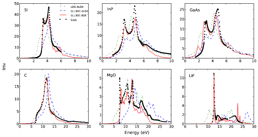
Figure 1: Optical absorption spectra calculated using LDA-ALDA (dash-dotted line), GLLBSC-ALDA (dashed line) as well as GLLBSC-BSE (solid line). The derivative discontinuity, $\Delta_{\mathrm{xc}}$, is included in the GLLBSC calculations. The calculated spectra are compared with experimental data (dots, Ref. Palik, 1985, 1991, 1998).

Compared to LDA band gaps (first column), GLLBSC even without the discontinuity (second column) improves the band gaps. The reason is that the GLLBSC potential Eq. (20) can reproduce the asymptotic $1/r$ behavior of the Coulomb potentialGritsenko et al. (1995) and thus the Kohn-Sham eigenvalues are improved over LDA. By adding the discontinuity (third column), the band gaps agree reasonably well with experimental data (last column). The mean absolute error (MAE) with respect to the experimental data is 0.31 eV in agreement with a previous study using GLLBSC for oxides in the perovskite structureCastelli et al. (2012). The sign of the deviations from experiment seem to vary randomly. This is in contrast to the G₀W₀ results (fourth column), which systematically underestimates the band gaps with the largest error being almost 1 eV. We note that (quasi-) selfconsistent GW calculations have been shown to improve the ionization potentials of moleculesRostgaard et al. (2010) and band gaps of solidsvan Schilfgaarde et al. (2006) by reducing the overscreening resulting from the LDA starting point. However, such calculations are even more computationally demanding than G₀W₀, and are therefore not normally used for the calculation of optical spectra. We will show in the following that GLLBSC represents a cheap alternative means to GW providing not only reasonable fundamental gaps, but also very good optical dielectric constants and absorption spectra.

IV.2 Dielectric constants

Table II shows the calculated static macroscopic dielectric constants. In addition to the parameters presented for obtaining the band gaps, 60 - 90 unoccupied bands, corresponding to around 140 eV above the Fermi level, were used in the calculation of the response function Eq. (II.2). Local field effects were included up to an energy cutoff of 150 - 250 eV, which varies according to the size of the unit cell and corresponds to 169 $\bm{\mathrm{G}}$ vectors. The static dielectric constants obtained using LDA-RPA (first column), that is, RPA calculations based on LDA wave functions and energies, are generally higher than the experimental values (last column) due to the underestimated LDA band gaps. The overestimation is enhanced by inclusion of the ALDA kernel (the second row for each semiconductor), in agreement with previous studiesYan et al. (2011b). The GLLBSC without the discontinuity increase the band gaps relative to LDA and consequently reduces the dielectric function towards the experimental value. The inclusion of the discontinuity further opens up the gap and the corresponding dielectric constants (third column) systematically underestimate the experimental values. This underestimation is a result of the neglect of electron-hole interaction when the response function is evaluated at the RPA and (to some extent) ALDA levels. In order to reduce the error coming from this effect, the response function should be evaluated using ”dressed” single-particle energies rather than the bare QP energies. In the following, we use the GLLBSC(wo.)-RPA dielectric function for calculating $W$.

IV.3 Absorption spectra

The absorption spectra calculated using TDDFT and the BSE are shown in Fig. 1. TDDFT calculations were performed using the ALDA kernel and the same parameters as used for obtaining the dielectric constants (see previous section). For the BSE calculations we used an $8\times 8\times 8$ Monkhorst-Pack $k$-point grid not containing the Gamma-point (for InP $10\times 10\times 10$ $k$-points were used). We have also checked the spectra with $12\times 12\times 12$ $k$-point sampling. The main peaks in the absorption spectra are well converged with the applied $k$-point sampling, however, a complete elimination of the small ”wiggles” seen in the spectra would require significantly denser $k$-point sampling. The screened interaction kernel, $W_{\bm{\mathrm{G}}\bm{\mathrm{G}}^{\prime}}(\bm{\mathrm{q}})$, was obtained using GLLBSC(wo.)-RPA, with 60 unoccupied bands and local field effects included by 169 $\bm{\mathrm{G}}$-vectors. Three valence and three conduction bands were taken into account in constructing the BSE matrix. Again, this is sufficient to converge the major (excitonic) peaks and the low energy part of the absorption spectra. The Tamm-Dancoff approximationOnida et al. (2002), consisting of the neglect of coupling between v-c and c-v transitions, was employed. The effect of temperature, which in general lowers the band gap and smears the absorption spectrumMarini (2008), is not considered in the current work. As a result, the spectra presented here are broadened using smearing factors (in units of eV): Si (0.10), C (0.35), InP (0.20), MgO (0.25), GaAs (0.20) and LiF (0.12).

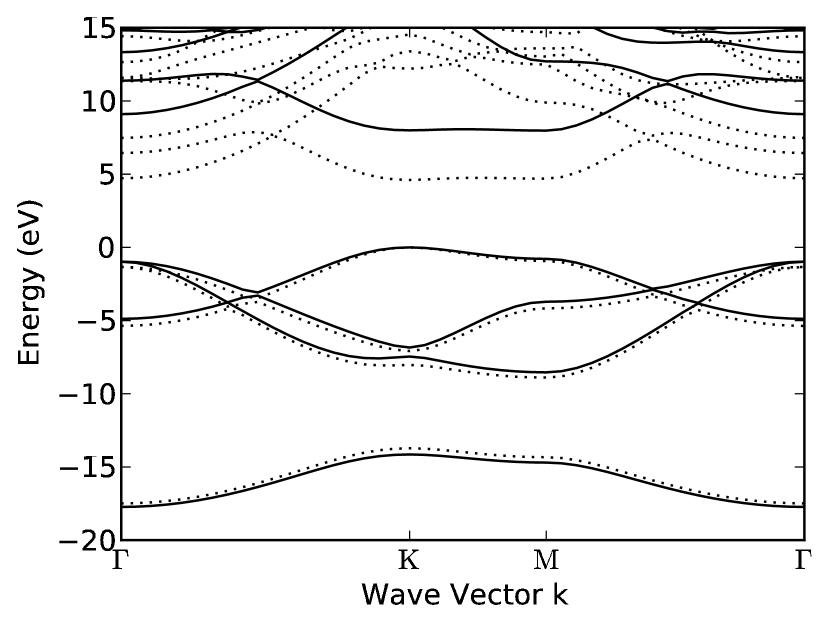
Figure 2: Band structure of a h-BN sheet calculated with GLLBSC (solid lines) and LDA (dotted lines). The top of the valence bands is set to zero.

As can be seen from the absorption spectra in Fig. 1, LDA-ALDA (green dash-dotted lines) gives threshold optical transition energies that are 0.5 - 3 eV lower than experiments (black dots). This is a result of the too low LDA band gaps. The use of GLLBSC wave functions and energies including the derivative discontinuity, GLLBSC-ALDA (blue dashed lines) increases the absorption threshold energies and improves the agreement with experiments. However, the shape of the spectra are qualitalitvely different. In particular, the spectra are too low at the on-set of the absorption and the excitonic features in Si, MgO, and LiF, are completely missed. This is because ALDA does not properly account for electron-hole interactions. In contrast the spectra obtained from the BSE using the GLLBSC eigenvalues as QP energies (red lines) are in excellent agreement with experiments. A small exception is for GaAs where a small peak, abscent in the experimental spectrum, is seen at around 2 eV. A similar feature was seen in a previous calculaton employing a non-local approximation to the xc kernel within TDDFTSharma et al. (2011), but does not appear in a previous GW-BSE calculationArnaud and Alouani (2001). This indicates that the presence of the feature is related to differences between the GLLBSC and GW band structure. We note that (small) deviations between the GLLBSC and GW band structures was recently proposed as the reason for (slight) inaccuracies in the GLLBSC-ALDA calculated surface plasmon energies of Ag(111)Yan et al. (2011a).

V Graphene/boron-nitride

In this section we study the bandstructure and optical absorption spectra of graphene, a single layer of hexagonal boron-nitride (h-BN), and their interface graphene/h-BN. The lattice parameter of h-BN is very similar to that of graphene making it a promising candidate substrate material for graphene based devicesDean et al. (2010). In contrast to graphene, which is a semi-metal, h-BN has a wide band gap and exhibits strong excitonic effects. The optical properties of layered BN sheets as well as BN nanotubes have been studied extensively both experimentallyWatanabe et al. (2004) and theoreticallyArnaud et al. (2006); Wirtz et al. (2006). Upon adsorption of graphene onto a h-BN sheet, a small bandgap of around 10-200 meV, depending on the configuration and interplane distance, emergesGiovannetti et al. (2007). The ground state electronic properties, including the role of dispersive forces, and the band structure have been studiedGiovannetti et al. (2007); Sachs et al. (2011). Below we investigate the optical properties of the graphene/h-BN interface and assess the quality of the GLLBSC for such 2D structure.

Before presenting the results for graphene/h-BN, first we examine a single h-BN sheet. For the lattice constant of h-BN we used 2.89Å and 20Å vacuum was included between the periodically repeated BN layers. Figure 2 shows the band structure calculated using LDA (dotted lines) and GLLBSC (solid lines). The LDA band gap (situated at the K-point) is 4.61 eV which is 0.3 eV larger than reported in an earlier pseudopotential studyBlase et al. (1995). The GLLBSC band gap is 7.99 eV, which includes the derivative discontinuity of 2.12 eV, is close to the pseudopotential G₀W₀ band gap of 7.9 eVWirtz et al. (2006).

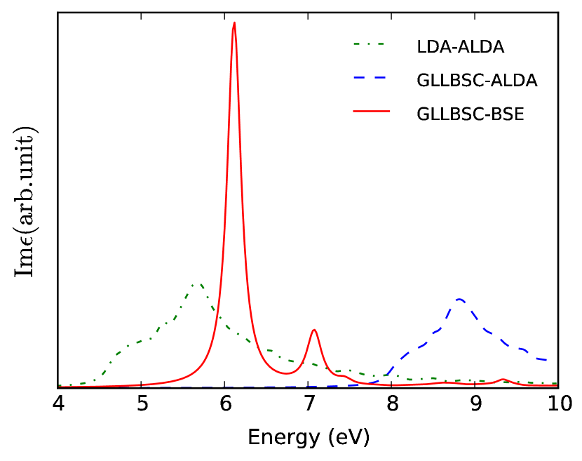
Figure 3: Optical absorption spectra of a h-BN sheet calculated using LDA-ALDA (dash-dotted line), GLLBSC-ALDA (dashed line) and GLLBSC-BSE (solid line).

Figure 3 shows the absorption spectrum of a h-BN sheet obtained with three different methods. The LDA-ALDA spectrum shows a broad absorption peak with an onset at 4.5 eV in good agreement with literatureWirtz et al. (2006). The GLLBSC-ALDA spectrum is essentially identical to LDA-ALDA, but blue shifted by the difference in the band gap. For the BSE calculation, the Brillouin zone was sampled on a non Gamma-centered $32\times 32$ Monkhorst-Pack grid, and 70 unoccupied bands were included to obtain the screened interaction $W$. A two-dimensional Coulomb cutoff techniqueRozzi et al. (2006) was used to avoid interactions between supercells. Since we are interested in the low-energy part of the absorption spectrum and because the valence and conduction bands are well separated from the rest of the bands in the relevant part of the Brillouin zone (around the K-point), only the valence and conduction bands were included in the BSE effective Hamiltonian. The absorption spectrum obtained with GLLBSC-BSE shows three excitonic peaks at 6.1, 7.1 and 7.4 eV with decreasing amplitude. These exciton energies agree well with the value of 6.2 eV, 7.0 eV and 7.4 eV obtained with the GW-BSE schemeWirtz et al. (2006).

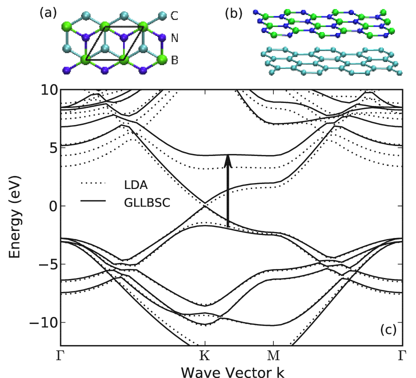
Figure 4: Top (a) and side (b) view of a graphene/h-BN. (c) Band structure of graphene/h-BN calculated with GLLBSC (solid lines) and LDA (dotted lines). The top of the valence bands is set to zero.

For the graphene/h-BN interface, we studied the structure where one C atom is ontop of a B atom and the other C atom is above the center of the BN ring, as shown in Fig. 4 (a) and (b). Both graphene and h-BN are kept planar at a distance 3.48Å apart. Recent RPA calculations found this structure and adsorption distance to be the most stableSachs et al. (2011). Fig. 4 shows the band structure of graphene/h-BN. For the LDA band structure (dotted lines), a small band gap of 31 meV opens at the K point. This number is very close to the 53 meV found in an earlier studyGiovannetti et al. (2007). The h-BN gap, indicated by the arrow and is 4.60 eV in the LDA, which is essentially the same as found for the isolated h-BN sheet (4.61 eV). This is in contrast to the GLLBSC band structure which yields a band gap of the adsorbed h-BN of 6.01 eV which is 1.98 eV lower than obtained for isolated h-BN. This sizable reduction of the gap is not due to hybridization, but rather is a result of a reduction of the derivative discontinuity from 2.12 eV to essentially zero. We note in passing that the GLLBSC value of 6.01 eV is 0.3 eV larger than our G₀W₀ results for this system (to be published elsewhere).

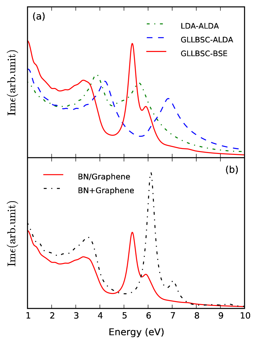
Figure 5: Upper panel: Optical absorption spectrum of graphene/h-BN calculated using LDA-ALDA (dash-dotted line), GLLBSC-ALDA (dashed line) and GLLBSC-BSE (solid line). Lower panel: The GLLBSC-BSE spectrum of the interface (repeated) together with the sum of the absorption spectra of an isolated graphene and BN layer, respectively.

The reduction of the fundamental gap when BN is adsorbed on graphene is physically meaningful and can be explained by the screening provided by the graphene layer (image charge effect) which reduces the energy cost of removing electrons/holes from the BN layer. For molecules on surfaces, this effect has been shown to be well described by the GW method, whereas both (semi-)local and hybrid functionals completely miss the effect predicting no change in the gap upon adsorption (apart from obvious hybridization effects)Neaton et al. (2006); Garcia-Lastra et al. (2009). Interestingly, within the GLLBSC the gap reduction is a result of the vanishing, or strong reduction, of the derivative discontinuity. However, this also has the unphysical consequence that the reduction is present independent of the graphene-BN distance. This follows from the obsrvation that the derivative discontinuity in Eq. (19) becomes zero for a metallic system.

The absorption spectrum of graphene/BN calculated with the three different schemes are shown in Fig. 5(a). Due to the semi-metallic nature of graphene and the dense set of intra band transitions in the 0-5 eV energy region, a much denser k-point sampling is required to obtain a smooth absorption spectrum for this system. We used a $80\times 80$ Monkhorst-Pack grid for both the ALDA and BSE calculations. 70 unoccupied bands were taken into account for the calculation of the response function, while 2 valence and 2 conduction band were included in the BSE Hamiltonian. The energy range below 1 eV is not shown in the figure since the excitations close to the Dirac point requires even denser k-points sampling.

The LDA-ALDA spectrum (dashed-dotted line) shows absorption peaks at 3.9 and 5.6 eV originating from transitions within the graphene and BN layer, respectively. It closely resembles a superposition of the spectra from freestanding graphene (not shown here) and BN sheets (dashed-dotted line in Fig. 3) , with only a minor difference of 0.1 eV in peak positions. Using GLLBSC-ALDA (dashed line), the two peaks shift up to 4.2 and 6.8 eV, respectively. The shift in the BN peak position is in accordance with the shift in the BN gap in Fig. 4. Note that the graphene peak energy of 4.2 eV is much lower than the 5.15 eV obtained from a previous G₀W₀ calculation (without electron-hole interaction)Yang et al. (2009). We speculate that the deviation is due to an incorrect description of the slope of the graphene bands around the Dirac point where GLLBSC yields essentially the LDA result, see Fig. 4. Although the absolute absorption peak for graphene is underestimated, the excitonic effect is still well described using the BSE. With electron-hole pair interaction included (solid line), the graphene absorption peak at 4.2 eV is redshifted by 0.6 eV, the same amount as was found in Ref. Yang et al., 2009. The shift in the BN peak is, however, more striking. Upon adsorption of graphene, the BN exciton peak shifts from 6.1 eV in Fig. 3 to 5.4 eV in Fig. 5. The reduction of the exciton energy of 0.7 eV is much smaller than the 1.98 eV reduction of the fundamental gap. This means that the exciton binding energy has been reduced from 1.9 eV in freestanding BN to 0.6 eV when adsorbed on graphene. Again, this is explained by the enhanced screening of the electron-hole pair provided by the electrons in graphene. The substrate induced screening of exciton binding energies was recently observed in GW-BSE calculations for molecules adsorbed on a metal surface.Garcia-Lastra and Thygesen (2011)

VI Conclusions

We have presented an implementation of the Bethe-Salpeter equation (BSE) which allows for the calculation of optical properties of materials with proper account of electron-hole interactions. Rather than following the standard approach where quasiparticle energies are obtained from the computationally costly GW method, we showed that excellent agreement with experimental absorption spectra of a representative set of semiconductors and insulators, can be obtained by using single-particle energies from the GLLBSC functional. The latter yields very good fundamental gaps due to its explicit inclusion of the derivative discontinuity, and its computational cost is comparable to LDA. For a single layer of boron-nitride the fundamental gap and optical spectrum obtained with GLLBSC-BSE is very close to that of previous GW-BSE calculations. We showed that when BN is adsorbed on graphene, the fundamental gap is reduced by 2 eV. This reduction can be explained by image charge screening, and shows up in the GLLBSC calculation as a vanishing contribution from the derivative discontinuity. Finally, we found that the absoption spectrum of graphene/BN interface is not simply a sum of the absorption spectra of the isolated layers, because the transition energies in BN become redshifted by up to almost 1 eV due to screening by the graphene electrons.

Appendix A Effective two-particle Hamiltonian

To obtain an effective two-particle Hamiltonian describing the optical excitations of the interacting electron system, we begin by considering the Bethe-Salpeter equation (BSE) for the (retarded) four-point response function, $\chi^{\text{4P}}$. Assuming a static electron-hole interaction kernel $\chi^{\text{4P}}$ can be written

$$\chi^{\text{4P}}(\bm{\mathrm{r}}_{1}\bm{\mathrm{r}}_{2};\bm{\mathrm{r}}_{3}\bm{\mathrm{r}}_{4},\omega)=P^{\text{4P}}(\bm{\mathrm{r}}_{1}\bm{\mathrm{r}}_{2};\bm{\mathrm{r}}_{3}\bm{\mathrm{r}}_{4},\omega)+\int P^{\text{4P}}(\bm{\mathrm{r}}_{1}\bm{\mathrm{r}}_{2};\bm{\mathrm{r}}_{5}\bm{\mathrm{r}}_{6},\omega)K^{\text{4P}}(\bm{\mathrm{r}}_{5}\bm{\mathrm{r}}_{6};\bm{\mathrm{r}}_{7}\bm{\mathrm{r}}_{8})\chi^{\text{4P}}(\bm{\mathrm{r}}_{7}\bm{\mathrm{r}}_{8};\bm{\mathrm{r}}_{3}\bm{\mathrm{r}}_{4},\omega)d\bm{\mathrm{r}}_{5}d\bm{\mathrm{r}}_{6}d\bm{\mathrm{r}}_{7}d\bm{\mathrm{r}}_{8}$$ (27)

In writing the above BSE equation we have made the simplifying, and for practical purposes essential, assumption that the electron-hole interaction kernel, $K$, is frequency independent. The quantity $\chi^{\text{4P}}$ is an uncontracted version of the density response function, i.e. $\chi(\bm{\mathrm{r}},\bm{\mathrm{r}}^{\prime},\omega)=\chi^{\text{4P}}(\bm{\mathrm{r}}\bm{\mathrm{r}};\bm{\mathrm{r}}^{\prime}\bm{\mathrm{r}}^{\prime},\omega)$ while $P^{\text{4P}}$ is the four-point response function for independent (but self-energy dressed) quasiparticles (QP). The kernel is given by $K^{\text{4P}}=V-\frac{1}{2}W$ where

$$V(\bm{\mathrm{r}}_{1}\bm{\mathrm{r}}_{2};\bm{\mathrm{r}}_{3}\bm{\mathrm{r}}_{4})=\frac{1}{|\bm{\mathrm{r}}_{1}-\bm{\mathrm{r}}_{3}|}\delta(\bm{\mathrm{r}}_{1}-\bm{\mathrm{r}}_{2})\delta(\bm{\mathrm{r}}_{3}-\bm{\mathrm{r}}_{4})$$ (28)

is the electron-hole exchange and

$$W(\bm{\mathrm{r}}_{1}\bm{\mathrm{r}}_{2};\bm{\mathrm{r}}_{3}\bm{\mathrm{r}}_{4})=\int\frac{\epsilon^{-1}(\bm{\mathrm{r}}_{1},\bm{\mathrm{r}}^{\prime},0)}{|\bm{\mathrm{r}}^{\prime}-\bm{\mathrm{r}}_{2}|}d\bm{\mathrm{r}}^{\prime}\delta(\bm{\mathrm{r}}_{1}-\bm{\mathrm{r}}_{3})\delta(\bm{\mathrm{r}}_{2}-\bm{\mathrm{r}}_{4})$$ (29)

is the statically screened direct electron-hole interaction.

Assuming that the QP energies and wave functions can be described by an effective non-interacting Hamiltonian, $H_{\text{QP}}$, we can write the independent response function as

$$P^{\text{4P}}(\bm{\mathrm{r}}_{1}\bm{\mathrm{r}}_{2};\bm{\mathrm{r}}_{3}\bm{\mathrm{r}}_{4},\omega)=\frac{2}{\Omega}\sum_{\bm{\mathrm{q}}}\sum_{\bm{\mathrm{k}}nm}(f_{n\bm{\mathrm{k}}}-f_{m\bm{\mathrm{k}}+\bm{\mathrm{q}}})$$

$$\times\frac{\psi_{n\bm{\mathrm{k}}}^{\ast}(\bm{\mathrm{r}}_{1})\psi_{m\bm{\mathrm{k}}+\bm{\mathrm{q}}}(\bm{\mathrm{r}}_{2})\psi_{n\bm{\mathrm{k}}}(\bm{\mathrm{r}}_{3})\psi_{m\bm{\mathrm{k}}+\bm{\mathrm{q}}}^{\ast}(\bm{\mathrm{r}}_{4})}{\omega+\epsilon^{\text{QP}}_{n\bm{\mathrm{k}}}-\epsilon^{\text{QP}}_{m\bm{\mathrm{k}}+\bm{\mathrm{q}}}+i\eta}.$$ (30)

where the wave functions form an orthonormal set and the occupation factors are 1 or 0 for occupied and empty states, respectively.

The full four-point response function can also be expanded in the orthonormal basis of single-particle transitions, $\psi_{S}(\bm{\mathrm{r}}_{1},\bm{\mathrm{r}}_{2})=\psi_{n\bm{\mathrm{k}}}^{\ast}(\bm{\mathrm{r}}_{1})\psi_{m\bm{\mathrm{k}}+\bm{\mathrm{q}}}(\bm{\mathrm{r}}_{2})$,

$$\chi^{\text{4P}}(\bm{\mathrm{r}}_{1}\bm{\mathrm{r}}_{2};\bm{\mathrm{r}}_{3}\bm{\mathrm{r}}_{4},\omega)=\sum_{\bm{\mathrm{q}}}\sum_{SS^{\prime}}\chi_{SS^{\prime}}(\bm{\mathrm{q}},\omega)$$ (31)

$$\times\psi_{n\bm{\mathrm{k}}}^{\ast}(\bm{\mathrm{r}}_{1})\psi_{m\bm{\mathrm{k}}+\bm{\mathrm{q}}}(\bm{\mathrm{r}}_{2})\psi_{n^{\prime}\bm{\mathrm{k}}^{\prime}}(\bm{\mathrm{r}}_{3})\psi_{m^{\prime}\bm{\mathrm{k}}^{\prime}+\bm{\mathrm{q}}}^{\ast}(\bm{\mathrm{r}}_{4})$$

As a consequence of the periodicity of the crystal lattice, all 4-point functions are diagonal in $\bm{\mathrm{q}}$. Note that the indices $n,m,n^{\prime},m^{\prime}$ must run over all bands, both occupied and unoccupied, in order to ensure that the two-particle basis is complete (it will, however, turn out that it is sufficient to consider only e-h and h-e transitions).

The non-interacting response function is diagonal in the two-particle basis,

$$P^{\text{4P}}_{SS^{\prime}}(\bm{\mathrm{q}},\omega)=\frac{f_{S}}{\omega-\varepsilon_{S}+i\eta}\delta_{SS^{\prime}}$$ (32)

where the occupation and transition energy for an electron hole pair $S$ is defined as

$$f_{S}\equiv f_{n\bm{\mathrm{k}}}-f_{m\bm{\mathrm{k}}+\bm{\mathrm{q}}}$$ (33)

$$\varepsilon_{S}\equiv\varepsilon_{n\bm{\mathrm{k}}}-\varepsilon_{m\bm{\mathrm{k}}+\bm{\mathrm{q}}}$$ (34)

The four point Bethe-Salpeter equation Eq. (27) in the two-particle basis corresponding to momentum transfer $\bm{\mathrm{q}}$ becomes

$$\chi_{SS^{\prime}}^{4\text{P}}(\bm{\mathrm{q}},\omega) =P^{4\text{P}}_{SS}(\bm{\mathrm{q}},\omega)$$ (35)

$$+\sum_{S^{\prime\prime}}P^{4\text{P}}_{SS}(\bm{\mathrm{q}},\omega)K^{4\text{P}}_{SS^{\prime\prime}}(\bm{\mathrm{q}},\omega)\chi^{4\text{P}}_{S^{\prime\prime}S^{\prime}}(\bm{\mathrm{q}},\omega)$$

Expressions for the kernel matrix elements are given in Eqs. (10) and (II.3).

Substituting Eq. (32) into Eq. (35) and rearranging yields

$$\chi_{SS^{\prime}}^{4\text{P}}(\bm{\mathrm{q}},\omega)=[I(\omega+i\eta)-\mathcal{H}(\bm{\mathrm{q}},\omega)]^{-1}_{SS^{\prime}}f_{S^{\prime}}$$ (36)

where the effective two-particle Hamiltonian, $\mathcal{H}$, is defined as

$$\mathcal{H}_{SS^{\prime}}(\bm{\mathrm{q}},\omega)\equiv\varepsilon_{S}\delta_{SS^{\prime}}+f_{S}K^{4\text{P}}_{SS^{\prime}}(\bm{\mathrm{q}},\omega),$$ (37)

and $I$ is an identity matrix with the same dimension as $\mathcal{H}$.

By dividing the matrices into $4\times 4$ blocks corresponding to two-particle basis functions containing e-h, h-e, e-e, and h-h transitions, it follows that $\chi_{SS^{\prime}}^{4\text{P}}$ is non-zero only within the $2\times 2$ upper left block. For this reason we can reduce the problem by limiting the two-particle basis functions, $\psi_{S}$, to the e-h and h-e states. Using the eigenstates and energies of the BSE Hamiltonian,

$$\mathcal{H}(\bm{\mathrm{q}})A_{\lambda}(\bm{\mathrm{q}})=E_{\lambda}(\bm{\mathrm{q}})A_{\lambda}(\bm{\mathrm{q}})$$ (38)

we can construct the spectral representation of the resolvent of the BSE Hamiltonian,

$$\left[I(\omega+i\eta)-\mathcal{H}(\bm{\mathrm{q}})\right]^{-1}_{SS^{\prime}}=\sum_{\lambda\lambda^{\prime}}\frac{A_{\lambda}^{S}(\bm{\mathrm{q}})[A_{\lambda^{\prime}}^{S^{\prime}}(\bm{\mathrm{q}})]^{\ast}N^{-1}_{\lambda\lambda^{\prime}}(\bm{\mathrm{q}})}{\omega-E_{\lambda}(\bm{\mathrm{q}})+i\eta}$$ (39)

where $N_{\lambda\lambda^{\prime}}(\bm{\mathrm{q}})$ is the overlap matrix defined as

$$N_{\lambda\lambda^{\prime}}(\bm{\mathrm{q}})\equiv\sum_{S}[A_{\lambda}^{S}(\bm{\mathrm{q}})]^{\ast}A_{\lambda^{\prime}}^{S}(\bm{\mathrm{q}})$$ (40)

The BSE Hamiltonian (38) is in general non-Hermitian as a matrix in the e-h and h-e basis. However, within the standard Tamm-Dancoff approximation, in which only the e-h transitions are considered (i.e. transitions with positive energies), $\mathcal{H}(\bm{\mathrm{q}})$ becomes Hermitian and $N_{\lambda\lambda^{\prime}}(\bm{\mathrm{q}})=\delta_{\lambda\lambda^{\prime}}$.

Since the two-point response function, $\chi_{\bm{\mathrm{G}}\bm{\mathrm{G}}^{\prime}}(\bm{\mathrm{q}},\omega)$, is obtained by Fourier transforming $\chi^{\text{4P}}(\bm{\mathrm{r}}\bm{\mathrm{r}};\bm{\mathrm{r}}^{\prime}\bm{\mathrm{r}}^{\prime},\omega)$, we conclude from Eq. (31) that

$$\chi_{\bm{\mathrm{G}}\bm{\mathrm{G}}^{\prime}}(\bm{\mathrm{q}},\omega)=\frac{1}{\Omega}\sum_{SS^{\prime}}\chi^{4\text{P}}_{SS^{\prime}}(\bm{\mathrm{q}},\omega)n_{S}(\bm{\mathrm{G}})n^{\ast}_{S^{\prime}}(\bm{\mathrm{G}}^{\prime})$$ (41)

where the charge density matrix, $n_{S}(\bm{\mathrm{G}})$, is defined in Eq. (5).

Finally, the relation to the macroscopic dielectric function Eq. (16) is established using Eqs. (36) and (39), together with the relation

$$\epsilon(\omega)=1-\frac{4\pi}{|\bm{\mathrm{q}}|^{2}}\bar{\chi}_{00}(\bm{\mathrm{q}}\rightarrow 0,\omega)$$ (42)

between the dielectric function and the irreducible response function, $\bar{\chi}$. As discussed in Sec. II.3 the latter is obtained in place of $\chi$ when the long range $\bm{\mathrm{G}}=0$ term excluded from the e-h exchange kernel in Eq. (10).