Phenomenology of the minimal supersymmetric extension of the standard model
Abstract
We discuss the minimal supersymmetric extension of the standard model. Gauge couplings unify as in the MSSM, even if the scale of breaking is as low as order TeV and the model can be embedded into an grand unified theory. The phenomenology of the model differs in some important aspects from the MSSM, leading potentially to rich phenomenology at the LHC. It predicts more light Higgs states and the mostly left CP-even Higgs has a mass reaching easily 125 GeV, with no constraints on the SUSY spectrum. Right sneutrinos can be the lightest supersymmetric particle, changing all dark matter constraints on SUSY parameter space. The model has seven neutralinos and squark/gluino decay chains involve more complicated cascades than in the MSSM. We also discuss briefly low-energy and accelerator constraints on the model, where the most important limits come from recent searches at the LHC and upper limits on lepton flavour violation.
pacs:
14.60.Pq, 12.60.Jv, 14.80.CpI Introduction
Within the minimal supersymmetric extension of the standard model (MSSM) the gauge couplings unify nearly perfectly around an energy scale of approximately GeV, if SUSY particles exist with masses of the order of TeV. Extending the MSSM with non-singlet superfields tends to destroy this attractive feature, unless (a) the additional fields come in complete multiplets or (b) the standard model gauge group is extended too. Here we study a model in which the SM group is enlarged to . It is a variant of the models first proposed in Malinsky:2005bi and later discussed in more detail in DeRomeri:2011ie .
Our main motivation for studying this model can be summarized as: (i) It unifies, in the same way the MSSM does, even if the scale of breaking is as low as the electro-weak scale; (ii) it can be easily embedded into an grand unified theory; (iii) it has the right ingredients to explain neutrino masses (and angles) by either an inverse Mohapatra:1986bd or a linear Akhmedov:1995vm ; Akhmedov:1995ip seesaw; (iv) it allows for Higgs masses significantly larger than the MSSM without the need for a very heavy SUSY spectrum Hirsch:2011hg and (v) it potentially leads to rich phenomenology at the LHC.
With the data accumulated in 2011 both ATLAS ATLAS:2012ae and CMS Chatrchyan:2012tx have seen some indications for a Higgs boson with a mass of roughly GeV. This result, perhaps unsurprisingly, has triggered an avalanche of papers studying the impact of such a relatively hefty Higgs on the supersymmetric parameter space Hall:2011aa ; Baer:2011ab ; Feng:2011aa ; Heinemeyer:2011aa ; Arbey:2011ab ; Arbey:2011aa ; Draper:2011aa ; Moroi:2011aa ; Carena:2011aa ; Ellwanger:2011aa ; Buchmueller:2011ab ; Akula:2011aa ; Kadastik:2011aa ; Cao:2011sn ; Arvanitaki:2011ck ; Gozdz:2012xx ; Gunion:2012zd ; Ross:2011xv ; Ross:2012nr ; FileviezPerez:2012iw ; Karagiannakis:2012vk ; King:2012is ; Kang:2012tn ; Chang:2012gp ; Aparicio:2012iw ; Roszkowski:2012uf ; Ellis:2012aa ; Baer:2012uy ; Desai:2012qy ; Cao:2012fz ; Maiani:2012ij ; Cheng:2012np ; Christensen:2012ei ; Vasquez:2012hn ; Ellwanger:2012ke . The general consensus seems to be, that the MSSM can generate GeV only if squarks and gluinos have masses in the multi-TeV range. While this is, of course, perfectly consistent with the lower bounds on SUSY masses obtained from / searches at the LHC ATLAS-WEB ; CMS-WEB , such a heavy spectrum could make it quite difficult indeed for the LHC to find direct signals for SUSY.
There are, of course, several possibilities to circumvent this conclusion. First of all, it is well-known that the loop corrections to are dominated by the top quark-squark loops. Thus, little or no constraints on sleptons and on squarks of the first two generations can in fact be derived from Higgs mass measurements, once the assumption of universal boundary conditions for the soft SUSY parameters is abandoned. Second, in the next-to-minimal SSM (NMSSM) the can be heavier than in the MSSM due to the presence of new F-terms from the additional singlet Higgs Ellwanger:2011aa ; Ellwanger:2012ke , especially in models with non-universal boundary conditions for the (soft) Higgs mass terms Gunion:2012zd or in the generalized NMSSM Ross:2011xv ; Ross:2012nr . And, third, in models with an extended gauge group additional -terms contribute to the Higgs mass matrices, relaxing the MSSM upper limit considerably Haber:1986gz ; Drees:1987tp ; Cvetic:1997ky ; Zhang:2008jm ; Ma:2011ea . This latter possibility is the case we have studied in a previous paper Hirsch:2011hg using the minimal models of Malinsky:2005bi . Here, we extend the analysis of Hirsch:2011hg , including both Higgs and SUSY phenomenology.
Due to the extended gauge structure the model necessarily has more Higgses than the MSSM. Near D-flatness of the breaking then results in one additional light Higgs, Hirsch:2011hg . Mixing between the MSSM and enhances the mass of the mostly MSSM Higgs and, potentially, affects its decays. This is reminiscent to the situation in the NMSSM, where an additional light and mostly singlet Higgs state seems to be preferred Ellwanger:2011aa ; Ellwanger:2012ke if the signals found by ATLAS ATLAS:2012ae and CMS Chatrchyan:2012tx are indeed due to a 125 GeV Higgs.
The MSSM-like in our model can have some exotic decays. For example, the will decay to two lighter Higgses, if kinematically possible, although this decay can never be dominant due to constraints coming from LEP. The model also includes right-handed neutrinos with electro-weak scale masses and there is a small but interesting part in parameter space where , where the Higgs decays to two neutrinos. These decays always lead to one light and one heavy neutrino, with the latter decaying promptly to either or . (Mostly right) sneutrinos can be lighter than the , in which case the Higgs can have invisible decays.
The SUSY spectrum of the model is also richer than the MSSM: It has seven neutralinos and nine sneutrino states. These additional sneutrinos can easily be the lightest supersymmetric particle (LSP) and thus change all the constraints on SUSY parameter space, usually derived from the requirement that the neutralino be a good dark matter candidate with the correct relic density Nakamura:2010zzi 111Also for the case of a neutralino LSP, constraints on the SUSY parameter space from dark matter can change in case the right Higgsino is light.. Even though the lightest sneutrino can also be the LSP in the MSSM, direct detection experiments have ruled out this possibility a long time ago Falk:1994es . In SUSY decays, within the MSSM right squarks decay directly to the bino-like neutralino, leading to the standard missing momentum signature of supersymmetry. Due to the extended gauge group, right squarks can decay also to heavier neutralinos, leading to longer decay chains and potentially to multiple lepton edges222Longer SUSY cascades from larger number of neutralino states have also been discussed in Ali:2009md ; Belyaev:2012si .. Decays of the heavier neutralinos also produce Higgses, both the and the appear, with ratios depending on the right higgsino content of the neutralinos in the decay chains.
The rest of this paper is organized as follows. In the next section we discuss the setup of the model, its particle content, superpotential and soft terms and the symmetry breaking. The phenomenologically most interesting mass matrices of the spectrum are given in section III where we also discuss numerical results on the SUSY and Higgs mass eigenstates. Here, we focus on Higgs and slepton/sneutrino masses, which are the phenomenologically most interesting. In section IV we define some benchmark points for the model and discuss their phenomenologically most interesting decay chains. We then close with a short summary. In the appendix we give mass matrices not presented in the text, formulas for the 1-loop corrections in the Higgs sector and more information about the calculation of the RGEs, including anomalous dimensions as well as the 1-loop functions for gauge couplings and gauginos.
II The model:
In this section we present the particle content of the model, its superpotential and discuss the symmetry breaking. We consider the simplest model based on the gauge group . We will call this the mBLR model below. As has been shown in Malinsky:2005bi it can emerge as the low-energy limit of a certain class of GUTs broken along the “minimal” left-right symmetric chain
The main virtue of this setting is that an MSSM-like gauge coupling unification is achieved with a sliding breaking scale, i.e. this last stage can stretch down even to the electro-weak scale. Different from the previous works Malinsky:2005bi ; DeRomeri:2011ie , we assume that the first two breaking steps down to happen both at (or sufficiently close to) the GUT scale. This assumption is used only for simplifying our setup, it does not lead to any interesting changes in phenomenology.
II.1 Particle content, superpotential and soft terms
| Superfield | Generations | ||
| 3 | |||
| 3 | |||
| 3 | |||
| 3 | |||
| 3 | |||
| 3 | |||
| 3 | |||
| 1 | |||
| 1 | |||
| 1 | |||
| 1 |
The transformation properties of all matter and Higgs superfields of the model are summarized in table 1. Apart from the MSSM fields, in the matter sector we have and . The former are necessary in the extended gauge group for anomaly cancellation,333 is automatically part of the theory due to its origin. while the fields are included to explain neutrino masses by either an inverse Mohapatra:1986bd or a linear Akhmedov:1995vm ; Akhmedov:1995ip seesaw mechanism. Our Higgs sector, including the new fields and , is the minimal one for the breaking of to .
The fields and can be viewed as the (electric charge neutral) remnants of doublets, which remain light in the spectrum when the gauge factor is broken by the vev of a neutral triplet down to the Malinsky:2005bi . The presence of and makes it necessary to introduce an extra matter parity, since otherwise -parity is broken in a potentially disastrous way, once these scalars acquire vacuum expectation values. This is not a particular feature of our setup; it is always needed in models where is broken with doublets Martin:1992mq . 444In the normalization of Martin:1992mq doublets have , i.e are “odd” under B-L.
The relevant -parity and conserving superpotential is given by
| (2) |
Here,
| (3) | |||||
where , and are the usual MSSM Yukawa couplings for the charged leptons and the quarks. In addition there are the neutrino Yukawa couplings and ; the latter mixes the fields with the fields giving rise to heavy SM-singlet pseudo-Dirac mass eigenstates. The term is completely analogous to the MSSM term. Note that the term is included to generate non-zero neutrino mass with an inverse seesaw mechanism. However, as always is done in inverse seesaw, we assume that is much smaller than all other dimensionful parameters of the model. Apart from neutrino masses themselves it will therefore not affect any of the mass matrices (or decays) of our interest.
Note that, besides the role it plays in neutrino physics, the coupling is relevant also for the Higgs phenomenology at the loop level as it enters the mixing of and Higgs fields with the Higgs doublets as well as the RGEs for , see below.
Following the notation and conventions of Allanach:2008qq the soft SUSY breaking Lagrangian reads
| (4) | |||||
The first sum contains the scalar masses squared and the second sum runs over all gauginos for the different gauge groups (called , , and in the following) and the second one contains the scalar masses squared. While is in principle a free parameter, a naive order of magnitude expectation for it is . Thus, one expects that is much smaller than all other soft terms and can be safely neglected, see discussion of sneutrinos below.
To reduce the number of free parameters, in our numerical studies we will consider a scenario motivated by minimal supergravity. This means that we assume a GUT unification of all soft-breaking sfermion masses as well as a unification of all gaugino mass parameters
| (5) | |||
Also, for the trilinear soft-breaking coupling, the ordinary mSugra conditions are assumed
| (6) |
The GUT scale is chosen as the unification scale of , and , while we allow to be slightly different, exactly as in the MSSM. A complete unification is assumed to happen due to GUT threshold corrections. For the remaining soft parameters in the Higgs sector, , , , and and , we have implemented two different options. These are discussed in section II.2.
The presence of two Abelian groups gives rise to gauge kinetic mixing
| (7) |
This is allowed by gauge and Lorentz invariance Holdom:1985ag , as and are gauge invariant, see e.g. Babu:1997st . Even if and are orthogonal in the kinetic mixing term will be induced during the RGE running below the breaking scale because the light fields remaining below the GUT scale can’t be arranged in complete multiplets: while all matter fields form three generations of 16-plets, and induce off-diagonal elements already in the 1-loop matrix of the anomalous dimensions defined by . The matrix reads
| (8) |
contains the GUT normalization of the two Abelian gauge groups. Our implementation follows the description of Fonseca:2011vn , where it is shown that terms of the form as in eq. (7) can be absorbed in the covariant derivative by a re-definition of the gauge fields. Therefore, we are going to work in the following with covariant derivatives of the form
| (9) |
where is a vector containing the charges of the field with respect to the two Abelian gauge groups and is the gauge coupling matrix
| (10) |
contains the gauge bosons . Since the off-diagonal elements in eq. (8) are negative and roughly one order smaller than the diagonal ones, it can be expected that the off-diagonal gauge couplings at the SUSY scale are positive but also much smaller than the diagonal ones. This is in some contrast to models in which kinetic mixing arises due to the presence of O'Leary:2011yq . In addition, a mixing term of the form
| (11) |
between the two gaugino and will be present Braam:2011xh . Since we have chosen the breaking scale to be very close to the GUT scale we demand as additional boundary conditions that the new parameters arising from kinetic mixing vanish at the GUT scale, i.e.
| (12) |
For more details on mixing and its physical impact we refer the interested reader also to recent papers Chun:2010ve ; Mambrini:2011dw ; O'Leary:2011yq ; Rizzo:2012rf . Our focus will be on the additional terms in the scalar mass matrices due to the presence of non-diagonal couplings.
II.2 Tadpole equations and boundary conditions
The gauge symmetry is spontaneously broken to the hypercharge by the vevs and of the scalar components of the and superfields while the is governed by the vevs and of the neutral scalar components of the Higgs doublets and up to gauge kinetic mixing effects. One can write
| (13) | |||||
| (14) |
where the generic symbols and denote the CP-even and CP-odd components of the relevant fields, respectively.
The minimum conditions for the four different vevs can be written at tree-level as
| (15) | |||
| (16) | |||
| (17) | |||
| (18) |
where we defined
| (19) |
For the vacuum expectation values we use the following parameterization:
| (20) | |||
The tadpole equations can analytically be solved for either (i) (, ) or (ii) (, , ) or (iii) (, , , ). Option (i) can be considered the minimal version. We call this option CmBLR (constrained mBLR), since it allows to define boundary conditions for all scalar soft masses, and at , reducing the number of free parameters by four. This assumption, however, leads to some important constraints on the parameter space, as we will discuss next. Options (ii) and (iii) are more flexible. Option (ii) is similar to the CMSSM with non-universal soft masses (NUHM) Matalliotakis:1994ft ; Polonsky:1994rz ; Berezinsky:1995cj , albeit the non-universality is only in the sector. We will call this the mBLR (non-universal masses mBLR), and most of our numerical results are based on this option. We mention option (iii) for completeness, but we have not used it in our numerical studies.
As will be shown in section III.1, the mass of the -boson in the mBLR model is approximately given by
| (21) |
We can use this expression and eqs (15)-(18) to obtain an approximate relation between and , , and . This leads to
| (22) |
where . We can roughly estimate , if we make a mSugra-like assumption for the boundary conditions, at the GUT scale. The running value of can then be found by a one-step integration of the RGEs at 1-loop level as:
| (23) |
with . As eq.(23) shows, with these assumptions and the condition that of eq.(22) has to fulfill the experimental lower bound will define an excluded area in the 3-dimensional parameter space [, ], where . If we assume in addition that is small enough to remain perturbative anywhere between the weak and the GUT scale, a lower bound on as a function of will result in the CmBLR.
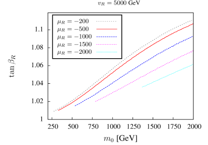
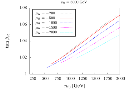
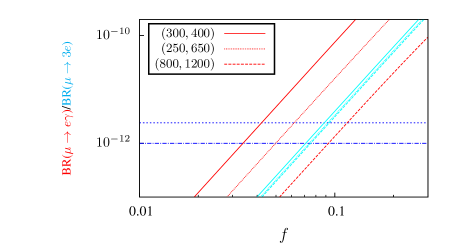
This can be understood in more details as follows. In the CmBLR , as shown by eq. (23) and the last term in eq. (22) is positive only if . Since the second term in eq. (22) is positive only if . If , only solutions with can be found. Since finally must be and in the CmBLR we get the constraints on the parameter space shown in fig. 1. Here we show for two choices of contour lines of in the plane . Just above the lines for GeV , i.e. larger values of do not lead to consistent solutions of the tadpole equations (for fixed and ). This restricts the model to values of very close to , as is clearly demonstrated in the figure. Note that for low values of the constraints on the viable region of actually becomes stronger. 555 is also needed for a spectrum without tachyons since the additional D-terms can give large negative contributions to the sfermion masses, see below.
|
|
No such constraint on and exists in the mBLR, since here is a free parameter. However, if , values of very close to are preferred by eq. (22) in both, the CmBLR and the mBLR.
III Masses
In this section we give the most important mass matrices of the model at tree-level. In the numerical calculations we take also the 1-loop corrections Pierce:1996zz into account, see appendix for more details. The numerical implementation of the model has been done using SPheno Porod:2003um ; Porod:2011nf , for which the necessary subroutines and input files were generated using the package SARAH Staub:2008uz ; Staub:2009bi ; Staub:2010jh . The used model files are included in the public version 3.1.0 of SARAH.
III.1 Gauge bosons
In the basis () the mass matrix for the neutral gauge bosons reads at tree-level
| (24) |
where
| (25) |
From eq. (24) the masses of the photon, the and the can be calculated analytically
| (26) |
with
Expanding eq. 26 in powers of , we find up to first order
| (28) |
In the limit and we then get
| (29) |
ATLAS has recently published updated lower limits on searches ATLAS-CONF-2012-007 . Our corresponds to the in the notation of Erler:2011ud , i.e. ATLAS-CONF-2012-007 gives a lower limit of TeV, which corresponds to roughly TeV for our choice of couplings666The condition that the gauge couplings reproduce correctly the standard model hypercharge, plus the assumption of unification lead to values of roughly , , and at the SUSY scale., see, however, the discussion in section IV.3.
III.2 Higgs bosons
III.2.1 Pseudoscalar Higgs bosons
At the tree level we find that in the basis the pseudoscalar sector has a block-diagonal form and reads in Landau gauge
| (32) |
with
| (37) |
From these four states two are Goldstone bosons which become the longitudinal parts of the massive neutral vector bosons and a . In the physical spectrum there are two pseudoscalars and with masses
| (38) |
III.2.2 Scalar Higgs bosons
The tree-level CP-even Higgs mass matrix in the basis reads
| (41) |
where
| (44) | |||||
| (47) | |||||
| (50) |
, (), , . The matrix contains the standard MSSM doublet mass matrix. To see this explicitly one has to integrate out the additional Higgs fields in the limit which yields a shift in the gauge couplings such that the MSSM limit is achieved. corresponds to the Higgs bosons and provides the essential mixing between the two sectors.
Note that it is straightforward to show that the determinant of the mass matrix eq. (41) goes to zero, whenever one of the parameters () goes to zero. One can also calculate analytically that in the limit of the lightest eigenvalue of eq. (41) obeys the MSSM tree-level limit for . For finite corrections to appear, of the order of , which lead to a shift in the lightest eigenvalue. Thus the MSSM tree-level upper bound of for the lightest Higgs can be violated.
III.2.3 Numerical examples
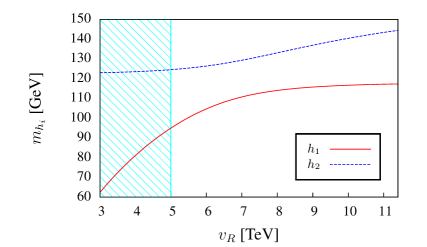
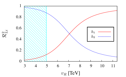
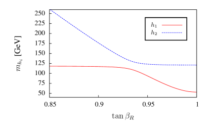
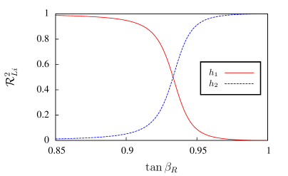
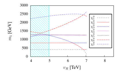
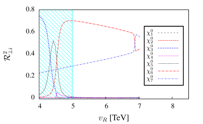
In fig. 2 we show the two lightest Higgs boson masses (to the left) together with
| (51) |
(to the right) as a function of . Here labels the light Higgs scalars in the model and is the rotation matrix which diagonalizes the CP-even Higgs sector. Note that the quantity , which reaches one in the MSSM limit, is a rough measure of how much the corresponding Higgs with index resembles an MSSM Higgs boson. We will call this leftness. Roughly speaking, the smaller this quantities is, the smaller is the -th Higgs coupling to the - and -bosons, implying a reduced production cross sections at LEP, Tevatron and the LHC.
Since the MSSM Higgs and the two additional Higgs and are both charged under the two lightest Higgs states mix due to additional D-terms in the CP-even Higgs matrix (see eq. (44)). Thus, both the masses and the mixing of the two lightest Higgs and depend strongly on , see fig. 2. In this example, up to approximately =6 TeV is mostly the singlet Higgs whereas is the MSSM-like Higgs. For larger a level-crossing occurs and the situation is reversed. Note that, although , and have rather moderate values in this example, has a mass of the order of GeV for TeV, i.e. the D-terms have shifted the MSSM-like Higgs mass into the region preferred by ATLAS and CMS.
|
|
|
|
|
|
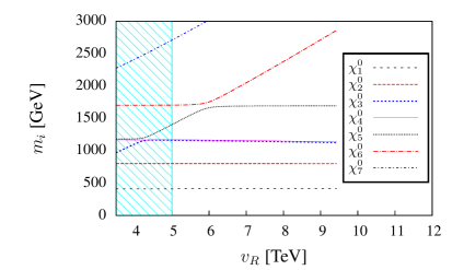
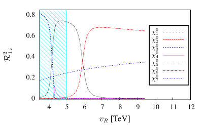
In fig. 3 masses and “leftness” of the two lightest Higgs eigenstates are plotted against . For close to one gets a very light singlet Higgs as expected, see discussion above. As is the case when varying a level-crossing appears also when is changed. In this figure the mBLR version was used, thus we can put . Note, however, that the masses of and show a behavior which is symmetric with respect to . Again the figure demonstrates that the MSSM limit of the lightest Higgs mass can be violated at the expense of a reduced coupling of the MSSM-like state to SM gauge bosons.
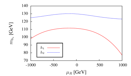
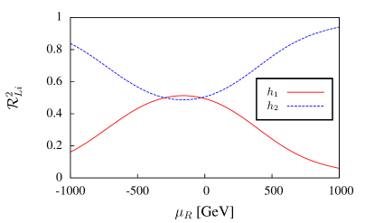
1-loop corrections play in general an important role, not only for the MSSM-like Higgs but also in the singlet sector. This can be seen in fig. 4, where we plot masses and mixings of and versus the parameter . Increasing or decreasing , respectively, changes the mass of the mostly-singlet Higgs by considerable factors. In fact, for larger values of one can get easily a negative mass squared for , which is of course forbidden phenomenologically. The importance of stems from 1-loop contributions to the Higgs mass matrix with a higgsino-right in the loop. Loop corrections for the mostly-singlet Higgs are, in fact, even more important numerically than for the MSSM-like Higgs and many points which are allowed at tree-level lead to tachyonic states, once 1-loop corrections are taken into account.
Finally we note, that in the plots in this section we have not shown the regions excluded by LEP or the LHC searches, since we were interested only in showing the parameter dependencies of our numerical results. In the study points of the next section, however, we have taken care that our points survive all known experimental constraints.
III.3 Neutrinos
The mBLR model contains beside the usual three left-handed neutrinos six additional states which are singlets with respect to the SM group. The corresponding mass matrix is in the basis given by
| (52) |
This matrix is diagonalized by :
| (53) |
Eigenvalues for the three light (and mostly left-handed) neutrinos can be found in the seesaw approximation as:
| (54) |
Neutrino data implies that either and/or is small and in inverse seesaw the smallness of neutrino mass is attributed to the smallness of the latter. As we will discuss in section IV.1, the bounds on rare lepton decays imply that the off-diagonal terms of and have to be small compared to their diagonal entries, unless their diagonal values are small too.
The smallness of implies that the six heavy states form three “quasi-Dirac” pairs. For vanishing off-diagonal entries in and a good estimate of the masses of the heavy states is:
| (55) |
III.4 Sparticles
III.4.1 Neutralinos
The mass matrix of the neutralinos reads in the basis :
| (63) |
The eigenvalues of this matrix are not completely arbitrary. Since is broken in such a way as to produce correctly the SM group in the limit of the matrix contains one state which corresponds to the MSSM bino, , which is a superposition of and . In addition the matrix contains an orthogonal state, which we will call in the following.
For CMSSM like boundary conditions, , the bino is usually the lightest of the three gaugino like states, with the being approximately twice as heavy. The is very often mixed with one of the right higgsinos, and, since at low energies is much smaller than this mixing is often important. In addition, there is the standard quasi-Dirac pair of “left” higgsinos, plus two more states which are mostly right higgsinos. Of the latter one is usually rather heavy, while the other can be light, if is small.
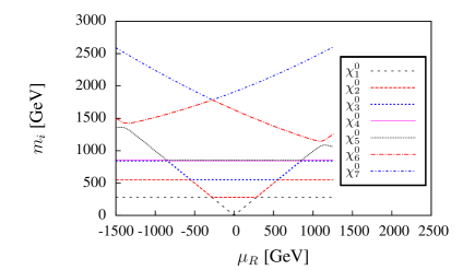
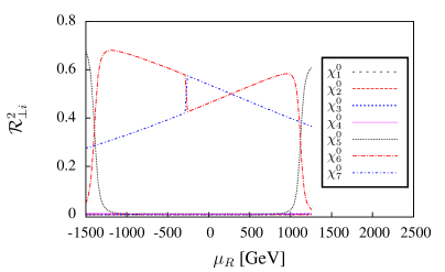
In fig. 5 the neutralino masses and for CmBLR are plotted against for some arbitrary choice of other parameters. As discussed, there are in total seven eigenstates. Of special interest is the , so in the plot on the right we show the percentage of () in the corresponding mass eigenstate. Here means that the -th neutralino is a pure . As one can see in fig. 6 the masses and mixing of the three new states depend strongly on . For small all three states mix to each other. Increasing leads to a decoupling of the lighter higgsino-right from the which decreases in mass since becomes smaller for large while the masses of the two remaining states get large. Since the MSSM Neutralinos mix very little with the new states, there are four eigenvalues which show almost no dependence on the parameters and .
In fig. 6 the neutralino masses and are plotted against for the case of mBLR. In this calculation, and can take fixed values while is varied freely. Two of the three new Neutralino states are a mixture of the higgsino-right and and therefore depend on . Since the lighter higgsino-right hardly mix to the it has a constant mass at GeV in this example. The lighter of the two new states that show dependence on is mostly a , whereas the one with larger mass is mostly a higgsino-right. The smaller the smaller the mixing between these two states and thus the larger the coupling of the mostly -state to the MSSM particles. This will be important when we discuss LHC phenomenology in section IV.5.
The dependence of the neutralino masses and on is shown in fig. 7. Since the higgsino-right and the mix, all three states show a dependence on . The state which hardly mixes to the decreases in mass for small . So we can easily have a higgsino-right as LSP choosing close to zero. The state which is mostly the gets a smaller mass for large , while the one which is mostly a higgsino-right increases in mass.
|
|
|
|
|
|
III.4.2 Sleptons and sneutrinos
In models in which lepton number is broken, the scalar neutrinos split into a real and an imaginary part with slightly different masses Hirsch:1997vz . Since we assume that the smallness of neutrino masses is due to the smallness of the parameter (and, therefore, is supposed to be small too), this splitting between sneutrino mass eigenstates is too small to be of any relevance, except neutrino masses themselves.
Neglecting and the sneutrino mass matrix is given by
| (67) |
where
| (68) |
For charged sleptons one gets:
| (71) |
where
| (72) |
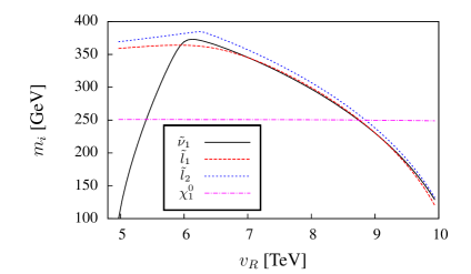
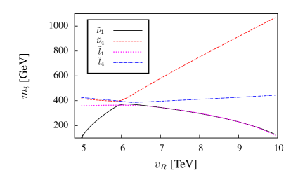
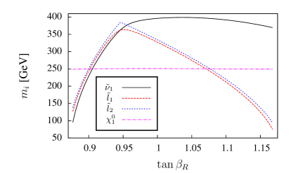
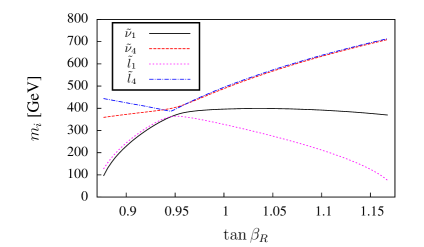
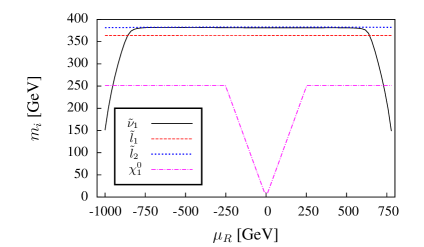
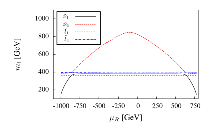
In fig. 8 sneutrino and slepton masses are plotted against , and . The figures on the left show a zoom into the region of the lightest states, whereas the figures on the right show a larger range of masses for a better understanding of the overall behavior. To see which particle is the LSP, while varying , and , we included in all plots on the left the mass of the lightest neutralino state. This state is always a Bino, except for the plot against . Here the LSP becomes a higgsino-right for GeV. The plots show that the masses depend strongly on the choice of and . In the case of charged sleptons the dependence on and comes only from additional D-terms at the tree level. This is different for sneutrinos. Here we can have an interplay between new D-terms and terms coming from the coupling which both depend on and . The additional D-terms force left sparticle to become light for while for right sparticle masses decrease. Up to TeV is a right handed sneutrino and therefore the mass increase for increasing . For TeV the mass of drops down again since here it is mainly a left handed sneutrino. Thus, increasing leads to a level-crossing in the mass spectrum of left and right handed sneutrinos. The same holds for the sleptons. In the plot against the mass of the right sneutrino decreases much faster for TeV than the mass of the right sleptons. This is due to the off-diagonal terms proportional to , which contain also in the sneutrino mass matrix. These terms mix the scalar component of to . Thus for low values of in this example the LSP is neutral, which is allowed, whereas for larger values of (with left sleptons being light) there are parts of the parameter space, where the lightest slepton is charged, which is phenomenologically forbidden. Whether in the left sector charged or neutral states are lighter, depends heavily on the choice of parameters.
Varying the right slepton masses decrease faster than the right sneutrino masses for due the additional sneutrino mixing. Since the sneutrino and slepton masses depend strongly on the choice of , and one obtains limits on combination on these parameters. On the one hand, one has to avoid tachyonic states and on the other hand one has to take care not to get charged sleptons as LSP. The combination of both conditions forces us to choose close to one and gives us an upper limit on and as function of .
|
|
|
|
|
|
IV Constraints, sample spectra and decays
In this section we discuss several interesting phenomenological aspects which potentially allow the BLR model to be discriminated from the MSSM at the LHC and exemplify the most important features for a few study points. We include a discussion of the direct production of new states and characteristic changes in the cascade decays of supersymmetric particles.
For brevity we will call these benchmark points BLRSP1- BLRSP5, the corresponding input parameters are listed in table 2. All of these points have been calculated with the mBLR version of the model. However, note that for BLRSP5 the input is chosen to be consistent with the CmBLR variant.
A few comments on the input parameters and the resulting mass spectra are in order, before we discuss the phenomenology in detail. As shown below, the bounds on rare lepton flavour violating decays require and to be essentially flavour-diagonal, unless these couplings are very small. Therefore we have chosen and diagonal as starting point implying that all points satisfy trivially the LFV constraints. A correct explanation for the neutrino angles then requires flavour violating entries in the parameter , which we do not give in table 2, since they are irrelevant for collider phenomenology.
| BLRSP1 | BLRSP2 | BLRSP3 | BLRSP4 | BLRSP5 | |
| cMSSM | |||||
| [GeV] | 470 | 1000 | 120 | 165 | 500 |
| [GeV] | 700 | 1000 | 780 | 700 | 850 |
| 20 | 10 | 10 | 10 | 10 | |
| 0 | -3000 | -300 | 0 | -600 | |
| Extended gauge sector | |||||
| [GeV] | 4700 | 6000 | 6000 | 5400 | 5000 |
| 1.05 | 1.025 | 0.85 | 1.06 | 1.023 | |
| [GeV] | -1650 | -780 | -1270 | 260 | (-905) |
| [GeV] | 4800 | 7600 | 800 | 2350 | (1482) |
| Yukawas | |||||
| 0.04 | 0.1 | 0.1 | 0.1 | 0.1 | |
| 0.04 | 0.1 | 0.1 | 0.1 | 0.1 | |
| 0.04 | 0.1 | 0.1 | 0.1 | 0.1 | |
| 0.04 | 0.042 | 0.3 | 0.3 | 0.3 | |
| 0.05 | 0.042 | 0.3 | 0.3 | 0.3 | |
| 0.05 | 0.042 | 0.3 | 0.3 | 0.3 | |
The input values of table 2 lead to the mass spectrum shown in table 3. We give the masses and in brackets the particle character. In case of mixed states the two largest components, for example (), are given where the first entry accounts for the larger contribution. If the ordering in the composition changes like in the case of we use squared brackets. Therefore we have for and for . In all cases input parameters have been chosen such, that the squark and gluino masses are outside the region currently excluded by pure CMSSM searches at ATLAS ATLAS-WEB and CMS CMS-WEB . Since (a) we expect the missing momentum signal to be smaller in these points than in a true CMSSM spectrum and (b) our squark spectra are less degenerate than the CMSSM case, we believe this is a conservative choice. Two of the points have a sneutrino LSP (BLRSP1 and BLRSP3), while three points have a neutralino LSP (for BLRSP2 and BLRSP5 mostly a bino, for BLRSP4 a state which is mostly a ).
| BLRSP1 | BLRSP2 | BLRSP3 | BLRSP4 | BLRSP5 | |
| Sneutrinos and Sleptons | |||||
| [GeV] | 102.3 | 797.0 | 91.6 | 542.3 | 753.4 |
| [GeV] | 102.3 | 797.0 | 92.6 | 542.3 | 753.9 |
| [GeV] | 203.0 | 797.0 | 92.6 | 542.3 | 753.9 |
| [GeV] | 573.8 | 1120.1 | 253.4 | 585.4 | 785.5 |
| [GeV] | 604.4 | 1120.3 | 258.2 | 586.7 | 789.0 |
| [GeV] | 725.2 | 1220.0 | 1374.0 | 953.4 | 950.1 |
| [GeV] | 734.1 | 1236.6 | 1374.0 | 953.4 | 950.1 |
| [GeV] | 484.1 | 1013.9 | 254.7 | 263.0 | 580.4 |
| [GeV] | 512.7 | 1055.3 | 265.6 | 270.5 | 592.3 |
| [GeV] | 732.1 | 1222.4 | 447.7 | 591.6 | 788.0 |
| [GeV] | 738.8 | 1237.9 | 450.6 | 592.2 | 790.9 |
| Squarks | |||||
| [GeV] | 1144.0 | 1185.4 | 1247.0 | 1111.3 | 1316.0 |
| [GeV] | 1392.1 | 1851.9 | 1526.9 | 1361.4 | 1643.2 |
| [GeV] | 1456.0 | 2154.7 | 1565.9 | 1392.4 | 1728.0 |
| [GeV] | 1509.0 | 2227.3 | 1634.0 | 1448.8 | 1795.8 |
| [GeV] | 1359.2 | 1819.2 | 1409.8 | 1326.3 | 1611.8 |
| [GeV] | 1464.0 | 2148.1 | 1462.3 | 1420.1 | 1724.5 |
| [GeV] | 1489.8 | 2175.9 | 1462.3 | 1426.2 | 1734.8 |
| [GeV] | 1489.8 | 2175.9 | 1496.2 | 1426.2 | 1734.8 |
| [GeV] | 1509.0 | 2228.9 | 1635.9 | 1450.9 | 1795.8 |
| Higgs (1-loop/2-loop) | |||||
| [GeV] | 59.1/59.6 | 119.2/125.4 | 92.7/93.1 | 100.8/102.6 | 18.8/18.8 |
| [GeV] | 119.0/124.1 | 139.7/140.4 | 114.5/120.1 | 121.0/124.8 | 115.7/121.8 |
| 0.05/0.04 | 0.90/0.83 | 0.07/0.04 | 0.33/0.22 | 0.001/0.001 | |
| 0.95/0.96 | 0.10/0.17 | 0.93/0.96 | 0.67/0.78 | 0.999/0.999 | |
| Neutralinos | |||||
| [GeV] | 282.2 | 416.7 | 312.9 | 258.5 | 346.6 |
| [GeV] | 552.3 | 780.0 | 615.3 | 279.7 | 679.5 |
| [GeV] | 828.9 | 817.5 | 1086.6 | 549.0 | 902.7 |
| [GeV] | 838.9 | 1865.5 | 1092.8 | 844.9 | 1133.1 |
| [GeV] | 1230.4 | 1865.7 | 1232.2 | 856.8 | 1139.4 |
| [GeV] | 1650.9 | 2017.6 | 1811.3 | 1639.0 | 1489.8 |
| [GeV] | 2608.3 | 2392.3 | 2741.4 | 2174.6 | 2056.5 |
Note that the ordering of sfermion mass eigenstates does in many cases not follow the standard CMSSM patterns: and (similar for sdowns). These patterns are distorted in the study points due to the unconventional D-terms of the model and this feature gets enhanced for larger and/or larger values of . We note also that for sneutrinos and charged sleptons many states are quite degenerate. For example and have practically the same mass in all points. While these degeneracies are always true in CMSSM spectra, in our case this is not necessarily so, but simply reflects the fact that both and have been chosen generation independent in all points, except BLRSP1. As this point shows, even a rather moderate generation dependent value of can lead to large mass splittings in the sneutrino sector. A generation dependent value of would not only split sneutrino masses but also charged slepton masses.
IV.1 Lepton decays and LFV
To explain the measured neutrino mixing angles by the mass matrix given in eq. (52) the Yukawa couplings , and/or the the bilinear term have to contain off-diagonal elements. In case that the neutrino mixing is explained by the form of or also lepton flavor violation in the charged lepton sector will be induced. On the one hand the contributions of to the RGE evaluation branching ratios of and to the soft-breaking terms in the lepton sector open decay channels like and similarly to high-scale seesaw type I–III Hirsch:2008dy ; Hirsch:2008gh ; Esteves:2010ff . On the other hand, in inverse seesaw the entries of can be potential large and the dominant contributions to LFV decays can come from diagrams which are proportional to . For a long time it has been assumed that the most stringent bounds on come from the radiative decay while the photonic contributions to are always smaller and therefore must hold. However, recently it has been pointed out that in presence of new Yukawa couplings like the -penguin contributions to can dominate Hirsch:2012ax . These are less suppressed then the photonic contributions by a factor . As consequence, the experimental limits on the decay into two charged electrons can be much more constraining than the radiative decay in case of a heavy SUSY spectrum. We can see this by parametrizing the neutrino Yukawa coupling as
| (73) |
with
| (74) |
Here, and are the mass differences measured in solar and athmospheric neutrino oscillations. The value of accommodates for .
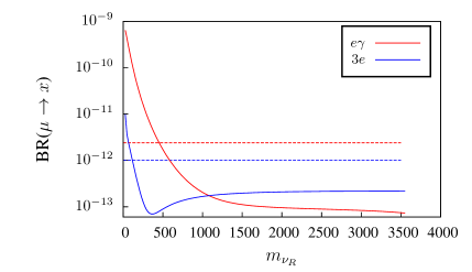
and as function of are depicted in fig. 9, and we show also the most recent, experimental limits of Adam:2011ch ; Nakamura:2010zzi
| (75) |
For the plot we chose three different points for (, ). Since hardly depends on SUSY masses for all three lines lie very close together in contrast to . For light SUSY spectra is dominant whereas the heavier the SUSY particles the more important gets Br(). As shown in BLRSP1 and BLRSP2 we can have light right-handed neutrinos such that contributions from the -graph to LFV can not be neglected anymore. In fig. 10 and are plotted as a function of . For masses below 300 GeV contributions from right-handed neutrinos start to dominate. The minimum in comes from a cancelation between the right-handed neutrino and the corresponding SUSY graph. In the limit of large and converge to the value coming from SUSY contributions.
However, it is possible to circumvent these bounds by assuming that and are diagonal and the entire neutrino mixing is explained by . Of course, this will not only reduce but also .
|
|
IV.2 Higgs physics, direct production
In all study points of table 2 there is one Higgs boson with mass between 120 and 125 GeV. In addition, there is a second state with masses varying between 19 and 140 GeV. In BLRSP1, BLRSP3 and BLRSP5 the mass eigenstate is SM-like, with . In BLRSP2 it is , which has a large content of and and BLRSP4 is a case where and have large mixing. Since we have often a mass eigenstate below the LEP limit of 115 GeV for a standard model Higgs boson, we have checked the consistency of these eigenstates with data using HiggsBounds 3.4.0beta Bechtle:2008jh ; Bechtle:2011sb . All points are allowed by accelerator constraints, but sometimes very close to existing bounds, especially BLRSP4 and also BLRSP2. As an indication for the theoretical uncertainties in the mass calculation we give the masses using the complete 1-loop formulas and the ones adding the dominant 2-loop corrections to the MSSM sector Degrassi:2001yf ; Brignole:2001jy ; Brignole:2002bz ; Dedes:2002dy ; Dedes:2003km ; Allanach:2004rh .
In BLRSP1 and BLRSP5 is so light that the decay is kinematically allowed. However, the mixing between both sectors is so small that for BLRSP1 the corresponding branching ratio is about 1 per-cent whereas for BLRSP5 it is a few per-mile. The smallness of this decay is a direct consequence of the bounds imposed by LEP and the decay can never be dominant in the BLR model. The can also decay into a combination of heavy and light neutrinos with a branching ratio of a few per-cent, as for example in case of BLRSP1 leading to the final states
| (76) | |||||
| (77) |
with and . These final states can also be obtained via intermediate states containing an off-shell vector boson, e.g. and . However, their existence implies that ratio of quark versus lepton final states will not correspond to the branching ratios of the vector bosons. Note, however, that for hadronic W-boson decays the invariant mass of +lepton system would show a peak at the heavy neutrino mass, which allows to identify this signature, in principle. Apart from these decays, the can also decay to two scalar neutrinos and, if kinematically allowed, this decay can become dominant, leading to a (nearly) invisible Higgs boson.
The hint for a 125 GeV Higgs boson ATLAS:2012ae ; Chatrchyan:2012tx , see also ATLAS-WEB and CMS-WEB , indicates a slightly larger than expected branching ratio into the two-photon final state. In Ellwanger:2011aa it was shown that the NMSSM can, in principle, explain such an enhanced di-photon rate, due to a possible mixing of the singlet and the Higgs, which reduces the coupling of the Higgs to bottom quarks, thus reducing the total width, without affecting the production cross section. In the case of the BLR model, such a construction is not possible, since our singlets are charged under and the mixing between SM and BLR sectors is controlled by . Since we have to choose close to one, the singlets mix to the up and down components of the Higgs equally. Therefore a reduction of causes a reduction of the coupling for gluon fusion as well. Thus, a sizeable enhancement of Br() by reducing simply the total width is not possible in the BLR model. Currently the discrepancy of the data with expectations is only at the level of about 1 c.l. However, should future data show indeed an enhanced rate for the final state, this would be hard to explain in the BLR model.
In the four points (BLRSP1, BLRSP3-BLRSP5) has approximately the same branching ratios for the decays into SM-fermions as a SM Higgs boson of the same mass. However, the corresponding widths are suppressed by the mixing with the usual MSSM sector which reduces the width by a factor between and . At the LHC the main production of this particle is via SUSY cascade decays, e.g. it appears in the decays of (BLRSP1, BLRSP3), (BLRSP4) or in the decays of the heavy neutrinos which are produced via the (BLRSP1, BLRSP4) as discussed in section 4. However, in case of BLRSP5 LHC will miss as it only appears in the decays of the heavy Higgs bosons which have masses in the TeV range.
Study point BLRSP2 differs from the others as here is the MSSM-like Higgs boson and has a mass of 140 GeV which could explain the slight excess in this region observed by ATLAS and CMS in the early data ATLAStalk ; CMStalk . In this region of the parameter space the Higgs at 125 GeV is made as in the MSSM, implying a rather heavy SUSY spectrum. This is due to the fact that a 140 GeV Higgs with reduced couplings can only be the , i.e. this points exist to the right of the level-crossing region shown in fig. 2. Due to the choice of a rather small in this point the heavy neutrinos masses are below the mass of . This leads to non-standard decays into the heavy neutrinos which dominantly decay to a lepton and a W-boson.
IV.3 physics
As already mentioned in sect. III.1, our corresponds essentially to the in the notation of Erler:2011ud . In previous studies usually two assumptions have been made in the construction of mass bounds: (i) the decays only into the known SM particles Etzion2012 and (ii) the effects of gauge kinetic mixing are neglected. Both assumptions are not truly valid in the BLR model. As shown in table 4 we find in all our points that the heavy neutrinos appear as final states beside the SM-fermions. Moreover, in all but BLRSP5 also supersymmetric particles appear as decay products, in particular sneutrinos and sleptons. On the other hand, gauge kinetic effects are in this model less important and were only important if one could measure the branching with a precision of 1 per-cent or better.
| final state | BLRSP1 | BLRSP2 | BLRSP3 | BLRSP4 | BLRSP5 |
|---|---|---|---|---|---|
| 0.31 | 0.35 | 0.35 | 0.37 | 0.43 | |
| 0.06 | 0.07 | 0.07 | 0.07 | 0.08 | |
| 0.12 | 0.14 | 0.14 | 0.14 | 0.16 | |
| 0.10 | 0.11 | 0.12 | 0.12 | 0.12 | |
| 0.27 | 0.30 | 0.13 | 0.11 | 0.13 | |
| 0.05 | — | 0.05 | 0.03 | — | |
| — | — | 0.05 | 0.03 | — | |
| — | — | — | 0.02 | — | |
| — | — | — | 0.02 | — |
Note, that in the couplings to the -quarks a partial cancellation occurs in contrast to the ones to -quarks, which get enhanced. Moreover, the same feature appears in the vertex -- which leads to some interesting consequences discussed in section IV.5.
We find that the decays into the heavy neutrino states are always possible and have a sizable branching ratio provided Tr. In table 4 we summarize the most important final states of the for the different scenarios. As can be seen the heavy neutrino final states have always a sizable branching ratios with up to about 30 per-cent when summing over the generations. But even for rather heavy neutrinos as in BLRSP5 own finds for this channel a 15 per-cent branching ratio. In several cases also channels into SUSY particles are open, in particular in scenarios with sneutrino LSPs. In case of supersymmetric particles the final states containing sleptons or sneutrinos have the largest branching ratios. Channels into neutralinos or charginos are suppressed. They proceed either via the mixing with the which is rather small or via the projection of the higgsino-right onto the corresponding neutralino state.
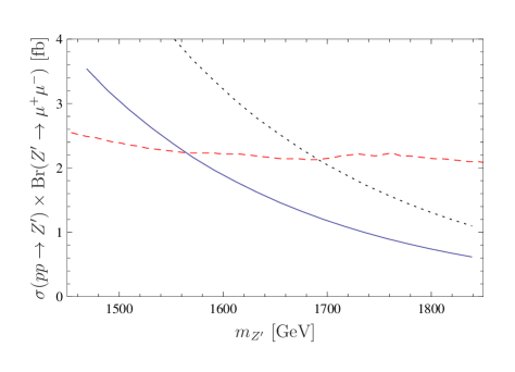
The appearance of additional final states leads to a reduction of the event numbers in the most sensitive search channels, i.e. reducing cross section times branching ratio, and, thus, the bounds obtained by the LHC collaborations ATLAS-CONF-2012-007 ; Collaboration:2011dca ; Chatrchyan:2011wq are less constraining in the BLR model. This is depicted in fig. 11 where we show the production cross section arround the resonance. 777For the calculation of the cross section we used WHIZARD Kilian:2007gr ; Moretti:2001zz and implemented the model using the SUSY Toolbox Staub:2011dp . In case that the width of the is calculated using only SM final states the cross section is increased roughly by a factor 1.6 in comparison to the case where also right handed neutrinos and SUSY particle contribute to the width of . With this choice of parameters, the main effect is due to R-neutrinos. We attribute the remaining difference to the official ATLAS result to slightly different values in the couplings and slightly different branching ratios of the final states. Our results agree also with the ones of ref. Erler:2011ud . We conclude that, although in our benchmark points we take always TeV, a significantly lower mass is possible consistent with data.
|
IV.4 Heavy neutrinos
As discussed above, the heavy neutrino states can be produced via the with a considerable branching ratio of about 30 per-cent when summing over all heavy neutrinos. Moreover, see below, they can also be produced in the cascade decays of supersymmetric particles. These heavy neutrinos mix with the light neutrino states implying a reduction of the couplings of the light neutrinos to the -boson and, thus, also a reduction of the invisible width of the -boson. Taking the data from ref. Nakamura:2010zzi this can be translated into the following condition on the sub-block , , of the neutrino mixing matrix:
| (79) |
at the 3- level. We have checked that all our benchmark points fullfill this condition.
The main decay modes of the heavy neutrinos are888 For related discussions see e.g. delAguila:2007em ; AguilarSaavedra:2009ik ; Das:2012ii and references therein.
| (80) | |||||
| (81) | |||||
| (82) |
where , , and , provided they are kinemtically allowed. If there is no kinematical suppression we find in general the branching ratios scale like where we have summed over the light Higgs bosons, the light neutrinos and leptons, respectively. We stress that these states are quasi-Dirac neutrinos and, thus, for six heavy neutrinos at LHC the existence of up to three new particles could be established. Note, that the final states containing a -boson allow for a direct mass measurement.
Beside the above decay modes, also decays into SUSY particle are possible if kinematics allow for it. For example we find that for BLRSP4 the decay into are possible and have branching ratios of about 3 per-cent. In scenarios like BLRSP3, BLRSP4 and BLRSP5 the main production of the heavy neutrinos is via the and, thus, a high luminosity will be required to observe such final states.
IV.5 SUSY cascade decays
In this section we point out several features which distinguish the BLR model from the usual MSSM. For the sake of preparing the ground, let us first summarize the main features of the MSSM relevant for the LHC, focusing for the time being on scenarios where the gluino is heavier than the squarks: (i) The gluino decays dominantly into squarks and quarks. (ii) L-squarks and L-sleptons decay dominantly into the chargino and the neutralino which are mainly -gauginos. Apart from kinematical effects the branching ratio for decays into the charged wino divided by the branching ratio into the neutral wino is about 2:1. (iii) R-squarks and R-sleptons decay dominantly into the bino-like neutralino with a branching ratio often quite close to 100 per-cent. (iv) In case of third generation sfermions also decays into higgsinos are important.
In the BLR model one has two main new features: (i) there are additional neutralinos and (ii) the sneutrino sector is enlarged as well. The latter implies that sneutrino LSPs are possible consistent with all astrophysical constraints and direct dark matter searches Gopalakrishna:2006kr ; Arina:2007tm ; Thomas:2007bu ; Cerdeno:2008ep ; Bandyopadhyay:2011qm ; Belanger:2011rs ; Dumont:2012ee . This feature is for example realised in study points BLRSP1 and BLRSP3999We note for completeness, that the relic abundance is actually somewhat too large in this point but can easily be adjusted by changing for example in BLRSP1 from 1.05 to 1.0475 without changing the collider features of BLRSP1..
Let us start the discussion with BLRSP1. In this point the four lighter neutralinos are the usual MSSM neutralinos with the standard hierarchy. The fifth state corresponds to the additional -gaugino, which we call , whereas the two additional states are the additional higgsinos. Note that the lighest neutralino is not stable anymore but decays into final states containing all nine neutrinos as well as the three lightest sneutrinos. Of the latter ones the second lightest is so long lived that it will lead to a displaced vertex in a typical collider detector. The third sneutrino decays dominatly via three-body decays into and with and . As discussed in section IV.4 the heavy neutrinos decay dominantly into -bosons and charged leptons, thus the decays of the lightest neutralino are not invisible.
appears for example in the decays of and with branching ratios BR( and BR(. For completeness we remark that the decays of and into is suppressed as the corresponding coupling is supressed as are the couplings of to -type quarks in this model. decays dominantly into sleptons and sneutrinos. Combining all the above together one gets a much richer structure for the decays of the R-squarks, e.g. the following decay chains:
| (83) | |||||
| (84) | |||||
| (85) | |||||
| (86) |
with and . Of course, several other combinations are possible as well.
From equations (83) to (86) one sees immediatly that the standard signature of R-squarks, namely jet and missing energy, is only realized in a few cases in this study point, e.g. if in eq. (83) the decays into neutrinos. Interestingly, the chain via into sleptons leads to a characteristic edge in the invariant mass of the lepton which can be used to determine the corresponding masses once combined with information from other decay chains. Also in the study points BLRSP2 and BLRSP5 and decay into heavy neutralinos, which contain sizable content of the extra gaugino, with a sizable branching ratio. However, there the situation is somewhat less involved as in these study points the lightest bino-like neutralino is the LSP.
Another interesting feature is, that decays also into the heavier sneutrinos which themselves decay into the LSP plus . Similarely can be produced in the decays of the heavy neutrinos implying that this state can be produced with sizable rate in SUSY cascade decays. However, as the corresponding final states are quite complicated a dedicated Monte Carlo study will be necessary to decide if this is indeed a discovery channel for .
From the point of view of SUSY cascade decays BLRSP2 looks essentially like a standard MSSM point. Inspection of the spectrum shows that is essentially a higgsino corresponding to the extended sector but it shows hardly up in the cascade decays. Its main production channel is via an -channel but even in this case the corresponding cross section is so low that it will not be dedected at the LHC even with an integrated luminosity of 300 fb-1. Another interesting feature shows up in the decays of which is mainly the neutral wino and gets copiously produced in the decays of the L-squarks: it decays with about 77 (15) per-cent into (), implying that the cascade decays are an important source of Higgs bosons.
In case of BLRSP3 one has sneutrino LSPs like in BLRSP1 but with a different hierarchy in the spectrum, as the three lightest sleptons are lighter then the lighest neutralino. Therefore the has also sizable decay rates into charged sleptons which sum to about 30 per-cent. The sleptons decay then further into and via 3-body decays into -pairs. The latter, however, are rather soft due to the small mass difference. In addition we have the decay channel into a light neutrino and one of the heavier sneutrinos which themselves decay into a lighter sneutrino and either one of the Higgs boson or the -boson. Putting again all these decays together one obtains for the decays
| (87) | |||||
| (88) | |||||
| (89) | |||||
| (90) | |||||
| (91) | |||||
| (92) |
with and . This implies that the decays of the R-squarks show again a more complicated structure compared to the usual CMSSM expectations. Channels (91) and (92) give in about 15 per-cent of the final states of . Moreover, and decay dominantly into sleptons and sneutrinos. Here a new feature is found for , as also the following chains
| (93) | |||||
| (94) |
gives rise to sharp edge structures. However, as the main final states of and are two jets, the feasability still needs to be investigated.
In BLRSP4 we have chosen GeV in order to construct an LSP which is essentially a . Here, the -sleptons are lighter than , which is essentially bino-like in this point, giving rise to the following decay chain of the down-type -squarks
| (95) |
Nearly all cascade decays end in a or one of the lighter sleptons. Due to the fact, that in this particular case the additional sneutrino states are hardly produced, it might be difficult to disthinguish it from the NMSSM, at least as long as the is not discovered. The heavier -sleptons do not show up in the cascade decays of squarks and gluinos but can be produced via the as discussed in section 4.
BLRSP5 is similar to BLRSP1 but compatible with pure GUT conditions, e.g. and are not input in this case put derived quantities. To fullfill the tadpole equations we have to choose and if we want a relatively low GeV while GeV. The choice of leads automatically to large masses for the heavy neutrinos such that the lightest Higgs can not decay into those states. As in BLRSP1 the down-type -squarks decay not only into but also into with a branching ratio of about 13 per-cent. For completeness, we note that here . However this state gets hardly produced in any of the SUSY decays or via the . Therefore, it is likely that LHC will miss it and also at a linear collider such as ILC or CLIC it will be difficult to study, due to the small production cross section.
V Conclusions
We have studied the minimal supersymmetric extension of the standard model. The model is minimal in the sense that the extended gauge symmetry is broken with the minimal number of Higgs fields. In the matter sector the model contains (three copies of) a superfield , to cancel anomalies. Adding three singlet superfields allows to generate small neutrino masses with an inverse seesaw mechanism.
The phenomenology of the model differs from the MSSM in a number of interesting aspects. We have foccused on the Higgs phenomenology and discussed changes in SUSY spectra and decays with respect to the MSSM. The model is less constrained then the CMSSM from the possible measurement of a Higgs with a mass of the order of 125 GeV. If the hints found in LHC data ATLAS:2012ae ; Chatrchyan:2012tx is indeed correct our model predicts two relatively light states should exist, with the second corresponding (mostly) to the lightest of the “right” Higgses, added to break the extended gauge group.
It is interesting, as we have discussed, that very often a right sneutrino is found to be the LSP. This will affect all constraints on CMSSM parameter space derived from constraints on the dark matter abundance. In fact, if the right sneutrino is indeed the LSP in our model, no constraint on any CMSSM parameters can be derived from DM constraints.
The model has new D-terms in all scalar mass matrices, which can lead to sizeable changes in the SUSY spectra, of potential phenomenological interest. We have discussed a few benchmark points, covering a number of features which could allow to distinguish the model from the CMSSM. Obviously this includes the discovery of a at the LHC where we have shown that the current bounds from LHC data depend on the details of the particle spectrum. Also the cascade decays of supersymmetric particles can be significantly more involved than in the usual CMSSM as the additional neutralinos, neutrinos and sneutrinos lead to enhancement of the multiplicities in the final states. This implies that the existing limits on the CMSSM parameter space get modified as standard final states have reduced branching ratios and at the same time additional final states are present. In case that the mBLR model is indeed realized these new cascade decays will offer additional kinematical information on the particle spectrum.
Acknowledgements
W.P. thanks the IFIC for hospitality during an extended stay. M.H. and L.R. acknowledge support from the Spanish MICINN grants FPA2011-22975, MULTIDARK CSD2009-00064 and by the Generalitat Valenciana grant Prometeo/2009/091 and the EU Network grant UNILHC PITN-GA-2009-237920. L.R thanks the Instituto Superior Técnico, Lisbon, for kind hospitality during an extended stay. W.P. has been supported by the Alexander von Humboldt foundation and in part by the DFG, project no. PO-1337/2-1 and the Helmholtz Alliance “Physics at the Terascale”.
Appendix A Appendix
A.1 Mass matrices
Here we list the tree-level mass matrices of the model not given in the main text.
-
•
Mass matrix for Down-Squarks, Basis:
(96) (97) (98) -
•
Mass matrix for Up-Squarks, Basis:
(99) (100) (101) -
•
Mass of the Charged Higgs boson: One obtains the same expression as in the MSSM:
(102) -
•
Mass matrix for Charginos, Basis:
(103)
A.2 Calculation of the mass spectrum
We are going to present now the basic steps to calculate the mass spectrum. As starting point we use electroweak precision data to get the gauge and Yukawa couplings: the SM-like Yukawa couplings are calculated from the fermion masses and the one-loop relations of ref. Pierce:1996zz which have been adjusted to our model. Similarly, also the standard model gauge couplings are calculated by the same procedure presented in ref. Pierce:1996zz , but again, including all new contributions of the mode under consideration. Since the entire RGE running is performed in the basis , the value of the GUT normalized and are matched to the GUT normalized hypercharge coupling by
| (104) | ||||
| (105) |
This is nothing else then an inversion of the well known relation between the gauge couplings for including the off-diagonal gauge couplings given in eq. (106). We are using the GUT normalization of for and for . To get the correct values of as well as and an iterative procedure is used: is calculated as ratio of the and when running down from the GUT scale and applying
| (106) |
When the gauge and Yukawa couplings are derived, the RGEs are then evaluated up to the GUT scale where the corresponding boundary conditions of eqs. (5), (6) and (12) are applied. Afterwards a RGE running of the full set of parameters to the SUSY scale is performed. We use always 2-loop RGEs which include the full effect of kinetic mixing Martin:1993zk ; Fonseca:2011vn .
The running parameters are then used to calculate the tree level mass spectrum. However, it is well known that the one-loop corrections can be very important for particular particles and have to be taken into account. The best known example is the light MSSM Higgs boson which get shifted by up to 50% per-cent in case of heavy stops. Similar effects can be expected in the extended Higgs sector especially since these can be very light at tree-level. Similarly, the gauginos arising in an extended gauge sector can be potentially light and receive important corrections at one-loop O'Leary:2011yq . To take these and all other possible effects into account we use a complete one-loop correction of the entire mass spectrum. Our procedure to calculate the one-loop masses is based on the method proposed in Ref.Pierce:1996zz : first, all running parameters are calculated at the SUSY scale and the SUSY masses at tree-level are derived. The EW vevs and are afterwards re-calculated using the one-loop corrected mass and demanding
| (107) |
in addition with the running value of . Note that as well as all other self-energies include the corrections originated by all particles present in the mBLR. These calculations are performed in scheme and ’t Hooft gauge. Also the complete dependence on the external momenta are taken into account. The re-calculated vevs are afterwards used to solve the tree-level tadpole equations again and to re-calculate the tree-level mass spectrum as well as all vertices entering the one-loop corrections. Using these vertices and masses, the one-loop corrections to the tadpole equations are derived and we use as renormalization condition
| (108) |
These one-loop corrected tadpole equations are solved with respect to the same parameter as at tree level resulting in new parameters , respectively , , . The final step is to calculate all self-energies for different particles and to use those to get the one-loop corrected mass spectrum.
-
1.
Real scalars: for a real scalar , the one-loop corrections are included by calculating the real part of the poles of the corresponding propagator matrices Pierce:1996zz
(109) where
(110) Equation (109) has to be solved for each eigenvalue which can be achieved in an iterative procedure. This has to be done also for charged scalars as well as the fermions. Note, is the tree-level mass matrix but for the parameters fixed by the tadpole equations the one-loop corrected values are used.
-
2.
Complex scalars: for a complex scalar field we use at one-loop level
(111) While in case of sfermions agrees exactly with the tree-level mass matrix, for charged Higgs bosons and or and has to be used depending on the set of parameters the tadpole equations are solved for.
-
3.
Majorana fermions: the one-loop mass matrix of a Majorana fermion is related to the tree-level mass matrix by
(112) where we have denoted the wave-function corrections by , and the direct one-loop contribution to the mass by .
-
4.
Dirac fermions: for a Dirac fermion one has to add the self-energies as
(113)
Note, this procedure agrees with the method implemented in SPheno 3.1.10 to calculate the loop masses in the MSSM as well as with the code produced by SARAH 3.0.39 or later. However, there are small differences to earlier versions of SPheno as well as other spectrum calculators: the MSSM equivalent of condition eq (107) is often solved in an iterative way using the one-loop corrected parameters from the tadpole equations to calculate until has converged. In this context also and are used in the vertices entering the one-loop corrections. However, these steps mix tree- and one-loop level and break therefore gauge invariance: when we tried this approach the relation between Goldstone and gauge bosons mass is violated. However, the numerical differences in case of the MSSM turned out to be rather small.
As example we give the necessary formulae to calculate the one-loop corrections to the tadpole equations and the scalar Higgs masses in appendix A.3.
A.3 1-loop corrections of the Higgs sector
As discussed in section A.2 we have calculated the entire mass spectrum at one-loop. For that purpose it is necessary to calculate all possible 1-loop diagrams for the one- and two-point functions. As example we here give the corresponding expressions for the one-loop corrections of the tadpoles as well as the self-energy for the scalar Higgs fields. For all other self-energies we refer to the output of SARAH 101010To get the model files of the mBLR which is not yet part of the public version of SARAH please send a mail to the authors.. The results are expressed via Passarino Veltman integrals Pierce:1996zz . The basic integrals are
| (114) | |||||
| (115) |
with the renormalization scale . All the other, necessary functions can be expressed by and . For instance,
| (116) |
and
| (117) | ||||
| (118) |
The numerical evalution of all loop-integrals is performed by SPheno. With this conventions we can write the one-loop tadpoles as
| (119) |
with . denotes the vertex of the three particles , , while will be used for four-point interactions. For chiral couplings we use as coefficient of the left and as coefficient of the right polarization operator. For instance, is the coupling of a pure down-type Higgs to a boson while corresponds to the left-chiral part of the interaction of a -Higgs to a neutralino of the second generation. The expressions for all vertices can be obtained with SARAH.
Using these conventions the self-energy for the scalar Higgs fields reads
| (120) |
A.4 RGEs
The calculation of the renormalization group equations performed by SARAH is
based on the generic
expression of Martin:1993zk . In addition, the results of
Fonseca:2011vn are used to
include the effect of kinetic mixing.
The functions for the parameters of a general superpotential written as
| (121) |
can be easily obtained from the shown results for the anomalous dimensions by using the relations West:1984dg ; Jones:1984cx
| (122) | |||||
| (123) |
For the results of the other parameters as well as for the two-loop results which we skip here because of their length we suggest to use the function CalcRGEs[] of SARAH.
A.4.1 Anomalous dimensions
| (124) | ||||
| (125) | ||||
| (126) | ||||
| (127) | ||||
| (128) | ||||
| (129) | ||||
| (130) | ||||
| (131) | ||||
| (132) | ||||
| (133) | ||||
| (134) |
A.4.2 Gauge Couplings
| (135) | ||||
| (136) | ||||
| (137) | ||||
| (138) | ||||
| (139) | ||||
| (140) |
A.4.3 Gaugino Mass Parameters
| (141) | ||||
| (142) | ||||
| (143) | ||||
| (144) | ||||
| (145) |
References
- (1) M. Malinsky, J. C. Romao and J. W. F. Valle, Phys. Rev. Lett. 95 (2005) 161801 [arXiv:hep-ph/0506296].
- (2) V. De Romeri, M. Hirsch, M. Malinsky, Phys. Rev. D84 053012 (2011); [arXiv:1107.3412 [hep-ph]].
- (3) R. Mohapatra and J. Valle, Phys. Rev. D34, 1642 (1986).
- (4) E. K. Akhmedov, M. Lindner, E. Schnapka and J. W. F. Valle, Phys. Rev. D 53, 2752 (1996) [hep-ph/9509255].
- (5) E. K. Akhmedov, M. Lindner, E. Schnapka and J. W. F. Valle, Phys. Lett. B 368, 270 (1996) [hep-ph/9507275].
- (6) M. Hirsch, M. Malinsky, W. Porod, L. Reichert and F. Staub, JHEP 1202, 084 (2012) [arXiv:1110.3037 [hep-ph]].
- (7) ATLAS Collaboration, G. Aad et al., Phys.Lett. B710, 49 (2012), arXiv:1202.1408.
- (8) CMS Collaboration, S. Chatrchyan et al., (2012), arXiv:1202.1488.
- (9) L. J. Hall, D. Pinner and J. T. Ruderman, arXiv:1112.2703 [hep-ph].
- (10) H. Baer, V. Barger and A. Mustafayev, arXiv:1112.3017 [hep-ph].
- (11) J. L. Feng, K. T. Matchev and D. Sanford, arXiv:1112.3021 [hep-ph].
- (12) S. Heinemeyer, O. Stal and G. Weiglein, arXiv:1112.3026 [hep-ph].
- (13) A. Arbey, M. Battaglia, A. Djouadi, F. Mahmoudi and J. Quevillon, Phys. Lett. B 708 (2012) 162 [arXiv:1112.3028 [hep-ph]].
- (14) A. Arbey, M. Battaglia and F. Mahmoudi, Eur. Phys. J. C 72 (2012) 1906 [arXiv:1112.3032 [hep-ph]].
- (15) P. Draper, P. Meade, M. Reece and D. Shih, arXiv:1112.3068 [hep-ph].
- (16) T. Moroi, R. Sato and T. T. Yanagida, Phys. Lett. B 709 (2012) 218 [arXiv:1112.3142 [hep-ph]].
- (17) M. Carena, S. Gori, N. R. Shah and C. E. M. Wagner, arXiv:1112.3336 [hep-ph].
- (18) U. Ellwanger, arXiv:1112.3548 [hep-ph].
- (19) O. Buchmueller, et al., arXiv:1112.3564 [hep-ph].
- (20) S. Akula, B. Altunkaynak, D. Feldman, P. Nath and G. Peim, arXiv:1112.3645 [hep-ph].
- (21) M. Kadastik, K. Kannike, A. Racioppi and M. Raidal, arXiv:1112.3647 [hep-ph].
- (22) J. Cao, Z. Heng, D. Li and J. M. Yang, arXiv:1112.4391 [hep-ph].
- (23) A. Arvanitaki and G. Villadoro, arXiv:1112.4835 [hep-ph].
- (24) M. Gozdz, arXiv:1201.0875 [hep-ph].
- (25) J. F. Gunion, Y. Jiang and S. Kraml, arXiv:1201.0982 [hep-ph].
- (26) G. G. Ross and K. Schmidt-Hoberg, arXiv:1108.1284 [hep-ph].
- (27) G. G. Ross, K. Schmidt-Hoberg and F. Staub, arXiv:1205.1509 [hep-ph].
- (28) P. Fileviez Perez, arXiv:1201.1501 [hep-ph].
- (29) N. Karagiannakis, G. Lazarides and C. Pallis, arXiv:1201.2111 [hep-ph].
- (30) S. F. King, M. Muhlleitner and R. Nevzorov, arXiv:1201.2671 [hep-ph].
- (31) Z. Kang, J. Li and T. Li, arXiv:1201.5305 [hep-ph].
- (32) C. -F. Chang, K. Cheung, Y. -C. Lin and T. -C. Yuan, arXiv:1202.0054 [hep-ph].
- (33) L. Aparicio, D. G. Cerdeno and L. E. Ibanez, arXiv:1202.0822 [hep-ph].
- (34) L. Roszkowski, E. M. Sessolo and Y. -L. S. Tsai, arXiv:1202.1503 [hep-ph].
- (35) J. Ellis and K. A. Olive, arXiv:1202.3262 [hep-ph].
- (36) H. Baer, V. Barger and A. Mustafayev, arXiv:1202.4038 [hep-ph].
- (37) N. Desai, B. Mukhopadhyaya and S. Niyogi, arXiv:1202.5190 [hep-ph].
- (38) J. Cao, Z. Heng, J. M. Yang, Y. Zhang and J. Zhu, arXiv:1202.5821 [hep-ph].
- (39) L. Maiani, A. D. Polosa and V. Riquer, arXiv:1202.5998 [hep-ph].
- (40) T. Cheng, J. Li, T. Li, D. V. Nanopoulos and C. Tong, arXiv:1202.6088 [hep-ph].
- (41) N. Christensen, T. Han and S. Su, arXiv:1203.3207 [hep-ph].
- (42) D. A. Vasquez, G. Belanger, C. Boehm, J. Da Silva, P. Richardson and C. Wymant, arXiv:1203.3446 [hep-ph].
- (43) U. Ellwanger and C. Hugonie, arXiv:1203.5048 [hep-ph].
- (44) Updated results can be found on the web-page: https://twiki.cern.ch/twiki/bin/view/AtlasPublic; see, especially: ATLAS-CONF-2012-033
-
(45)
Updated results can be found on the web-page:
https://twiki.cern.ch/twiki/bin/view/CMSPublic/PhysicsResults - (46) H. E. Haber, M. Sher, Phys. Rev. D35 (1987) 2206.
- (47) M. Drees, Phys. Rev. D35 (1987) 2910-2913.
- (48) M. Cvetic, D. A. Demir, J. R. Espinosa, L. L. Everett, P. Langacker, Phys. Rev. D56 (1997) 2861. [hep-ph/9703317].
- (49) Y. Zhang, H. An, X. d. Ji and R. N. Mohapatra, Phys. Rev. D 78, 011302 (2008) [arXiv:0804.0268 [hep-ph]].
- (50) E. Ma, [arXiv:1108.4029 [hep-ph]].
- (51) K. Nakamura et al. [Particle Data Group Collaboration], J. Phys. G G 37, 075021 (2010).
- (52) T. Falk, K. A. Olive and M. Srednicki, Phys. Lett. B 339, 248 (1994) [hep-ph/9409270].
- (53) A. Ali, D. A. Demir, M. Frank and I. Turan, Phys. Rev. D 79 (2009) 095001 [arXiv:0902.3826 [hep-ph]].
- (54) A. Belyaev, J. P. Hall, S. F. King and P. Svantesson, arXiv:1203.2495 [hep-ph].
- (55) S. P. Martin, Phys. Rev. D 46, 2769 (1992) [hep-ph/9207218].
- (56) B. C. Allanach et al., Comput. Phys. Commun. 180 (2009) 8-25. [arXiv:0801.0045 [hep-ph]].
- (57) B. Holdom, Phys. Lett. B 166, 196 (1986).
- (58) K. S. Babu, C. F. Kolda and J. March-Russell, Phys. Rev. D 57 (1998) 6788 [arXiv:hep-ph/9710441].
- (59) R. Fonseca, M. Malinsky, W. Porod, F. Staub, Nucl. Phys. B854 (2012) 28-53. [arXiv:1107.2670 [hep-ph]].
- (60) B. O’Leary, W. Porod and F. Staub, JHEP 1205 (2012) 042 [arXiv:1112.4600 [hep-ph]].
- (61) F. Braam and J. Reuter, arXiv:1107.2806 [hep-ph].
- (62) E. J. Chun, J. -C. Park and S. Scopel, JHEP 1102 (2011) 100 [arXiv:1011.3300 [hep-ph]].
- (63) Y. Mambrini, JCAP 1107, 009 (2011) [arXiv:1104.4799 [hep-ph]].
- (64) T. G. Rizzo, Phys. Rev. D 85, 055010 (2012) [arXiv:1201.2898 [hep-ph]].
- (65) D. Matalliotakis and H. P. Nilles, Nucl. Phys. B 435, 115 (1995) [hep-ph/9407251].
- (66) N. Polonsky and A. Pomarol, Phys. Rev. D 51, 6532 (1995) [hep-ph/9410231].
- (67) V. Berezinsky, A. Bottino, J. R. Ellis, N. Fornengo, G. Mignola and S. Scopel, Astropart. Phys. 5, 1 (1996) [hep-ph/9508249].
- (68) D. M. Pierce, J. A. Bagger, K. T. Matchev, R. -j. Zhang, Nucl. Phys. B491 (1997) 3-67. [hep-ph/9606211].
- (69) W. Porod, Comput. Phys. Commun. 153 (2003) 275 [arXiv:hep-ph/0301101].
- (70) W. Porod and F. Staub, arXiv:1104.1573 [hep-ph].
- (71) F. Staub, arXiv:0806.0538 [hep-ph].
- (72) F. Staub, arXiv:0909.2863 [hep-ph].
- (73) F. Staub, Comput. Phys. Commun. 182 (2011) 808 [arXiv:1002.0840 [hep-ph]].
- (74) ATLAS conference note ATLAS-CONF-2012-007, see ATLAS-WEB
- (75) J. Erler, P. Langacker, S. Munir, E. Rojas, [arXiv:1103.2659 [hep-ph]].
- (76) M. Hirsch, H. V. Klapdor-Kleingrothaus and S. G. Kovalenko, Phys. Lett. B 398, 311 (1997) [hep-ph/9701253].
- (77) M. Hirsch, J. W. F. Valle, W. Porod, J. C. Romao and A. Villanova del Moral, Phys. Rev. D 78 (2008) 013006 [arXiv:0804.4072 [hep-ph]].
- (78) M. Hirsch, S. Kaneko and W. Porod, Phys. Rev. D 78, 093004 (2008) [arXiv:0806.3361 [hep-ph]].
- (79) J. N. Esteves, J. C. Romao, M. Hirsch, F. Staub and W. Porod, Phys. Rev. D 83, 013003 (2011) [arXiv:1010.6000 [hep-ph]].
- (80) M. Hirsch, F. Staub and A. Vicente, arXiv:1202.1825 [hep-ph].
- (81) J. Adam et al. [MEG collaboration], Phys. Rev. Lett. 107 (2011) 171801 [arXiv:1107.5547 [hep-ex]].
- (82) P. Bechtle, O. Brein, S. Heinemeyer, G. Weiglein and K. E. Williams, Comput. Phys. Commun. 181 (2010) 138 [arXiv:0811.4169 [hep-ph]].
- (83) P. Bechtle, O. Brein, S. Heinemeyer, G. Weiglein and K. E. Williams, arXiv:1102.1898 [hep-ph].
- (84) G. Degrassi, P. Slavich and F. Zwirner, Nucl. Phys. B 611 (2001) 403.
- (85) A. Brignole, G. Degrassi, P. Slavich and F. Zwirner, Nucl. Phys. B 631 (2002) 195.
- (86) A. Brignole, G. Degrassi, P. Slavich and F. Zwirner, Nucl. Phys. B 643 (2002) 79.
- (87) A. Dedes and P. Slavich, Nucl. Phys. B 657 (2003) 333.
- (88) A. Dedes, G. Degrassi and P. Slavich, Nucl. Phys. B 672 (2003) 144.
- (89) B. C. Allanach, A. Djouadi, J. L. Kneur, W. Porod and P. Slavich, JHEP 0409 (2004) 044 [hep-ph/0406166].
- (90) A. Nisati, for the ATLAS collaboration, talk presented at Lepton-Photon Conference 2011, Mumbai, India, August 2011.
- (91) V. Sharma, for the CMS collaboration, talk presented at Lepton-Photon Conference 2011, Mumbai, India, August 2011.
- (92) E. Etzion, private communication.
- (93) G. Aad et al. [ATLAS Collaboration], Phys. Rev. Lett. 107 (2011) 272002 [arXiv:1108.1582 [hep-ex]].
- (94) S. Chatrchyan et al. [CMS Collaboration], JHEP 1105 (2011) 093 [arXiv:1103.0981 [hep-ex]].
- (95) W. Kilian, T. Ohl and J. Reuter, Eur. Phys. J. C 71, 1742 (2011) [arXiv:0708.4233 [hep-ph]].
- (96) M. Moretti, T. Ohl and J. Reuter, arXiv:hep-ph/0102195.
- (97) F. Staub, T. Ohl, W. Porod, C. Speckner, [arXiv:1109.5147 [hep-ph]].
- (98) B. Fuks, M. Klasen, F. Ledroit, Q. Li and J. Morel, Nucl. Phys. B 797 (2008) 322 [arXiv:0711.0749 [hep-ph]].
- (99) F. del Aguila, J. A. Aguilar-Saavedra and R. Pittau, JHEP 0710 (2007) 047 [hep-ph/0703261].
- (100) J. A. Aguilar-Saavedra, Nucl. Phys. B 828 (2010) 289 [arXiv:0905.2221 [hep-ph]].
- (101) S. P. Das, F. F. Deppisch, O. Kittel and J. W. F. Valle, arXiv:1206.0256 [hep-ph].
- (102) S. Gopalakrishna, A. de Gouvea and W. Porod, JCAP 0605 (2006) 005 [hep-ph/0602027].
- (103) C. Arina and N. Fornengo, JHEP 0711 (2007) 029 [arXiv:0709.4477 [hep-ph]].
- (104) Z. Thomas, D. Tucker-Smith and N. Weiner, Phys. Rev. D 77 (2008) 115015 [arXiv:0712.4146 [hep-ph]].
- (105) D. G. Cerdeno, C. Munoz and O. Seto, Phys. Rev. D 79 (2009) 023510 [arXiv:0807.3029 [hep-ph]].
- (106) P. Bandyopadhyay, E. J. Chun and J. -C. Park, JHEP 1106 (2011) 129 [arXiv:1105.1652 [hep-ph]].
- (107) G. Belanger, J. Da Silva and A. Pukhov, JCAP 1112 (2011) 014 [arXiv:1110.2414 [hep-ph]].
- (108) B. Dumont, G. Belanger, S. Fichet, S. Kraml and T. Schwetz, arXiv:1206.1521 [hep-ph].
- (109) S. P. Martin and M. T. Vaughn, Phys. Rev. D 50 (1994) 2282 [Erratum-ibid. D 78 (2008) 039903] [arXiv:hep-ph/9311340].
- (110) P. C. West, Phys. Lett. B 137 (1984) 371.
- (111) D. R. T. Jones and L. Mezincescu, Phys. Lett. B 138, 293 (1984).