Monochromatic triangles in three-coloured graphs

Abstract.

In 1959, Goodman [8] determined the minimum number of monochromatic triangles in a complete graph whose edge set is $2$-coloured. Goodman [9] also raised the question of proving analogous results for complete graphs whose edge sets are coloured with more than two colours. In this paper, for $n$ sufficiently large, we determine the minimum number of monochromatic triangles in a $3$-coloured copy of $K_{n}$. Moreover, we characterise those $3$-coloured copies of $K_{n}$ that contain the minimum number of monochromatic triangles.

1. Introduction

The Ramsey number $R_{k}(G)$ of a graph $G$ is the minimum $n\in\mathbb{N}$ such that every $k$-colouring of $K_{n}$ contains a monochromatic copy of $G$. (In this paper we say a graph $K$ is $k$-coloured if we have coloured the edge set of $K$ using $k$ colours. Note that the edge colouring need not be proper.) A famous theorem of Ramsey [16] asserts that $R_{k}(G)$ exists for all graphs $G$ and all $k\in\mathbb{N}$.

In light of this, it is also natural to consider the so-called Ramsey multiplicity of a graph: Let $k,n\in\mathbb{N}$ and let $G$ be a graph. The Ramsey multiplicity $M_{k}(G,n)$ of $G$ is the minimum number of monochromatic copies of $G$ over all $k$-colourings of $K_{n}$. (Here, we are counting unlabelled copies of $G$ in the sense that we count the number of distinct monochromatic subgraphs of $K_{n}$ that are isomorphic to $G$.) In the case when $k=2$ we simply write $M(G,n)$. The following classical result of Goodman [8] from 1959 gives the precise value of $M(K_{3},n)$.

Theorem 1 (Goodman [8]).

Let $n\in\mathbb{N}$. Then

$$M(K_{3},n)=\left\{\begin{array}[]{ll}n(n-2)(n-4)/24&\text{if $n$ is even;}\\ n(n-1)(n-5)/24&\text{if $n\equiv 1\mod 4$;}\\ (n+1)(n-3)(n-4)/24&\text{if $n\equiv 3\mod 4.$}\end{array}\right.$$

A graph $G$ is $k$-common if $M_{k}(G,n)$ asymptotically equals, as $n$ tends to infinity, the expected number of monochromatic copies of $G$ in a random $k$-colouring of $K_{n}$. Erdős [5] conjectured that $K_{r}$ is $2$-common for every $r\in\mathbb{N}$. Note that Theorem 1 implies that this conjecture is true for $r=3$. However, Thomason [21, 22] disproved the conjecture in the case when $r=4$. Further, Jagger, Šťovíček, and Thomason [12] proved that any graph $G$ that contains $K_{4}$ is not $2$-common. Recently, Cummings and Young [4] proved that graphs $G$ that contain $K_{3}$ are not $3$-common. The introductions of [4] and [11] give more detailed overviews of $k$-common graphs.

The best known general lower bound on $M(K_{r},n)$ was proved by Conlon [3]. Some general bounds on $M_{k}(K_{r},n)$ are given in [6]. See [2] for a (somewhat outdated) survey on Ramsey multiplicities.

The problem of obtaining a $3$-coloured analogue of Goodman’s theorem also has a long history. In fact, it is not entirely clear when this problem was first raised. In 1985, Goodman [9] simply refers to it as “an old and difficult problem”. Prior to this, Giraud [7] proved that, for sufficiently large $n$, $M_{3}(K_{3},n)>4\binom{n}{3}/115$. Wallis [23] showed that $M_{3}(K_{3},17)\leq 5$ and then, together with Sane [19], proved that $M_{3}(K_{3},17)=5$. (Greenwood and Gleason [10] proved that $R_{3}(K_{3})=17$, therefore, $M_{3}(K_{3},16)=0$.)

The focus of this paper is to give the exact value of $M_{3}(K_{3},n)$ for sufficiently large $n$, thereby yielding a $3$-coloured analogue of Goodman’s theorem. Moreover, we characterise those $3$-coloured copies of $K_{n}$ that contain exactly $M_{3}(K_{3},n)$ monochromatic triangles.

Given $n\in\mathbb{N}$ we define a special collection of $3$-coloured complete graphs on $n$ vertices, $\mathcal{G}_{n}$ as follows:

• Consider the (unique) $2$-coloured copy $K$ of $K_{5}$ on $[5]$ without a monochromatic triangle. Replace the vertices of $K$ with disjoint vertex classes $V_{1},\dots,V_{5}$ such that $||V_{i}|-|V_{j}||\leq 1$ for all $1\leq i,j\leq 5$ and $|V_{1}|+\dots+|V_{5}|=n$. For all $1\leq i\not=j\leq 5$, add all possible edges between $V_{i}$ and $V_{j}$ using the colour of $ij$ in $K$. For each $1\leq i\leq 5$, add all possible edges inside $V_{i}$ in a third colour. Denote the resulting complete $3$-coloured graph by $G_{ex}(n)$ (see Figure 1).

• $\mathcal{G}_{n}$ consists of $G_{ex}(n)$ together with all graphs obtained from $G_{ex}(n)$ by recolouring a (possibly empty) matching $M_{i,j}$ in $G_{ex}(n)[V_{i},V_{j}]$ with the third colour for all $1\leq i\not=j\leq 5$, such that the recolouring does not introduce any new monochromatic triangles (see Figure 1).

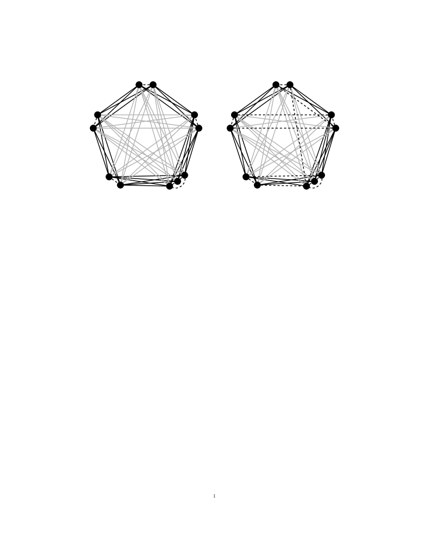
Figure 1. $G_{ex}(11)$ and another element of $\mathcal{G}_{11}$

Notice that the graphs in $\mathcal{G}_{n}$ only contain monochromatic triangles of one colour. The following is our main result.

Theorem 2.

There exists an $n_{0}\in\mathbb{N}$ such that the following holds. Suppose $G$ is a complete $3$-coloured graph on $n\geq n_{0}$ vertices which contains the smallest number of monochromatic triangles amongst all complete $3$-coloured graphs on $n$ vertices. Then $G$ is a graph from $\mathcal{G}_{n}$.

Corollary 3.

There exists an $n_{0}\in\mathbb{N}$ such that the following holds. Suppose $n\geq n_{0}$ and write $n=5m+r$ where $m,r\in\mathbb{N}$ such that $0\leq r\leq 4$. Then

$$M_{3}(K_{3},n)=r\binom{m+1}{3}+(5-r)\binom{m}{3}.$$

The proof of Theorem 2 uses Razborov’s method of flag algebras [17] together with a probabilistic argument.

Goodman [9] also raised the question of establishing $k$-coloured analogues of Theorem 1 for $k\geq 4$. Let $k\geq 3$ and $n\in\mathbb{N}$. Fox [6] gave an upper bound on $M_{k}(K_{3},n)$ by considering the following graphs: Set $m:=R_{k-1}(K_{3})-1$. Consider a $(k-1)$-coloured copy $K$ of $K_{m}$ on $[m]$ without a monochromatic triangle. Replace the vertices of $K$ with disjoint vertex classes $V_{1},\dots,V_{m}$ such that $||V_{i}|-|V_{j}||\leq 1$ for all $1\leq i,j\leq m$ and $|V_{1}|+\dots+|V_{m}|=n$. For all $1\leq i\not=j\leq m$, add all possible edges between $V_{i}$ and $V_{j}$ using the colour of $ij$ in $K$. For each $1\leq i\leq m$, add all possible edges to $V_{i}$ using a $k$th colour. Denote the resulting complete $k$-coloured graph by $G_{ex}(n,k)$. (Thus, $G_{ex}(n)=G_{ex}(n,3)$.)

Question 4.

Let $k\geq 4$ and $n\in\mathbb{N}$ be sufficiently large. Is $M_{k}(K_{3},n)$ equal to the number of monochromatic triangles in $G_{ex}(n,k)$?

2. Notation

We will make the convention that the set of colours used in a $k$-colouring of the edges of a graph is $[k]$. In the case of a $3$-colouring we will generally refer to the colours $1$, $2$ and $3$ as “red”, “blue” and “green”. When $H$ and $H^{\prime}$ are two $k$-coloured graphs, an isomorphism between them is a function $f:V(H)\rightarrow V(H^{\prime})$ which is a graph isomorphism and respects the colouring. Two $k$-coloured graphs $H$ and $H^{\prime}$ are isomorphic ($H\cong H^{\prime}$) if and only if there is an isomorphism between them.

Given $r\in\mathbb{N}$, we denote the complete graph on $r$ vertices by $K_{r}$ and define $R(r,r):=R_{2}(K_{r})$. Given $k$ and $c\in[k]$, we define $K^{r}_{c}$ to be the $k$-coloured complete graph in which every edge of $K_{r}$ is given the colour $c$. We define ${\mathcal{K}}^{r}$ to be $\{K^{r}_{c}:c\in[k]\}$, that is to say the set of monochromatic $K_{r}$’s. Suppose $G$ is a $k$-coloured graph and let $v\in V(G)$ and $i\in[k]$. Then we will use $N_{i}(v)$ to denote the set of vertices in $G$ that receive an edge of colour $i$ from $v$.

For a graph $G$ and a vertex set $V\subseteq V(G)$, we denote by $G[V]$ the subgraph of $G$ induced by $V$. Given $v_{1},\dots,v_{m}\in V(G)$ we write $G[v_{1},\dots,v_{m}]$ for $G[\{v_{1},\dots,v_{m}\}]$, and for disjoint subsets $V$ and $W$ of $V(G)$ we denote by $G[V,W]$ the bipartite graph with vertex classes $V$ and $W$ whose edge set consists of those edges between $V$ and $W$ in $G$. When $G$ is a $k$-coloured graph, we view $G[V]$ as a $k$-coloured graph with the edge colouring inherited from $G$, and do likewise for $G[v_{1},\dots,v_{m}]$ and for $G[V,W]$.

Throughout the paper, we write, for example, $0<\nu\ll\tau\ll\eta$ to mean that we can choose the constants $\nu,\tau,\eta$ from right to left. More precisely, there are increasing functions $f$ and $g$ such that, given $\eta$, whenever we choose some $\tau\leq f(\eta)$ and $\nu\leq g(\tau)$, all calculations needed in our proof are valid. Hierarchies with more constants are defined in the obvious way. Finally, the set of all $k$-subsets of a set $A$ is denoted by $[A]^{k}$.

In the proof of Theorem 2 we will omit floors and ceilings whenever this does not affect the argument.

3. Graph densities

From this point on we are exclusively concerned with $3$-colourings, mostly colourings of complete graphs. Suppose $H$ and $G$ are $3$-coloured complete graphs where $|H|\leq|G|$. Let $d(H,G)$ denote the number of sets $V\in[V(G)]^{|H|}$ such that $G[V]\cong H$, and define the density of $H$ in $G$ as

$$p(H,G):=\frac{d(H,G)}{\binom{|G|}{|H|}}.$$

This quantity has a natural probabilistic interpretation, namely it is the probability that if we choose a set ${\mathbf{V}}\in[V(G)]^{|H|}$ uniformly at random then ${\mathbf{V}}$ induces an isomorphic copy of $H$.

When $\mathcal{H}$ is a family of $3$-coloured complete graphs $H$ of some fixed size $k$ with $k\leq|G|$, we define

$$p(\mathcal{H},G):=\sum_{H\in{\mathcal{H}}}p(H,G),$$

that is to say the probability that a random ${\mathbf{V}}\in[V(G)]^{k}$ induces a coloured graph isomorphic to an element of $\mathcal{H}$. In the sequel we generally write “$H^{\prime}$ is an $\mathcal{H}$” as an abbreviation for “$H^{\prime}$ is isomorphic to some $H\in{\mathcal{H}}$”, “$G$ contains an $\mathcal{H}$” as an abbreviation for “$G$ contains an induced isomorphic copy of an element of $\mathcal{H}$”, and “an $\mathcal{H}$ in $G$” for “an induced copy of some element of $\mathcal{H}$ in $G$”.

For $n\geq|H|$ we let $p^{\rm min}(H,n)$ be the minimum value of $p(H,G)$ over all $3$-coloured complete graphs $G$ on $n$ vertices. When $\mathcal{H}$ is a family of $3$-coloured complete graphs $H$ of some fixed size $k\leq n$, we let $p^{\rm min}({\mathcal{H}},n)$ be the minimum value of $p({\mathcal{H}},G)$ over all $3$-coloured complete graphs $G$ on $n$ vertices.

We now define a certain class $\mathcal{H}$ of “bad” $3$-coloured complete graphs on $4$ vertices. As motivation, we note that we are defining a set of $3$-coloured graphs $H$ such that $\max_{G\in{\mathcal{G}}_{n}}p(H,G)\rightarrow 0$ with increasing $n$.

Let ${\mathcal{H}}(i,j,k)$ be the class of $3$-coloured complete graphs on $4$ vertices with a monochromatic triangle, $i$ extra edges of that same colour, and $j$ and $k$ edges of the other colours, respectively (with $i+j+k=3$, $j\geq k$). Define $\mathcal{H}:={\mathcal{H}}(2,1,0)\cup{\mathcal{H}}(1,1,1)\cup{\mathcal{H}}(0,2,1)$.

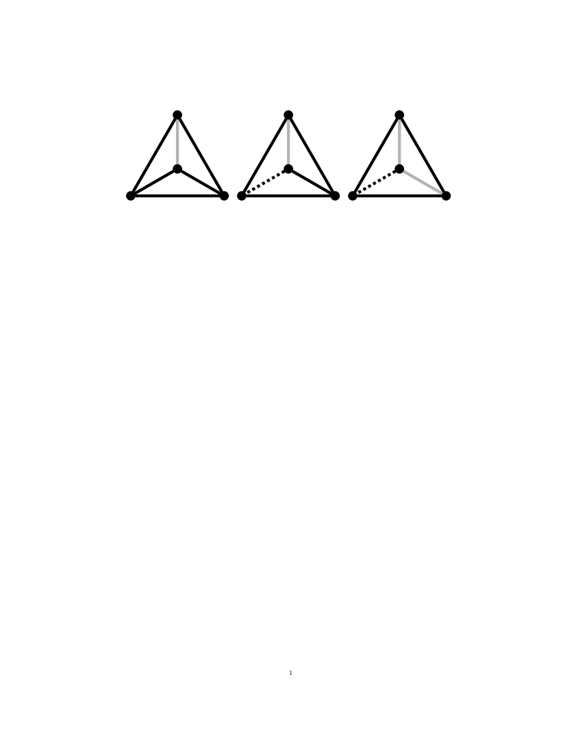
Figure 2. Representative elements of ${\mathcal{H}}(2,1,0)$, ${\mathcal{H}}(1,1,1)$ and ${\mathcal{H}}(0,2,1)$.

The following result about graph densities will be used in the proof of Theorem 2. It provides an (asymptotically) optimal lower bound on the density of monochromatic triangles, and also asserts that copies of colourings from the class $\mathcal{H}$ are rare in any colouring that comes close enough to achieving this bound. The proof is given in Section 4.

Proposition 5.

For all $\varepsilon>0$ there is $n_{0}$ such that for all $3$-coloured complete graphs $G$ on at least $n_{0}$ vertices:

1. $p({\mathcal{K}}^{3},G)\geq 0.04-\varepsilon$.

2. If $p({\mathcal{K}}^{3},G)\leq 0.04$, then $p({\mathcal{H}},G)<\varepsilon$.

4. Flag algebras

In this section we use the method of flag algebras due to Razborov [17] to prove Proposition 5. The flag machinery described in subsections 4.1 and 4.2 is due to Razborov, as is the idea of using semidefinite programming for search of valid inequalities using this framework.

4.1. Some background

We start by describing how the main concepts of the general theory of flag algebras look in the case of $3$-coloured complete graphs. Let ${\mathcal{M}}_{l}$ be the set of isomorphism classes of $3$-coloured complete graphs on $l$ vertices. It is helpful to know $|{\mathcal{M}}_{l}|$ for small values of $l$; computing this value is a classical enumeration problem [20], in particular $|{\mathcal{M}}_{l}|=1,1,3,10,66,792$ for $l=0,1,2,3,4,5$.

A type $\sigma$ is a $3$-coloured complete graph whose underlying set is of the form $[k]=\{1,2,\ldots,k\}$ for some $k$, where we write $|\sigma|=k$. A $\sigma$-flag is a $3$-coloured complete graph which contains a labelled copy of $\sigma$, or more formally a pair $(M,\theta)$ where $M$ is a $3$-coloured complete graph and $\theta$ is an injective map from $[k]$ to $V(M)$ that respects the edge-colouring of $\sigma$. Two $\sigma$-flags are isomorphic if there is an isomorphism that respects the labelling. More formally, $f$ is a flag isomorphism from $(M_{1},\theta_{1})$ to $(M_{2},\theta_{2})$ if $f:V(M_{1})\rightarrow V(M_{2})$ is an isomorphism of coloured graphs and $\sigma\circ\theta_{1}=\theta_{2}$.

We denote by ${\mathcal{F}}^{\sigma}_{l}$ the set of isomorphism classes of $\sigma$-flags with $l$ vertices. Note that if $0$ is the empty type then ${\mathcal{F}}^{0}_{l}={\mathcal{M}}_{l}$. The flags of most interest to us are the elements of ${\mathcal{F}}^{\sigma}_{4}$ for various $\sigma$ with $|\sigma|=3$; it is easy to see that if $|\sigma|=3$ then $|{\mathcal{F}}^{\sigma}_{4}|=27$.

The notion of graph density described in the preceding section extends to $\sigma$-flags in a straightforward way. Given $\sigma$-flags $F\in{\mathcal{F}}^{\sigma}_{l}$ and $G\in{\mathcal{F}}^{\sigma}_{m}$ for $m\geq l$, we define $p(F,G)$ to be the density of isomorphic copies of $F$ in $G$. More formally let $G=(M,\theta)$, choose uniformly at random a set ${\mathbf{V}}\in[V(M)]^{l}$ such that ${\mathbf{V}}$ contains $\operatorname{im}(\theta)$, and define $p(F,G)$ to be the probability that $(M[{\mathbf{V}}],\theta)$ is isomorphic (as a $\sigma$-flag) to $F$. By convention we will set $p(F,G)=0$ in case $m<l$.

It is routine to see that if $l\leq m\leq n$, $F\in{\mathcal{F}}^{\sigma}_{l}$ and $H\in{\mathcal{F}}^{\sigma}_{n}$ then

(1) $$p(F,H)=\sum_{G\in{\mathcal{F}}^{\sigma}_{m}}p(F,G)p(G,H).$$

This chain rule plays a central role in the theory.

More generally, given flags $F_{i}\in{\mathcal{F}}^{\sigma}_{l_{i}}$ for $1\leq i\leq n$ and $G=(M,\theta)\in{\mathcal{F}}^{\sigma}_{m}$ where $m\geq\sum_{i}l_{i}-(n-1)|\sigma|$, we define a “joint density” $p(F_{1},\ldots,F_{n};G)$. This is the probability that if we choose an $n$-tuple $({\mathbf{V}}_{1},\ldots,{\mathbf{V}}_{n})$ of subsets of $V(M)$ uniformly at random, subject to the conditions ${\mathbf{V}}_{i}\in[V(M)]^{l_{i}}$ and ${\mathbf{V}}_{i}\cap{\mathbf{V}}_{j}=\operatorname{im}(\theta)$ for $i\neq j$, then $(M[{\mathbf{V}}_{i}],\theta)$ is isomorphic to $F_{i}$ for all $i$.

A sequence $(G_{n})$ of $\sigma$-flags is said to be increasing if the number of vertices in $G_{n}$ tends to infinity, and convergent if the sequence of densities $(p(F,G_{n}))$ converges for every $\sigma$-flag $F$. A routine argument along the lines of the Bolzano-Weierstrass theorem shows that every increasing sequence has a convergent subsequence. If $(G_{n})$ is convergent then we can define a map $\Phi$ on $\sigma$-flags by setting $\Phi(F)=\lim_{n\rightarrow\infty}p(F,G_{n})$. We note that when $F\in{\mathcal{F}}^{\sigma}_{l}$ and $l\leq m$, it follows readily from equation (1) that

(2) $$\Phi(F)=\sum_{G\in{\mathcal{F}}^{\sigma}_{m}}p(F,G)\Phi(G).$$

Equation (2) suggests that in some sense “$F=\sum_{G\in{\mathcal{F}}^{\sigma}_{m}}p(F,G)G$”, and the definition of the flag algebra ${\mathcal{A}}^{\sigma}$ makes this precise. We define ${\mathcal{F}}^{\sigma}_{\infty}=\bigcup_{n}{\mathcal{F}}^{\sigma}_{n}$, let ${\mathbb{R}}{\mathcal{F}}^{\sigma}_{\infty}$ be the real vector space consisting of finite formal linear combinations of elements of ${\mathcal{F}}^{\sigma}_{\infty}$, and then define ${\mathcal{A}}^{\sigma}$ to be the quotient of ${\mathbb{R}}{\mathcal{F}}^{\sigma}_{\infty}$ by the subspace ${\mathcal{K}}^{\sigma}$ generated by all elements of the form $F-\sum_{G\in{\mathcal{F}}^{\sigma}_{m}}p(F,G)G$. We will not be distinguishing between a flag $F$, its isomorphism class $[F]\in{\mathcal{F}}^{\sigma}$, the element $1[F]\in{\mathbb{R}}{\mathcal{F}}^{\sigma}_{\infty}$ and the element $1[F]+{\mathcal{K}}^{\sigma}\in{\mathcal{A}}^{\sigma}$.

If $\Phi$ is the map on $\sigma$-flags induced by a convergent sequence as above, then $\Phi$ extends by linearity to a map $\Phi:{\mathbb{R}}{\mathcal{F}}^{\sigma}_{\infty}\rightarrow{\mathbb{R}}$. The linear map $\Phi$ vanishes on ${\mathcal{K}}^{\sigma}$ by equation (2), and hence induces a linear map $\Phi:{\mathcal{A}}^{\sigma}\rightarrow{\mathbb{R}}$. So far ${\mathcal{A}}^{\sigma}$ is only a real vector space; we make it into an $\mathbb{R}$-algebra by defining a product as follows. Let $F_{1}\in{\mathcal{F}}^{\sigma}_{l_{1}}$, $F_{2}\in{\mathcal{F}}^{\sigma}_{l_{2}}$, let $m\geq l_{1}+l_{2}-|\sigma|$, and define

$$F_{1}\cdot F_{2}:=\sum_{G\in{\mathcal{F}}^{\sigma}_{m}}p(F_{1},F_{2};G)G.$$

This can be shown [17, Lemma 2.4] to give a well-defined multiplication operation on ${\mathcal{A}}^{\sigma}$ independent of the choice of $m$, and it can also be shown [17, Theorem 3.3 part a] that if $\Phi:{\mathcal{A}}^{\sigma}\rightarrow{\mathbb{R}}$ is induced by a convergent sequence then $\Phi(F_{1}\cdot F_{2})=\Phi(F_{1})\Phi(F_{2})$, that is $\Phi$ is an algebra homomorphism from ${\mathcal{A}}^{\sigma}$ to ${\mathbb{R}}$. The converse is also true [17, Theorem 3.3 part b]: if $\Phi$ is such a homomorphism and $\Phi(F)\geq 0$ for all $\sigma$-flags $F$, then there exists an increasing and convergent sequence $(G_{n})$ such that $\Phi(F)=\lim_{n}p(F,G_{n})$ for all flags $F$.

Following Razborov we let $\mathrm{Hom}^{+}({\mathcal{A}}^{\sigma},{\mathbb{R}})$ be the set of homomorphisms induced by convergent sequences of $\sigma$-flags, and define a preordering on ${\mathcal{A}}^{\sigma}$ by stipulating that $A\leq B$ if and only if $\Phi(A)\leq\Phi(B)$ for all $\Phi\in\mathrm{Hom}^{+}({\mathcal{A}}^{\sigma},{\mathbb{R}})$.

4.2. Averaging and lower bounds

The algebra ${\mathcal{A}}^{\sigma}$ has an identity element $1_{\sigma}=(\sigma,id_{\sigma})$, and it is easy to see that $\Phi(1^{\sigma})=1$ for all $\Phi\in\mathrm{Hom}^{+}({\mathcal{A}}^{\sigma},{\mathbb{R}})$. Accordingly we will identify the real number $r$ and the element $r1_{\sigma}$. With this convention, the task of finding asymptotic lower bounds for quantities like the density of monochromatic triangles amounts to proving inequalities of the form “$F\geq r$ in ${\mathcal{A}}^{0}$” for some sum of $0$-flags $F$ and real number $r$. We will prove that

$$K^{3}_{red}+K^{3}_{blue}+K^{3}_{green}\geq 0.04.$$

Given a $\sigma$-flag $F=(M,\theta)$, we let $F|_{0}=M$. We define $\llbracket F\rrbracket_{\sigma}=q_{\sigma}(F)M$, where $q_{\sigma}(F)$ is the probability that a random injective function ${\boldsymbol{\theta}}$ from $[|\sigma|]$ to $V(M)$ gives a $\sigma$-flag $(M,{\boldsymbol{\theta}})$ and this flag is isomorphic to $F$. This map on $\sigma$-flags extends to a linear map from ${\mathcal{A}}^{\sigma}$ to ${\mathcal{A}}^{0}$.

A key fact is that for every type $\sigma$ and every $A\in{\mathcal{A}}^{\sigma}$, we have the inequality

(3) $$\llbracket A^{2}\rrbracket_{\sigma}\geq 0,$$

where $A^{2}=A\cdot A$. We will ultimately prove our desired lower bound by adding many inequalities of this form for various types $\sigma$ and elements $A$ of ${\mathcal{A}}^{\sigma}$.

Inequality (3) can be proved by elementary means; roughly speaking we average the square of the number of copies of $F$ containing a particular copy of $\sigma$ over all such copies and discard terms of low order. It can also be proved [17, Theorem 3.14] using the notion of random homomorphism discussed below in subsection 4.4.

We will prove that $K^{3}_{red}+K^{3}_{blue}+K^{3}_{green}\geq 0.04$ by proving an equation of the form

(4) $$K^{3}_{red}+K^{3}_{blue}+K^{3}_{green}-0.04-\sum_{i}\llbracket L_{i}^{2}\rrbracket_{\sigma_{i}}=\sum\lambda_{k}M_{k},$$

where the $\sigma_{i}$’s are types, $L_{i}\in{\mathcal{A}}^{\sigma_{i}}$, the $M_{k}$’s are $3$-coloured complete graphs and $\lambda_{k}\geq 0$ for all $k$. Equation (4) clearly implies that $K^{3}_{red}+K^{3}_{blue}+K^{3}_{green}\geq 0.04$, which is the translation of claim 1 in Proposition 5 into the flag language.

Since there are increasing sequences of $3$-coloured complete graphs in which the density of monochromatic triangles approaches $0.04$, there are $\Phi\in\mathrm{Hom}^{+}({\mathcal{A}}^{0},{\mathbb{R}})$ such that $\Phi(K^{3}_{red}+K^{3}_{blue}+K^{3}_{green})=0.04$. For any such $\Phi$ we must have

1. $\Phi(\llbracket L_{i}^{2}\rrbracket_{\sigma_{i}})=0$ for all $i$,

2. $\lambda_{k}=0$ for all $k$ such that $\Phi(M_{k})>0$, and

3. $\Phi(M_{k})=0$ for all $k$ such that $\lambda_{k}>0$.

The last of these points is the key to proving the second claim in Proposition 5. We will verify that for all $H\in{\mathcal{H}}$, $H$ is a linear combination of $M_{k}$’s such that $\lambda_{k}>0$. It follows that for all such $H$, $\Phi(H)=0$ for any $\Phi$ with $\Phi(K^{3}_{red}+K^{3}_{blue}+K^{3}_{green})=0.04$. This assertion is exactly the translation into flag language of claim 2 in Proposition 5.

4.3. Proof of Proposition 5

To prove Proposition 5 we need to specify ten types, several hundred flags, and ten $27\times 27$ matrices. Rather than attempting to render the details of the proof in print, we have chosen to describe its structure here and make all the data available online, together with programs which can be used to verify them.

Let $\sigma$ be a type and let $L_{1},\ldots,L_{t}\in{\mathcal{A}}^{\sigma}$, where each $L_{i}$ is a real linear combination of a fixed set of $\sigma$-flags $F_{1},\ldots,F_{n}$. By standard facts in linear algebra,

$$L_{1}^{2}+\ldots+L_{t}^{2}=\sum_{ij}Q_{ij}F_{i}\cdot F_{j}$$

for some $n\times n$ positive semidefinite symmetric matrix $Q$, and conversely any expression of the form $\sum_{ij}Q_{ij}F_{i}\cdot F_{j}$ for a positive semidefinite $Q$ is a sum of squares.

In our case we will have ten types $\tau_{r}$ for $1\leq r\leq 10$, each with $|\tau_{r}|=3$. The types are chosen to include representative elements of each isomorphism class of $3$-coloured triangles.

For each type $\tau_{r}$ we will have a complete list $F^{r}_{1},\ldots,F^{r}_{27}$ of the $\tau_{r}$-flags on $4$ vertices. In line with the discussion in subsection 4.2, we will specify for each $r$ an $27\times 27$ symmetric matrix $Q^{r}$ and will actually prove an equation of the form

(5) $$K^{3}_{red}+K^{3}_{blue}+K^{3}_{green}-0.04-\sum_{r}\llbracket Q_{r}\rrbracket_{\sigma_{r}}=\sum\lambda_{k}M_{k},$$

where $Q_{r}=\sum_{ij}Q^{r}_{ij}F^{r}_{i}F^{r}_{j}$, each matrix $Q^{r}$ is positive semidefinite, and each coefficient $\lambda_{k}$ is non-negative. The matrices $Q^{r}$ will have rational entries, so the whole computation can be done exactly using rational arithmetic.

By the definition of flag multiplication, each product $F^{r}_{i}\cdot F^{r}_{j}$ can be written as a linear combination of elements of ${\mathcal{F}}^{\sigma_{r}}_{5}$, so each term $\sum_{r}\llbracket Q_{r}\rrbracket_{\sigma_{r}}$ is a linear combination of elements of ${\mathcal{M}}_{5}$. The $3$-coloured complete graphs $M_{k}$ appearing in equation (5) will be the $792$ elements of ${\mathcal{M}}_{5}$. Below we write “$q(A,B)$” for “the coefficient of $B$ in the expansion of $A$”.

Given the coefficient matrices $Q^{r}$, we must first verify that they are positive semidefinite (a routine calculation). We must then expand the left hand side of equation (5) in the form $\sum\lambda_{k}M_{k}$, and check that $\lambda_{k}\geq 0$ for all $k$. Clearly

$$\lambda_{k}=p(K^{3}_{red},M_{k})+p(K^{3}_{blue},M_{k})+p(K^{3}_{green},M_{k})-0.04-\sum_{r}q(\llbracket Q_{r}\rrbracket_{\sigma_{r}},M_{k}),$$

and

$$q(\llbracket Q_{r}\rrbracket_{\sigma_{r}},M_{k})=\sum_{ij}Q^{r}_{ij}q(\llbracket F^{r}_{i}\cdot F^{r}_{j}\rrbracket_{\sigma_{r}},M_{k}),$$

so the main computational task in verifying the proof is to compute the coefficients $q(\llbracket F^{r}_{i}\cdot F^{r}_{j}\rrbracket_{\sigma_{r}},M_{k})$.

A useful lemma of Razborov gives a probabilistic interpretation of $q(\llbracket F^{r}_{i}\cdot F^{r}_{j}\rrbracket_{\sigma_{r}},M_{k})$ which obviates the need to compute $F^{r}_{i}\cdot F^{r}_{j}$ and $\llbracket F^{r}_{i}\cdot F^{r}_{j}\rrbracket_{\sigma_{r}}$ before computing $q(\llbracket F^{r}_{i}\cdot F^{r}_{j}\rrbracket_{\sigma_{r}},M_{k})$. The lemma states that for any type $\tau$, any $\tau$-flags $K_{1}$ and $K_{2}$ and any $m$ which is large enough to express $\llbracket K_{1}\cdot K_{2}\rrbracket_{\tau}$ as a linear combination of elements of ${\mathcal{M}}_{m}$, the coefficient $q(\llbracket K_{1}\cdot K_{2}\rrbracket_{\tau},L)$ of $L\in{\mathcal{M}}_{m}$ is the probability that choosing a random injection ${\boldsymbol{\theta}}$ from $V(\tau)$ to $V(L)$ and then random sets ${\mathbf{X}}$ and ${\mathbf{Y}}$ of the appropriate size with ${\mathbf{X}}\cap{\mathbf{Y}}=\operatorname{im}({\boldsymbol{\theta}})$ gives flags $(L[{\mathbf{X}}],\theta)$ and $(L[{\mathbf{Y}}],\theta)$ such that $(L[{\mathbf{X}}],\theta)$ is isomorphic to $K_{1}$ and $(L[{\mathbf{Y}}],\theta)$ is isomorphic to $K_{2}$. The proof is straightforward.

To complete the proof of Proposition 5, we must now compute the coefficients $\lambda_{k}$ and verify that for all $k$

1. $\lambda_{k}\geq 0$;

2. For all $H\in{\mathcal{H}}$, if $p(H,M_{k})>0$ then $\lambda_{k}>0$.

The data for the proof and a Maple worksheet which verifies it can be found online at the URL http://www.math.cmu.edu/users/jcumming/ckpsty. Further, the version of this paper on the arxiv has an appendix with the data for the proof.

4.4. Semidefinite programming

The proof described in the preceding section was obtained using semidefinite programming. In our case we fixed the types $\tau_{r}$ and flags $F^{r}_{j}$, and set up a semidefinite programming problem where the unknowns are the matrices $(Q^{1},\ldots,Q^{10})$ and the goal is to maximise a lower bound for $K^{3}_{red}+K^{3}_{blue}+K^{3}_{green}$. Using the CSDP and SDPA solvers, we produced a proof of a lower bound of the form $0.04-\varepsilon$ where $\varepsilon$ is about $10^{-6}$.

We now needed to perturb the coefficients in our matrices $Q^{r}$ to achieve the optimal value $0.04$ for the lower bound. This was not completely trivial, because (as we already mentioned at the end of subsection 4.2) there are many constraints that must be satisfied by any choice of $Q^{r}$’s that achieves the optimal bound. Some of them are related to so-called random homomorphisms from [17, Section 3.2] as explained in [18, Section 4]. If $\Phi\in\mathrm{Hom}^{+}({\mathcal{A}}^{0},{\mathbb{R}})$ and $\sigma$ is a type such that (viewing $\sigma$ as an element of ${\mathcal{A}}^{0}$) $\Phi(\sigma)>0$, then we may use $\Phi$ to construct a certain probability measure on $\mathrm{Hom}^{+}({\mathcal{A}}^{\sigma},{\mathbb{R}})$, which we may view (using probabilistic language) as a random homomorphism ${\mathbf{\Phi}}^{\sigma}$. One of the properties of ${\mathbf{\Phi}}^{\sigma}$ is that for any $F\in{\mathcal{A}}^{\sigma}$ the expected value of ${\mathbf{\Phi}}^{\sigma}(F)$ is given by the formula

$$E({\mathbf{\Phi}}^{\sigma}(F))=\frac{\Phi(\llbracket F\rrbracket_{\sigma})}{\Phi(\llbracket 1\rrbracket_{\sigma})}.$$

So, we can view the inequality $[F^{2}]_{\sigma}\geq 0$ as an averaging argument analogous to the Cauchy-Schwartz theorem [17, Theorem 3.14].

Let $Q_{r}$ be one of the quadratic forms appearing in a proof of the optimal bound and let $Q_{r}=\sum_{k}m^{2}_{k}$ where each $m_{k}$ is a linear combination of the flags $F^{r}_{i}$. Recall from subsection 4.2 that if $\Phi$ is such that $\Phi(K^{3}_{red}+K^{3}_{blue}+K^{3}_{green})=0.04$, then $\Phi(\llbracket Q_{r}\rrbracket_{\tau_{r}})=0$ for all $r$. If $\Phi(\llbracket Q_{r}\rrbracket_{\tau_{r}})=0$, then it holds with probability one that ${\mathbf{\Phi}}^{\tau_{r}}(m_{k})=0$. This yields that all eigenvectors of $Q_{r}$ corresponding to non-zero eigenvalues must lie in a certain linear space.

However, in our case we could not derive enough relations of this kind from the known extremal $\Phi$. At this point we inspected our numerical data, in particular we analysed the eigenvectors corresponding to the very small eigenvalues and we guessed additional relations to complete the proof. Oleg Pikhurko [15] offered us the following explanation of the origin of these relations. It is possible to alter the known extremal $\Phi$ in such a way that some values of ${\mathbf{\Phi}}^{\tau_{r}}$ change $\Theta(\varepsilon)$ but the density of monochromatic triangles changes only $O(\varepsilon^{3})$. This yields that ${\mathbf{\Phi}}^{\tau_{r}}(m_{k})=O(\varepsilon^{3/2})$ with probability one which further restricts the linear space containing all eigenvectors of $Q_{r}$ corresponding to non-zero eigenvalues.

5. Proof of Theorem 2

5.1. Finding a standard subgraph of $G$

Define constants $\varepsilon,\varepsilon_{1},\varepsilon_{2},\varepsilon_{3},\varepsilon_{4},\varepsilon_{5},\varepsilon_{6},\varepsilon_{7},\varepsilon_{8},\varepsilon_{9},\varepsilon_{10}$ and integers $n_{0},n_{1},n_{2}$ such that $n_{0}$ and $\varepsilon$ satisfy the assertion of Proposition 5 and

(6) $$0<1/n_{0}\ll\varepsilon\ll 1/n_{1}\ll\varepsilon_{1}\ll\varepsilon_{2}\ll\varepsilon_{3}\ll 1/n_{2}\ll\varepsilon_{4}\ll\varepsilon_{5}\ll\varepsilon_{6}\ll\varepsilon_{7}\ll\varepsilon_{8}\ll\varepsilon_{9}\ll\varepsilon_{10}\ll 1.$$

Let $G$ be a $3$-coloured complete graph on $n\geq n_{0}$ vertices with $p({\mathcal{K}}^{3},G)$ minimised. We may assume the three colours used are red, green and blue. Note that, by the minimality of $G$, $p({\mathcal{K}}^{3},G)\leq p({\mathcal{K}}^{3},G_{ex}(n))\leq 0.04$. Since $n\geq n_{0}$, Proposition 5 implies that $p({\mathcal{K}}^{3},G)\geq 0.04-\varepsilon$ and $p({\mathcal{H}},G)<\varepsilon$.

Let us call an induced subgraph $G^{\prime}\subseteq G$ $\varepsilon_{1}$-standard if

• $p({\mathcal{K}}^{3},G^{\prime})\leq 0.04+\varepsilon_{1}$;

• $p({\mathcal{H}},G^{\prime})=0$.

Now we randomly pick $n_{1}$ vertices from $G$ to induce a subgraph $G^{\prime}$.

Claim 1.

$\mathbb{P}(G^{\prime}\mbox{ is $\varepsilon_{1}$-standard})\geq 1-\varepsilon_{2}$.

Proof.

Since $1/n_{1}\ll\varepsilon_{1}$, Proposition 5 implies that $p^{\rm min}({\mathcal{K}}^{3},n_{1})>0.04-\varepsilon^{2}_{1}$. Thus, $Z:=p({\mathcal{K}}^{3},G^{\prime})-(0.04-\varepsilon^{2}_{1})>0$. Note that $\mathbb{E}(Z)\leq\varepsilon_{1}^{2}$ since $p({\mathcal{K}}^{3},G)\leq 0.04$. Hence, by Markov’s inequality,

$$\mathbb{P}(Z\geq\varepsilon_{1})\leq\frac{\varepsilon_{1}^{2}}{\varepsilon_{1}}=\varepsilon_{1}$$

and therefore

$$\mathbb{P}(p({\mathcal{K}}^{3},G^{\prime})\leq 0.04+\varepsilon_{1})\geq 1-\varepsilon_{1}.$$

By Markov’s inequality,

$$\mathbb{P}\left(p({\mathcal{H}},G^{\prime})<\frac{2\varepsilon}{\varepsilon_{2}}\right)\geq 1-\varepsilon_{2}/2.$$

Note that (6) implies that $2\varepsilon\binom{n_{1}}{4}/\varepsilon_{2}<1$. Thus, the claim follows. ∎

In the next two subsections we will build up structure in our $\varepsilon_{1}$-standard subgraphs $G^{\prime}$, thereby obtaining that each such $G^{\prime}$ has ‘similar’ structure to $G_{ex}(n_{1})$.

5.2. Properties of maximal monochromatic cliques in $G^{\prime}$

Consider any $\varepsilon_{1}$-standard subgraph $G^{\prime}$ of $G$ on $n_{1}$ vertices. Let $\mathcal{X}$ be the set of maximal monochromatic cliques of order at least $4$ in $G^{\prime}$. So a clique $X_{1}$ in $\mathcal{X}$ cannot strictly contain another clique $X_{2}\in\mathcal{X}$. However, $\mathcal{X}$ may contain cliques that intersect each other. Since $n_{1}$ is sufficiently large, $G^{\prime}$ contains a ${\mathcal{K}}^{4}$ by Ramsey’s theorem. Thus, $|\mathcal{X}|\geq 1$.

Claim 2.

Let $X\in\mathcal{X}$ and $y\in V(G^{\prime})\backslash V(X)$. All but one of the edges $xy$ with $x\in V(X)$ have the same colour, which is different from the colour of $X$. The remaining edge is either of that same colour or of the colour of $X$.

Proof.

Assume $X$ is coloured red. By definition of $\mathcal{X}$, we cannot have that all edges between $X$ and $y$ are red. This implies that at most one such edge is red (else $G^{\prime}$ contains an ${\mathcal{H}}(2,1,0)$, a contradiction to (ii)). This in turn implies that there does not exist both green and blue edges between $X$ and $y$ (else $G^{\prime}$ contains an ${\mathcal{H}}(0,2,1)$). The claim now follows. ∎

Claim 3.

Suppose $X_{1},X_{2}\in\mathcal{X}$ have different colours. Then $X_{1}$ and $X_{2}$ are vertex-disjoint.

Proof.

Since $X_{1}$ and $X_{2}$ have different colours, $|V(X_{1})\cap V(X_{2})|\leq 1$. Suppose for a contradiction there exists a vertex $x\in V(X_{1})\cap V(X_{2})$. Suppose $X_{1}$ is red and $X_{2}$ is blue. For each $x_{1}\in X_{1}-x$, since $x_{1}x$ is red, Claim 2 implies that all but at most one of the edges from $x_{1}$ to $X_{2}$ are red. Thus, there exists distinct $x^{\prime},x^{\prime\prime}\in X_{1}-x$ and $x^{\prime\prime\prime}\in X_{2}-x$ such that $x^{\prime}x^{\prime\prime\prime}$ and $x^{\prime\prime}x^{\prime\prime\prime}$ are red. But since $xx^{\prime\prime\prime}$ is blue, $G^{\prime}[x,x^{\prime},x^{\prime\prime},x^{\prime\prime\prime}]$ is an ${\mathcal{H}}(2,1,0)$, a contradiction to (ii). ∎

Claim 4.

• If $X_{1},X_{2}\in\mathcal{X}$ have different colours, then there is a vertex $v_{1}\in V(X_{1})$ and a vertex $v_{2}\in V(X_{2})$ such that all edges between $X_{1}-v_{1}$ and $X_{2}-v_{2}$ have the same colour, and this colour is different from the colours of $X_{1}$ and $X_{2}$.

• If $X_{1},X_{2}\in\mathcal{X}$ have the same colour, then either $X_{1}$ and $X_{2}$ share exactly one vertex $v$, and all edges between $X_{1}-v$ and $X_{2}-v$ have a common colour, or $X_{1}$ and $X_{2}$ are disjoint, there is a (possibly empty) matching of the colour of $X_{1}$ and $X_{2}$ between $X_{1}$ and $X_{2}$, and all other edges between $X_{1}$ and $X_{2}$ have the same colour, different from the colour of $X_{1}$ and $X_{2}$.

Proof.

If $X_{1},X_{2}\in\mathcal{X}$ have different colours, then by Claim 3, $X_{1}$ and $X_{2}$ are vertex-disjoint. Suppose $X_{1}$ is red and $X_{2}$ is blue. Firstly, note that there does not exist distinct $x^{\prime}_{1},x^{\prime\prime}_{1}\in X_{1}$ and $x^{\prime}_{2},x^{\prime\prime}_{2}\in X_{2}$ such that both $x^{\prime}_{1}x^{\prime}_{2}$ and $x^{\prime\prime}_{1}x^{\prime\prime}_{2}$ are blue. Indeed, if such edges exist then by Claim 2, $x^{\prime}_{1}x^{\prime\prime}_{2}$ and $x^{\prime\prime}_{1}x^{\prime}_{2}$ are red. Again by Claim 2, this implies that every edge from $x^{\prime}_{2}$ to $X_{1}-x^{\prime\prime}_{1}$ is blue and every edge from $x^{\prime\prime}_{2}$ to $X_{1}-x^{\prime}_{1}$ is blue. Let $a,b\in X_{1}-\{x^{\prime}_{1},x^{\prime\prime}_{1}\}$. Then $G^{\prime}[a,b,x^{\prime}_{2},x^{\prime\prime}_{2}]$ is an ${\mathcal{H}}(2,1,0)$, a contradiction.

An identical argument implies that there does not exist distinct $x^{\prime}_{1},x^{\prime\prime}_{1}\in X_{1}$ and $x^{\prime}_{2},x^{\prime\prime}_{2}\in X_{2}$ such that both $x^{\prime}_{1}x^{\prime}_{2}$ and $x^{\prime\prime}_{1}x^{\prime\prime}_{2}$ are red. By Claim 2 this implies that there exists at most one vertex $v_{1}\in X_{1}$ such that $v_{1}$ sends at least one red edge to $X_{2}$ and there exists at most one vertex $v_{2}\in X_{2}$ such that $v_{2}$ sends at least one blue edge to $X_{1}$. This implies that all the edges from $X_{1}-v_{1}$ to $X_{2}-v_{2}$ are green, and so (a) is satisfied.

Suppose $X_{1},X_{2}\in\mathcal{X}$ have the same colour, red say. Notice that $|V(X_{1})\cap V(X_{2})|\leq 1$, since otherwise a vertex in $V(X_{1})\backslash V(X_{2})$ would send at least two red edges to $X_{2}$, a contradiction to Claim 2. If $|V(X_{1})\cap V(X_{2})|=1$ then it is easy to see that, by Claim 2, the first part of (b) holds.

If $X_{1}$ and $X_{2}$ are disjoint, then by Claim 2, no vertex in $X_{1}$ sends more than one red edge to $X_{2}$ and no vertex in $X_{2}$ sends more than one red edge to $X_{1}$. Thus, the red edges between $X_{1}$ and $X_{2}$ form a (possibly empty) matching. Applying Claim 2 again shows that the second part of (b) holds. ∎

5.3. Properties of the clique graph

We now define a new $3$-coloured complete graph $F$ which we refer to as the clique graph. The vertex set of $F$ consists of the elements of $\mathcal{X}$ together with the vertices in $Y$ where $Y\subseteq V(G^{\prime})$ is the set of vertices in $G^{\prime}$ not contained in any of the cliques in $\mathcal{X}$. If $x,y\in Y$ then, in $F$, we colour $xy$ with the colour of $xy$ in $G$. If $X_{1},X_{2}\in\mathcal{X}$ then, in $F$, we colour the edge $X_{1}X_{2}$ with the colour of the majority of the edges between $X_{1}$ and $X_{2}$ in $G$. (Note that this colour is well-defined by Claim 4.) Finally, given a vertex $y\in Y$ and $X\in\mathcal{X}$, in $F$ we colour the edge $yX$ with the colour of the majority of the edges between $y$ and $X$ in $G$. (This colour is well-defined by Claim 2.)

Claim 5.

No ${\mathcal{K}}^{3}$ in $F$ contains a vertex $X\in\mathcal{X}$. Moreover, $F$ contains no ${\mathcal{K}}^{4}$.

Proof.

The first part of the claim follows from Claim 2 since otherwise there would be an ${\mathcal{H}}(2,1,0)$ in $G^{\prime}$, a contradiction to (ii). The second part of the claim follows from the first part together with the definition of $Y$. ∎

For every clique $X\in\mathcal{X}$, the edges in $F$ leaving $X$ must have different colours from $X$. Thus, we have $|\mathcal{X}|+|Y|\leq 35$. Indeed, otherwise each $X$ in $\mathcal{X}$ is incident to $18$ edges of the same colour in $F$. But then, since $R(4,4)=18$, $F$ contains a ${\mathcal{K}}^{4}$ or a ${\mathcal{K}}^{3}$ containing $X$, a contradiction to Claim 5. If $|\mathcal{X}|\leq 4$, then $p({\mathcal{K}}^{3},G^{\prime})\geq 4{\lfloor(n_{1}-34)/4\rfloor\choose 3}/{n_{1}\choose 3}>0.04+\varepsilon_{1}$, a contradiction to (i). Thus, $|\mathcal{X}|\geq 5$.

If there are three cliques in $\mathcal{X}$ of one colour, and another clique in $\mathcal{X}$ of a different colour, then it is easy to see by Claim 4 that there must be a monochromatic triangle between these four cliques, a contradiction to Claim 5. Similarly, we cannot have two cliques in $\mathcal{X}$ of one colour, and also cliques in $\mathcal{X}$ of the other two colours. Therefore, all cliques in $\mathcal{X}$ must have the same colour, say red.

If $|\mathcal{X}|\geq 6$, then again $F[\mathcal{X}]$ contains a ${\mathcal{K}}^{3}$, a contradiction. So $|\mathcal{X}|=5$. Further, $Y=\emptyset$, since otherwise $F[\mathcal{X}\cup\{y\}]$ is $2$-coloured and thus contains a ${\mathcal{K}}^{3}$ (for all $y\in Y$).

Claim 6.

Let $\mathcal{X}=\{X_{1},\dots,X_{5}\}$. The following properties hold:

• $(1-\varepsilon_{3})\frac{n_{1}}{5}\leq|X_{i}|\leq(1+\varepsilon_{3})\frac{n_{1}}{5}$ for all $1\leq i\leq 5$;

• $E(F)$ is $2$-coloured with green and blue and consists of a green $5$-cycle and a blue $5$-cycle. We may assume that $X_{1}X_{2}X_{3}X_{4}X_{5}X_{1}$ is a green cycle and $X_{1}X_{3}X_{5}X_{2}X_{4}X_{1}$ is a blue cycle;

• Either the cliques in $\mathcal{X}$ are vertex-disjoint or there exists a unique vertex $w$ that lies in each clique in $\mathcal{X}$ (and $w$ is the only vertex which lies is more than one clique in $\mathcal{X}$).

Proof.

Every clique in $\mathcal{X}$ contains at least $(1-\varepsilon_{3})\frac{n_{1}}{5}$ vertices as otherwise

$$p({\mathcal{K}}^{3},G^{\prime})\geq\left({(1-\varepsilon_{3})\frac{n_{1}}{5}\choose 3}+4{(1+\varepsilon_{3}/4)\frac{n_{1}}{5}\choose 3}\right)\left/{n_{1}\choose 3}\right.\stackrel{{\scriptstyle(\ref{hier})}}{{>}}0.04+\varepsilon_{1}.$$

A similar calculation shows that every clique in $\mathcal{X}$ contains at most $(1+\varepsilon_{3})\frac{n_{1}}{5}$ vertices. Every clique in $\mathcal{X}$ is red, thus $E(F)$ is $2$-coloured with green and blue. Since $F$ does not contain a monochromatic triangle, $F$ must satisfy ($\alpha_{2}$).

Suppose two of the cliques, say $X_{1}$ and $X_{2}$, share a vertex $w$. As $X_{1}X_{3}$ is blue and $X_{2}X_{3}$ is green, Claim 2 implies that, for every vertex $v\in X_{3}$ the edge $vw\in E(G)$ can be neither blue nor green, so it has to be red. But this implies that $w\in X_{3}$. By similar arguments, $w\in X_{4}\cap X_{5}$. Thus, ($\alpha_{3}$) holds. ∎

5.4. Obtaining structure in $G$ from $G^{\prime}$

Our next task is to find a special set $V^{\prime}\subseteq V(G)$ such that $G[V^{\prime}]$ has ‘similar’ structure to $G_{ex}(n_{2})$.

Claim 7.

There exists a set $V^{\prime}\subseteq V(G)$ such that the following properties hold:

• $|V^{\prime}|=n_{2}$;

• $V^{\prime}$ has a partition into non-empty sets $C_{1},C_{2},C_{3},C_{4},C_{5}$ such that

  • $\frac{|C_{i}|}{|C_{j}|}>1-\varepsilon_{4}$ for all $1\leq i\neq j\leq 5$,

  • all edges inside the $C_{i}$ have the same colour, say red,

  • all edges between $C_{i}$ and $C_{i+1}$ are green,

  • all edges between $C_{i}$ and $C_{i+2}$ are blue (here indices are computed modulo $5$);

• If we uniformly at random choose two vertices $u,v\in V(G)$, then with probability greater than $1-\varepsilon_{5}$, the set $V^{\prime}\cup\{u,v\}$ satisfies ($\beta_{2}$) as well.

Proof.

Consider any $\varepsilon_{1}$-standard subgraph $G^{\prime}$ of $G$ on $n_{1}$ vertices. Randomly select a set $W\subseteq V(G^{\prime})$ of size $n_{2}$. Then with probability more than $1-\varepsilon_{4}^{3}$, $W$ satisfies ($\beta_{2}$). This follows from Claims 4 and 6. For example, by applying a Chernoff-type bound for the hypergeometric distribution (see e.g. [13, Theorem 2.10]), ($\alpha_{1}$) implies that with probability greater than $1-\varepsilon_{4}^{4}$, the first two conditions in ($\beta_{2}$) hold. Further, note that the probability that $W$ contains the special vertex $w$ from ($\alpha_{3}$) (if it exists) is $n_{2}/n_{1}\ll\varepsilon_{4}$ by (6).

Randomly select a set $W^{\prime}\subseteq V(G)$ of size $n_{2}$. One can view this procedure as first randomly selecting a set $W^{\prime\prime}\subseteq V(G)$ of size $n_{1}$, then randomly selecting a set $W^{\prime}\subseteq W^{\prime\prime}$ of size $n_{2}$. By Claim 1, with probability at least $1-\varepsilon_{2}$, $G[W^{\prime\prime}]$ is $\varepsilon_{1}$-standard.

Together, this implies that with probability greater than $(1-\varepsilon_{2})(1-\varepsilon_{4}^{3})>1-\varepsilon_{4}^{2}$ a randomly chosen set $W^{\prime}\subseteq V(G)$ of size $n_{2}$ satisfies ($\beta_{2}$). Similarly, with probability greater than $1-\varepsilon_{4}^{2}$ a randomly chosen set $W^{\prime}\subseteq V(G)$ of size $n_{2}+2$ satisfies ($\beta_{2}$).

Consider all pairs $(V^{\prime},\{u,v\})$ such that $\{u,v\},V^{\prime}\subseteq V(G)$ and $|V^{\prime}|=n_{2}$. (Note here we allow for $V^{\prime}\cap\{u,v\}\not=\emptyset$.) With probability greater than $1-3\varepsilon_{4}^{2}$, a randomly selected such pair $(V^{\prime},\{u,v\})$ has the property that both $V^{\prime}$ and $V^{\prime}\cup\{u,v\}$ are $\varepsilon_{1}$-standard. Since $3\varepsilon_{4}^{2}\ll\varepsilon_{5}$, this implies that there exists a set $V^{\prime}\subseteq V(G)$ satisfying ($\beta_{1}$)–($\beta_{3}$). ∎

Let $V^{\prime}$ be as in Claim 7. Set

$$E_{0}:=\{uv\in E(G):V^{\prime}\cup\{u,v\}\mbox{ does not satisfy~{}($\beta_{2}$)}\}.$$

Then $|E_{0}|<\varepsilon_{5}n^{2}$ by ($\beta_{3}$). Let

$$V_{0}:=\{v\in V(G):v\mbox{ is incident to at least $\varepsilon_{6}n$ edges in }E_{0}\}.$$

Then $|V_{0}|<\varepsilon_{6}n$ since $\varepsilon_{5}\ll\varepsilon_{6}$. For each $1\leq i\leq 5$ define

$$F_{i}:=\{v\in V(G)\setminus V_{0}:vw\mbox{ is red for all }w\in C_{i}\}.$$

Note that $V(G)=V_{0}\cup F_{1}\cup F_{2}\cup F_{3}\cup F_{4}\cup F_{5}$. Further, notice that the $F_{i}$ are disjoint. (Indeed, if there is a vertex $x\in F_{i}\cap F_{j}$ for some $i\not=j$ then all edges incident to $x$ are in $E_{0}$. But then $x\in V_{0}$, a contradiction.)

Claim 8.

For all $1\leq i\leq 5$,

$$(1-\varepsilon_{7})n/5\leq|F_{i}|\leq(1+\varepsilon_{7})n/5.$$

Proof.

Suppose $|F_{i}|<(1-\varepsilon_{7})n/5$ for some $1\leq i\leq 5$. By definition of the $F_{j}$ and ($\beta_{3}$), there are at most $\varepsilon_{5}n^{2}$ edges in $F_{j}$ that are not red (for each $1\leq j\leq 5$). Thus, in each $F_{j}$, there are at most $\varepsilon_{5}n^{3}$ triples that do not form a red triangle. Hence, there are at least

$$\binom{|F_{i}|}{3}+4\binom{|V(G)\backslash(V_{0}\cup F_{i})|/4}{3}-5\varepsilon_{5}n^{3} \geq\binom{(1-\varepsilon_{7})n/5}{3}+4\binom{(4/5+\varepsilon_{7}/5-\varepsilon_{6})n/4}{3}-5\varepsilon_{5}n^{3}$$

$$\stackrel{{\scriptstyle(\ref{hier})}}{{>}}(0.04+\varepsilon_{1})\binom{n}{3}$$

red triangles in $G$, a contradiction. The upper bound follows similarly. ∎

For each $v\in V(G)$ and $1\leq i\leq 5$, let $r_{i}(v):=|N_{red}(v)\cap F_{i}|$, $b_{i}(v):=|N_{blue}(v)\cap F_{i}|$ and $g_{i}(v):=|N_{green}(v)\cap F_{i}|$. On the basis of these quantities, we define another partition of $V(G)$ as follows. For each $1\leq i\leq 5$, set

$$V_{i}:=\left\{v\in V(G):\begin{array}[]{rl}r_{i}(v)&\geq 0.199n,\\ g_{i+1}(v)&\geq 0.199n,\\ b_{i+2}(v)&\geq 0.199n,\\ b_{i+3}(v)&\geq 0.199n,\mbox{ and}\\ g_{i+4}(v)&\geq 0.199n\end{array}\right\}.$$

Claim 9.

For each $1\leq i\leq 5$, $F_{i}\subseteq V_{i}$.

Proof.

Given any $v\in F_{i}$, $v$ is incident to at most $\varepsilon_{6}n$ edges in $E_{0}$. Thus, there are at most $\varepsilon_{6}n$ vertices in $F_{i}$ that $v$ does not send a red edge to. Hence, Claim 8 implies that $r_{i}(v)\geq 0.199n$. Similar arguments give $g_{i+1}(v),b_{i+2}(v),b_{i+3}(v),g_{i+4}(v)\geq 0.199n$. ∎

Set $V^{*}:=V(G)\setminus(V_{1}\cup V_{2}\cup V_{3}\cup V_{4}\cup V_{5})$. Let $E^{*}$ be the set of edges $xy$ in $G[V_{1}\cup V_{2}\cup V_{3}\cup V_{4}\cup V_{5}]$ such that $x\in V_{i}$ and $y\in V_{j}$ for some $1\leq i,j\leq 5$ and so that the colour of $xy$ differs from that of the edges between $C_{i}$ and $C_{j}$.

Claim 10.

For each $1\leq i\leq 5$, $G[V_{i}]$ is a red clique.

Proof.

Claims 8 and 9 imply that $(1-\varepsilon_{7})n/5\leq|V_{i}|\leq(1+4\varepsilon_{7})n/5$ for all $1\leq i\leq 5$. Suppose for a contradiction that there is a blue edge $vw$ with $v,w\in V_{1}$. Recolouring $vw$ red creates at most

$$|V^{*}|+|V_{1}|+(0.004+\varepsilon_{7}/5)n<0.205n$$

new red triangles. (The $(0.004+\varepsilon_{7}/5)n$ term counts the maximum number of red edges a vertex in $V_{1}$ can send to $V_{2}\cup V_{3}\cup V_{4}\cup V_{5}$.) On the other hand, the recolouring destroys at least

$$|F_{3}|+|F_{4}|-2(0.002+2\varepsilon_{7}/5)n>0.395n$$

blue triangles, contradicting the minimality of $G$. ∎

Claim 11.

$E^{*}\subseteq E_{0}$.

Proof.

Suppose $xy\in E^{*}$ where $x\in V_{i}$ and $y\in V_{j}$ for some $1\leq i,j\leq 5$. The colour of $xy$ differs from that of the edges between $C_{i}$ and $C_{j}$. But Claim 10 implies that $x$ only sends red edges to $C_{i}$ and $y$ only sends red edges to $C_{j}$. Thus, $xy\in E_{0}$. ∎

Claim 12.

$V^{*}=\emptyset$.

Proof.

Suppose that $v\in V^{*}$. We count the number of monochromatic triangles $t_{v}$ containing $v$ and two vertices from outside of $V^{*}$. First, if we were to recolour all edges from $v$ to the smallest $V_{i}$ red, from $v$ to $V_{i+1}\cup V_{i+4}$ green, and from $v$ to $V_{i+2}\cup V_{i+3}$ blue, then we would get at most

$$\binom{|V_{i}|}{2}+|E^{*}|\leq\binom{\lfloor n/5\rfloor}{2}+|E_{0}|<(0.02+\varepsilon_{5})n^{2}$$

monochromatic triangles containing $v$ and two vertices from outside of $V^{*}$, and at most $|V^{*}|n<\varepsilon_{6}n^{2}$ new triangles containing $v$ and another vertex from $V^{*}$. Thus, the minimality of $G$ implies that

(7) $$t_{v}<(0.02+\varepsilon_{5}+\varepsilon_{6})n^{2}.$$

Recall our notation $r_{i}(v),g_{i}(v),b_{i}(v)$. Note that

(8) $$t_{v}\geq \ 0.5(r_{1}(v)^{2}+r_{2}(v)^{2}+r_{3}(v)^{2}+r_{4}(v)^{2}+r_{5}(v)^{2})$$

$$+g_{1}(v)g_{2}(v)+g_{2}(v)g_{3}(v)+g_{3}(v)g_{4}(v)+g_{4}(v)g_{5}(v)+g_{5}(v)g_{1}(v)$$

$$+b_{1}(v)b_{3}(v)+b_{2}(v)b_{4}(v)+b_{3}(v)b_{5}(v)+b_{4}(v)b_{1}(v)+b_{5}(v)b_{2}(v)$$

$$-2\varepsilon_{5}n^{2}.$$

where the last term occurs since $\binom{r_{i}(v)}{2}\geq 0.5r_{i}^{2}-n$ for each $1\leq i\leq 5$ and as $|E^{*}|<\varepsilon_{5}n^{2}$.

Our next task is to find a lower bound on

(9) $$0.5(r_{1}(v)^{2}+r_{2}(v)^{2}+r_{3}(v)^{2}+r_{4}(v)^{2}+r_{5}(v)^{2})+\gamma_{1}\gamma_{2}+\gamma_{2}\gamma_{3}+\gamma_{3}\gamma_{4}+\gamma_{4}\gamma_{5}+\gamma_{5}\gamma_{1}$$

$$+\beta_{1}\beta_{3}+\beta_{2}\beta_{4}+\beta_{3}\beta_{5}+\beta_{4}\beta_{1}+\beta_{5}\beta_{2}$$

under the assumptions that $\gamma_{i},\beta_{i}\geq 0$ are integers and $|F_{i}|=r_{i}(v)+\gamma_{i}+\beta_{i}$ for all $1\leq i\leq 5$. (Note that finding a lower bound on (9) gives us a lower bound on the right hand side of (8) and thus a lower bound on the value of $t_{v}$.) Notice that there is a choice of the values of the $\gamma_{i}$ and $\beta_{i}$ which minimise the value of (9) and which satisfy $\gamma_{i}=0$ or $\beta_{i}=0$ for all $1\leq i\leq 5$. (For example, if there is a choice of the values of the $\gamma_{i}$ and $\beta_{i}$ which minimise the value of (9) but with $\gamma_{1},\beta_{1}>0$ then this implies that $\gamma_{2}+\gamma_{5}=\beta_{3}+\beta_{4}$. We can thus obtain another ‘minimal’ choice of the $\gamma_{i}$ and $\beta_{i}$ by resetting $\gamma_{1}=0$ and $\beta_{1}=|F_{1}|-r_{1}(v)$.)

Consider such a choice of the $\gamma_{i}$ and $\beta_{i}$. So at least three of the $\gamma_{i}$ equal $0$ or at least three of the $\beta_{i}$ equal $0$. Assume that $\beta_{1}=\beta_{2}=0$. Thus,

(10) $$0.5r_{1}(v)^{2}+0.5r_{2}(v)^{2}+\gamma_{1}\gamma_{2}\geq(0.02-\varepsilon_{8})n^{2}$$

since $r_{1}(v)+\gamma_{1},r_{2}(v)+\gamma_{2}\geq(1-\varepsilon_{7})n/5$. If $\gamma_{3}=\gamma_{5}=0$, then similarly

$$0.5r_{3}(v)^{2}+0.5r_{5}(v)^{2}+\beta_{3}\beta_{5}\geq(0.02-\varepsilon_{8})n^{2}.$$

Together with (8) this implies that $t_{v}\geq(0.04-2\varepsilon_{8}n^{2}-2\varepsilon_{5})n^{2}$, a contradiction to (7). So $\beta_{3}=0$ or $\beta_{5}=0$. Assume that $\beta_{3}=0$. Thus, as before we have that

(11) $$0.5r_{2}(v)^{2}+0.5r_{3}(v)^{2}+\gamma_{2}\gamma_{3}\geq(0.02-\varepsilon_{8})n^{2}.$$

Hence, (10) and (11) imply that (9) is bounded below by

$$(0.04-2\varepsilon_{8})n^{2}-0.5r_{2}(v)^{2}.$$

In all other cases we obtain that (9) is bounded below by

$$(0.04-2\varepsilon_{8})n^{2}-0.5r_{j^{\prime}}(v)^{2}$$

for some $1\leq j^{\prime}\leq 5$. In particular, together with (8) this implies that

$$t_{v}\geq(0.04-2\varepsilon_{8})n^{2}-0.5r_{j^{\prime}}(v)^{2}-2\varepsilon_{5}n^{2}$$

for some $1\leq j^{\prime}\leq 5$. Thus, (7) implies that $r_{j^{\prime}}(v)\geq(0.2-\varepsilon_{9})n$ for some $1\leq j^{\prime}\leq 5$. This in turn implies that $v$ lies in at least $\binom{(0.2-\varepsilon_{9})n}{2}-|E^{*}|\geq(0.02-\varepsilon_{9})n^{2}$ red triangles in $G$. Note that (7) also implies that $r_{i}(v)<\varepsilon_{10}n$ for all $i\in[5]\setminus\{j^{\prime}\}$.

We may assume that $j^{\prime}=1$. Suppose that for some $j$, $g_{j}(v)\geq 0.0001n$ and $b_{j}(v)\geq 0.0001n$. Let $\{i_{1},i_{2},i_{3}\}=[5]\setminus\{1,j\}$. It is easy to see that this implies that there are at least

$$(0.0001n)^{2}-|E^{*}|$$

green or blue monochromatic triangles containing $v$ and vertices from $V_{j}$, $V_{i_{1}}$, $V_{i_{2}}$ and $V_{i_{3}}$. Therefore, $t_{v}\geq(0.02-\varepsilon_{9})n^{2}+(0.0001n)^{2}-|E^{*}|$, a contradiction to (7).

Thus, for every $i\in\{2,3,4,5\}$, either $g_{i}(v)<0.0001n$ or $b_{i}(v)<0.0001n$. If $b_{2}(v)\geq 0.0001n$ then it is easy to see that $b_{4}(v),b_{5}(v)<0.0001n$ (else we get $(0.0001n)^{2}-|E^{*}|$ blue triangles containing $v$, a contradiction). So $g_{4}(v),g_{5}(v)\geq 0.19n$. This implies that there are at least $(0.19n)^{2}-|E^{*}|$ green triangles containing $v$, a contradiction. Thus, $b_{2}(v)<0.0001n$. Similar arguments imply that $g_{3}(v),b_{4}(v),g_{5}(v)<0.0001n$. This implies that $v\in V_{1}$, a contradiction. So indeed $V^{*}=\emptyset$, as desired. ∎

By Claims 10 and  12, $V(G)$ can be partitioned into $5$ monochromatic cliques of the same colour. A straightforward calculation yields that the graphs in $\mathcal{G}_{n}$ are precisely those $3$-coloured complete graphs on $n$ vertices that minimise the number of monochromatic triangles among all $3$-coloured complete graphs whose vertex set can be partitioned into $5$ monochromatic cliques of the same colour. Thus, $G\in\mathcal{G}_{n}$ as desired.

Appendix

In this appendix we give the data for the proof of Proposition 5.

We will describe the types,models and flags which we use by “adjacency matrices”. Our convention is that the numbers $1$, $2$ and $3$ correspond to the colours red, blue and green respectively. If $\sigma$ is a type of size $k$ then $\sigma$ is described by a symmetric $k\times k$ matrix in which the $(i,j)$ entry is the number corresponding to the colour of the edge $ij$ for $i\neq j$, and is zero for $i=j$. Similarly if $M$ is a model with $v(M)=n$ then we enumerate the vertices as $v_{1},\ldots v_{n}$, and describe $M$ by an $n\times n$ matrix in which the $(i,j)$ entry is the number corresponding to the colour of the edge $v_{i}v_{j}$ for $i\neq j$, and is zero for $i=j$.

When $\sigma$ is a type of size $k$ and $F=(M,\theta)$ is a $\sigma$-flag then we can enumerate the vertices of $M$ so that $\theta(i)=v_{i}$ for $1\leq i\leq k$. It follows that the matrix of $M$ contains the matrix of $\sigma$ in the first $k$ many rows and columns. In particular when $k=3$ and $n=4$, which is the only case of interest for us here, we may completely describe the $\sigma$-flag $F$ by specifying $\sigma$ and a row vector $v$ of length $3$ containing the $(4,1)$, $(4,2)$ and $(4,3)$ entries of $M$; we will denote the corresponding $\sigma$-flag as “$v_{\sigma}$”.

There are ten types of size $3$ up to isomorphism, all of which are used. For each type $\sigma_{i}$ we list the $27$ $\sigma_{i}$-flags on $4$ vertices as $F^{i}_{j}$. We then list the ten matrices $Q^{i}$.

$$\sigma_{1}=\left[\begin{array}[]{ccc}0&1&1\\ \vskip 6.0pt plus 2.0pt minus 2.0pt\cr 1&0&1\\ \vskip 6.0pt plus 2.0pt minus 2.0pt\cr 1&1&0\end{array}\right],\sigma_{2}=\left[\begin{array}[]{ccc}0&1&1\\ \vskip 6.0pt plus 2.0pt minus 2.0pt\cr 1&0&2\\ \vskip 6.0pt plus 2.0pt minus 2.0pt\cr 1&2&0\end{array}\right],\sigma_{3}=\left[\begin{array}[]{ccc}0&1&1\\ \vskip 6.0pt plus 2.0pt minus 2.0pt\cr 1&0&3\\ \vskip 6.0pt plus 2.0pt minus 2.0pt\cr 1&3&0\end{array}\right],\sigma_{4}=\left[\begin{array}[]{ccc}0&1&2\\ \vskip 6.0pt plus 2.0pt minus 2.0pt\cr 1&0&2\\ \vskip 6.0pt plus 2.0pt minus 2.0pt\cr 2&2&0\end{array}\right],$$

$$\sigma_{5}=\left[\begin{array}[]{ccc}0&1&2\\ \vskip 6.0pt plus 2.0pt minus 2.0pt\cr 1&0&3\\ \vskip 6.0pt plus 2.0pt minus 2.0pt\cr 2&3&0\end{array}\right],\sigma_{6}=\left[\begin{array}[]{ccc}0&1&3\\ \vskip 6.0pt plus 2.0pt minus 2.0pt\cr 1&0&3\\ \vskip 6.0pt plus 2.0pt minus 2.0pt\cr 3&3&0\end{array}\right],\sigma_{7}=\left[\begin{array}[]{ccc}0&2&2\\ \vskip 6.0pt plus 2.0pt minus 2.0pt\cr 2&0&2\\ \vskip 6.0pt plus 2.0pt minus 2.0pt\cr 2&2&0\end{array}\right],\sigma_{8}=\left[\begin{array}[]{ccc}0&2&2\\ \vskip 6.0pt plus 2.0pt minus 2.0pt\cr 2&0&3\\ \vskip 6.0pt plus 2.0pt minus 2.0pt\cr 2&3&0\end{array}\right],$$

$$\sigma_{9}=\left[\begin{array}[]{ccc}0&2&3\\ \vskip 6.0pt plus 2.0pt minus 2.0pt\cr 2&0&3\\ \vskip 6.0pt plus 2.0pt minus 2.0pt\cr 3&3&0\end{array}\right],\sigma_{10}=\left[\begin{array}[]{ccc}0&3&3\\ \vskip 6.0pt plus 2.0pt minus 2.0pt\cr 3&0&3\\ \vskip 6.0pt plus 2.0pt minus 2.0pt\cr 3&3&0\end{array}\right].$$

$$F^{1}_{1}=[1,1,1]_{\sigma_{1}},F^{1}_{2}=[1,1,2]_{\sigma_{1}},F^{1}_{3}=[1,2,1]_{\sigma_{1}},F^{1}_{4}=[2,1,1]_{\sigma_{1}},F^{1}_{5}=[1,1,3]_{\sigma_{1}},F^{1}_{6}=[1,3,1]_{\sigma_{1}}$$

$$F^{1}_{7}=[3,1,1]_{\sigma_{1}},F^{1}_{8}=[1,2,2]_{\sigma_{1}},F^{1}_{9}=[2,1,2]_{\sigma_{1}},F^{1}_{10}=[2,2,1]_{\sigma_{1}},F^{1}_{11}=[1,2,3]_{\sigma_{1}},F^{1}_{12}=[1,3,2]_{\sigma_{1}}$$

$$F^{1}_{13}=[2,1,3]_{\sigma_{1}},F^{1}_{14}=[2,3,1]_{\sigma_{1}},F^{1}_{15}=[3,1,2]_{\sigma_{1}},F^{1}_{16}=[3,2,1]_{\sigma_{1}},F^{1}_{17}=[1,3,3]_{\sigma_{1}},F^{1}_{18}=[3,1,3]_{\sigma_{1}}$$

$$F^{1}_{19}=[3,3,1]_{\sigma_{1}},F^{1}_{20}=[2,2,2]_{\sigma_{1}},F^{1}_{21}=[2,2,3]_{\sigma_{1}},F^{1}_{22}=[2,3,2]_{\sigma_{1}},F^{1}_{23}=[3,2,2]_{\sigma_{1}},F^{1}_{24}=[2,3,3]_{\sigma_{1}}$$

$$F^{1}_{25}=[3,2,3]_{\sigma_{1}},F^{1}_{26}=[3,3,2]_{\sigma_{1}},F^{1}_{27}=[3,3,3]_{\sigma_{1}},F^{2}_{1}=[1,1,1]_{\sigma_{2}},F^{2}_{2}=[1,1,2]_{\sigma_{2}},F^{2}_{3}=[1,2,1]_{\sigma_{2}}$$

$$F^{2}_{4}=[1,1,3]_{\sigma_{2}},F^{2}_{5}=[1,3,1]_{\sigma_{2}},F^{2}_{6}=[1,2,2]_{\sigma_{2}},F^{2}_{7}=[1,2,3]_{\sigma_{2}},F^{2}_{8}=[1,3,2]_{\sigma_{2}},F^{2}_{9}=[1,3,3]_{\sigma_{2}}$$

$$F^{2}_{10}=[2,1,1]_{\sigma_{2}},F^{2}_{11}=[2,1,2]_{\sigma_{2}},F^{2}_{12}=[2,2,1]_{\sigma_{2}},F^{2}_{13}=[2,1,3]_{\sigma_{2}},F^{2}_{14}=[2,3,1]_{\sigma_{2}},F^{2}_{15}=[2,2,2]_{\sigma_{2}}$$

$$F^{2}_{16}=[2,2,3]_{\sigma_{2}},F^{2}_{17}=[2,3,2]_{\sigma_{2}},F^{2}_{18}=[2,3,3]_{\sigma_{2}},F^{2}_{19}=[3,1,1]_{\sigma_{2}},F^{2}_{20}=[3,1,2]_{\sigma_{2}},F^{2}_{21}=[3,2,1]_{\sigma_{2}}$$

$$F^{2}_{22}=[3,1,3]_{\sigma_{2}},F^{2}_{23}=[3,3,1]_{\sigma_{2}},F^{2}_{24}=[3,2,2]_{\sigma_{2}},F^{2}_{25}=[3,2,3]_{\sigma_{2}},F^{2}_{26}=[3,3,2]_{\sigma_{2}},F^{2}_{27}=[3,3,3]_{\sigma_{2}}$$

$$F^{3}_{1}=[1,1,1]_{\sigma_{3}},F^{3}_{2}=[1,1,2]_{\sigma_{3}},F^{3}_{3}=[1,2,1]_{\sigma_{3}},F^{3}_{4}=[1,1,3]_{\sigma_{3}},F^{3}_{5}=[1,3,1]_{\sigma_{3}},F^{3}_{6}=[1,2,2]_{\sigma_{3}}$$

$$F^{3}_{7}=[1,2,3]_{\sigma_{3}},F^{3}_{8}=[1,3,2]_{\sigma_{3}},F^{3}_{9}=[1,3,3]_{\sigma_{3}},F^{3}_{10}=[2,1,1]_{\sigma_{3}},F^{3}_{11}=[2,1,2]_{\sigma_{3}},F^{3}_{12}=[2,2,1]_{\sigma_{3}}$$

$$F^{3}_{13}=[2,1,3]_{\sigma_{3}},F^{3}_{14}=[2,3,1]_{\sigma_{3}},F^{3}_{15}=[2,2,2]_{\sigma_{3}},F^{3}_{16}=[2,2,3]_{\sigma_{3}},F^{3}_{17}=[2,3,2]_{\sigma_{3}},F^{3}_{18}=[2,3,3]_{\sigma_{3}}$$

$$F^{3}_{19}=[3,1,1]_{\sigma_{3}},F^{3}_{20}=[3,1,2]_{\sigma_{3}},F^{3}_{21}=[3,2,1]_{\sigma_{3}},F^{3}_{22}=[3,1,3]_{\sigma_{3}},F^{3}_{23}=[3,3,1]_{\sigma_{3}},F^{3}_{24}=[3,2,2]_{\sigma_{3}}$$

$$F^{3}_{25}=[3,2,3]_{\sigma_{3}},F^{3}_{26}=[3,3,2]_{\sigma_{3}},F^{3}_{27}=[3,3,3]_{\sigma_{3}},F^{4}_{1}=[1,1,1]_{\sigma_{4}},F^{4}_{2}=[1,1,2]_{\sigma_{4}},F^{4}_{3}=[1,1,3]_{\sigma_{4}}$$

$$F^{4}_{4}=[1,2,1]_{\sigma_{4}},F^{4}_{5}=[2,1,1]_{\sigma_{4}},F^{4}_{6}=[1,2,2]_{\sigma_{4}},F^{4}_{7}=[2,1,2]_{\sigma_{4}},F^{4}_{8}=[1,2,3]_{\sigma_{4}},F^{4}_{9}=[2,1,3]_{\sigma_{4}}$$

$$F^{4}_{10}=[1,3,1]_{\sigma_{4}},F^{4}_{11}=[3,1,1]_{\sigma_{4}},F^{4}_{12}=[1,3,2]_{\sigma_{4}},F^{4}_{13}=[3,1,2]_{\sigma_{4}},F^{4}_{14}=[1,3,3]_{\sigma_{4}},F^{4}_{15}=[3,1,3]_{\sigma_{4}}$$

$$F^{4}_{16}=[2,2,1]_{\sigma_{4}},F^{4}_{17}=[2,2,2]_{\sigma_{4}},F^{4}_{18}=[2,2,3]_{\sigma_{4}},F^{4}_{19}=[2,3,1]_{\sigma_{4}},F^{4}_{20}=[3,2,1]_{\sigma_{4}},F^{4}_{21}=[2,3,2]_{\sigma_{4}}$$

$$F^{4}_{22}=[3,2,2]_{\sigma_{4}},F^{4}_{23}=[2,3,3]_{\sigma_{4}},F^{4}_{24}=[3,2,3]_{\sigma_{4}},F^{4}_{25}=[3,3,1]_{\sigma_{4}},F^{4}_{26}=[3,3,2]_{\sigma_{4}},F^{4}_{27}=[3,3,3]_{\sigma_{4}}$$

$$F^{5}_{1}=[1,1,1]_{\sigma_{5}},F^{5}_{2}=[1,1,2]_{\sigma_{5}},F^{5}_{3}=[1,1,3]_{\sigma_{5}},F^{5}_{4}=[1,2,1]_{\sigma_{5}},F^{5}_{5}=[1,2,2]_{\sigma_{5}},F^{5}_{6}=[1,2,3]_{\sigma_{5}}$$

$$F^{5}_{7}=[2,1,1]_{\sigma_{5}},F^{5}_{8}=[1,3,1]_{\sigma_{5}},F^{5}_{9}=[1,3,2]_{\sigma_{5}},F^{5}_{10}=[1,3,3]_{\sigma_{5}},F^{5}_{11}=[2,1,2]_{\sigma_{5}},F^{5}_{12}=[2,1,3]_{\sigma_{5}}$$

$$F^{5}_{13}=[3,1,1]_{\sigma_{5}},F^{5}_{14}=[3,1,2]_{\sigma_{5}},F^{5}_{15}=[3,1,3]_{\sigma_{5}},F^{5}_{16}=[2,2,1]_{\sigma_{5}},F^{5}_{17}=[2,2,2]_{\sigma_{5}},F^{5}_{18}=[2,2,3]_{\sigma_{5}}$$

$$F^{5}_{19}=[2,3,1]_{\sigma_{5}},F^{5}_{20}=[2,3,2]_{\sigma_{5}},F^{5}_{21}=[2,3,3]_{\sigma_{5}},F^{5}_{22}=[3,2,1]_{\sigma_{5}},F^{5}_{23}=[3,2,2]_{\sigma_{5}},F^{5}_{24}=[3,2,3]_{\sigma_{5}}$$

$$F^{5}_{25}=[3,3,1]_{\sigma_{5}},F^{5}_{26}=[3,3,2]_{\sigma_{5}},F^{5}_{27}=[3,3,3]_{\sigma_{5}},F^{6}_{1}=[1,1,1]_{\sigma_{6}},F^{6}_{2}=[1,1,2]_{\sigma_{6}},F^{6}_{3}=[1,2,1]_{\sigma_{6}}$$

$$F^{6}_{4}=[2,1,1]_{\sigma_{6}},F^{6}_{5}=[1,1,3]_{\sigma_{6}},F^{6}_{6}=[1,2,2]_{\sigma_{6}},F^{6}_{7}=[2,1,2]_{\sigma_{6}},F^{6}_{8}=[1,2,3]_{\sigma_{6}},F^{6}_{9}=[2,1,3]_{\sigma_{6}}$$

$$F^{6}_{10}=[1,3,1]_{\sigma_{6}},F^{6}_{11}=[3,1,1]_{\sigma_{6}},F^{6}_{12}=[1,3,2]_{\sigma_{6}},F^{6}_{13}=[3,1,2]_{\sigma_{6}},F^{6}_{14}=[1,3,3]_{\sigma_{6}},F^{6}_{15}=[3,1,3]_{\sigma_{6}}$$

$$F^{6}_{16}=[2,2,1]_{\sigma_{6}},F^{6}_{17}=[2,2,2]_{\sigma_{6}},F^{6}_{18}=[2,2,3]_{\sigma_{6}},F^{6}_{19}=[2,3,1]_{\sigma_{6}},F^{6}_{20}=[3,2,1]_{\sigma_{6}},F^{6}_{21}=[2,3,2]_{\sigma_{6}}$$

$$F^{6}_{22}=[3,2,2]_{\sigma_{6}},F^{6}_{23}=[2,3,3]_{\sigma_{6}},F^{6}_{24}=[3,2,3]_{\sigma_{6}},F^{6}_{25}=[3,3,1]_{\sigma_{6}},F^{6}_{26}=[3,3,2]_{\sigma_{6}},F^{6}_{27}=[3,3,3]_{\sigma_{6}}$$

$$F^{7}_{1}=[1,1,1]_{\sigma_{7}},F^{7}_{2}=[1,1,2]_{\sigma_{7}},F^{7}_{3}=[1,2,1]_{\sigma_{7}},F^{7}_{4}=[2,1,1]_{\sigma_{7}},F^{7}_{5}=[1,1,3]_{\sigma_{7}},F^{7}_{6}=[1,3,1]_{\sigma_{7}}$$

$$F^{7}_{7}=[3,1,1]_{\sigma_{7}},F^{7}_{8}=[1,2,2]_{\sigma_{7}},F^{7}_{9}=[2,1,2]_{\sigma_{7}},F^{7}_{10}=[2,2,1]_{\sigma_{7}},F^{7}_{11}=[1,2,3]_{\sigma_{7}},F^{7}_{12}=[1,3,2]_{\sigma_{7}}$$

$$F^{7}_{13}=[2,1,3]_{\sigma_{7}},F^{7}_{14}=[2,3,1]_{\sigma_{7}},F^{7}_{15}=[3,1,2]_{\sigma_{7}},F^{7}_{16}=[3,2,1]_{\sigma_{7}},F^{7}_{17}=[1,3,3]_{\sigma_{7}},F^{7}_{18}=[3,1,3]_{\sigma_{7}}$$

$$F^{7}_{19}=[3,3,1]_{\sigma_{7}},F^{7}_{20}=[2,2,2]_{\sigma_{7}},F^{7}_{21}=[2,2,3]_{\sigma_{7}},F^{7}_{22}=[2,3,2]_{\sigma_{7}},F^{7}_{23}=[3,2,2]_{\sigma_{7}},F^{7}_{24}=[2,3,3]_{\sigma_{7}}$$

$$F^{7}_{25}=[3,2,3]_{\sigma_{7}},F^{7}_{26}=[3,3,2]_{\sigma_{7}},F^{7}_{27}=[3,3,3]_{\sigma_{7}},F^{8}_{1}=[1,1,1]_{\sigma_{8}},F^{8}_{2}=[1,1,2]_{\sigma_{8}},F^{8}_{3}=[1,2,1]_{\sigma_{8}}$$

$$F^{8}_{4}=[2,1,1]_{\sigma_{8}},F^{8}_{5}=[1,1,3]_{\sigma_{8}},F^{8}_{6}=[1,3,1]_{\sigma_{8}},F^{8}_{7}=[3,1,1]_{\sigma_{8}},F^{8}_{8}=[1,2,2]_{\sigma_{8}},F^{8}_{9}=[2,1,2]_{\sigma_{8}}$$

$$F^{8}_{10}=[2,2,1]_{\sigma_{8}},F^{8}_{11}=[1,2,3]_{\sigma_{8}},F^{8}_{12}=[1,3,2]_{\sigma_{8}},F^{8}_{13}=[1,3,3]_{\sigma_{8}},F^{8}_{14}=[2,1,3]_{\sigma_{8}},F^{8}_{15}=[2,3,1]_{\sigma_{8}}$$

$$F^{8}_{16}=[3,1,2]_{\sigma_{8}},F^{8}_{17}=[3,2,1]_{\sigma_{8}},F^{8}_{18}=[3,1,3]_{\sigma_{8}},F^{8}_{19}=[3,3,1]_{\sigma_{8}},F^{8}_{20}=[2,2,2]_{\sigma_{8}},F^{8}_{21}=[2,2,3]_{\sigma_{8}}$$

$$F^{8}_{22}=[2,3,2]_{\sigma_{8}},F^{8}_{23}=[2,3,3]_{\sigma_{8}},F^{8}_{24}=[3,2,2]_{\sigma_{8}},F^{8}_{25}=[3,2,3]_{\sigma_{8}},F^{8}_{26}=[3,3,2]_{\sigma_{8}},F^{8}_{27}=[3,3,3]_{\sigma_{8}}$$

$$F^{9}_{1}=[1,1,1]_{\sigma_{9}},F^{9}_{2}=[1,1,2]_{\sigma_{9}},F^{9}_{3}=[1,2,1]_{\sigma_{9}},F^{9}_{4}=[2,1,1]_{\sigma_{9}},F^{9}_{5}=[1,1,3]_{\sigma_{9}},F^{9}_{6}=[1,3,1]_{\sigma_{9}}$$

$$F^{9}_{7}=[3,1,1]_{\sigma_{9}},F^{9}_{8}=[1,2,2]_{\sigma_{9}},F^{9}_{9}=[2,1,2]_{\sigma_{9}},F^{9}_{10}=[2,2,1]_{\sigma_{9}},F^{9}_{11}=[1,2,3]_{\sigma_{9}},F^{9}_{12}=[2,1,3]_{\sigma_{9}}$$

$$F^{9}_{13}=[1,3,2]_{\sigma_{9}},F^{9}_{14}=[3,1,2]_{\sigma_{9}},F^{9}_{15}=[2,3,1]_{\sigma_{9}},F^{9}_{16}=[3,2,1]_{\sigma_{9}},F^{9}_{17}=[1,3,3]_{\sigma_{9}},F^{9}_{18}=[3,1,3]_{\sigma_{9}}$$

$$F^{9}_{19}=[3,3,1]_{\sigma_{9}},F^{9}_{20}=[2,2,2]_{\sigma_{9}},F^{9}_{21}=[2,2,3]_{\sigma_{9}},F^{9}_{22}=[2,3,2]_{\sigma_{9}},F^{9}_{23}=[3,2,2]_{\sigma_{9}},F^{9}_{24}=[2,3,3]_{\sigma_{9}}$$

$$F^{9}_{25}=[3,2,3]_{\sigma_{9}},F^{9}_{26}=[3,3,2]_{\sigma_{9}},F^{9}_{27}=[3,3,3]_{\sigma_{9}},F^{10}_{1}=[1,1,1]_{\sigma_{10}},F^{10}_{2}=[1,1,2]_{\sigma_{10}},F^{10}_{3}=[1,2,1]_{\sigma_{10}}$$

$$F^{10}_{4}=[2,1,1]_{\sigma_{10}},F^{10}_{5}=[1,1,3]_{\sigma_{10}},F^{10}_{6}=[1,3,1]_{\sigma_{10}},F^{10}_{7}=[3,1,1]_{\sigma_{10}},F^{10}_{8}=[1,2,2]_{\sigma_{10}},F^{10}_{9}=[2,1,2]_{\sigma_{10}}$$

$$F^{10}_{10}=[2,2,1]_{\sigma_{10}},F^{10}_{11}=[1,2,3]_{\sigma_{10}},F^{10}_{12}=[1,3,2]_{\sigma_{10}},F^{10}_{13}=[2,1,3]_{\sigma_{10}},F^{10}_{14}=[2,3,1]_{\sigma_{10}},F^{10}_{15}=[3,1,2]_{\sigma_{10}}$$

$$F^{10}_{16}=[3,2,1]_{\sigma_{10}},F^{10}_{17}=[1,3,3]_{\sigma_{10}},F^{10}_{18}=[3,1,3]_{\sigma_{10}},F^{10}_{19}=[3,3,1]_{\sigma_{10}},F^{10}_{20}=[2,2,2]_{\sigma_{10}},F^{10}_{21}=[2,2,3]_{\sigma_{10}}$$

$$F^{10}_{22}=[2,3,2]_{\sigma_{10}},F^{10}_{23}=[3,2,2]_{\sigma_{10}},F^{10}_{24}=[2,3,3]_{\sigma_{10}},F^{10}_{25}=[3,2,3]_{\sigma_{10}},F^{10}_{26}=[3,3,2]_{\sigma_{10}},F^{10}_{27}=[3,3,3]_{\sigma_{10}}$$

References

- [1] B. Borchers. CSDP, A C Library for Semidefinite Programming. Optimization Methods and Software 11(1):613-623, 1999.
- [2] S.A. Burr and V. Rosta, On the Ramsey multiplicity of graphs - problems and recent results, J. Graph Theory 4 (1980), 347–361.
- [3] D. Conlon, On the Ramsey multiplicity of complete graphs, Combinatorica, to appear.
- [4] J. Cummings and M. Young, Graphs containing triangles are not -common, J. Combin., 2 (2011), 1–14.
- [5] P. Erdős, On the number of complete subgraphs contained in certain graphs, Magyar Tud. Akad. Mat. Kutató Int. Közl. 7 (1962), 459–464.
- [6] J. Fox, There exist graphs with super-exponential Ramsey multiplicity constant, J. Graph Theory 57 (2008), 89–98.
- [7] G. Giraud, Sur les proportions respectives de triangles uni, bi- ou tricoloures dans un tricolouriage des arêtes du -emble, Discrete Math. 16 (1976), 13–38.
- [8] A.W. Goodman, On sets of acquaintances and strangers at any party, Amer. Math. Monthly 66 (1959), 778–783.
- [9] A.W. Goodman, Triangles in a complete chromatic graph with three colours, Discrete Math. 57 (1985), 225–235.
- [10] R.E. Greenwood and A.M. Gleason, Combinatorial relations and chromatic graphs, Canadian J. Math. 7 (1955), 1–7.
- [11] H. Hatami, J. Hladký, D. Král’, S. Norine and A. Razborov, Non-three-colorable common graphs exist, Combin. Prob. Comput., in press.
- [12] C. Jagger, P. Šťovíček, and A. Thomason, Multiplicities of subgraphs, Combinatorica, 16 (1996), 123–141.
- [13] S. Janson, T. Łuczak and A. Ruciński, Random Graphs, Wiley, 2000.
- [14] Maple 14. Maplesoft, a division of Waterloo Maple Incorporated, Waterloo, Ontario.
- [15] O. Pikhurko, private communication, 2012.
- [16] F.P. Ramsey, On a problem of formal logic, Proc. London Math. Soc 30 (1930), 264–286.
- [17] A. Razborov, Flag algebras, J. Symbol. Logic 72 (2007), 1239–1282.
- [18] A. Razborov, On -hypergraphs with forbidden -vertex configurations, SIAM J. Discrete Math., 24 (2010) 946–963.
- [19] S.S. Sane and W.D. Wallis, Monochromatic triangles in three colours, Bull. Austral. Math. Soc. 37 (1988), 197–212.
- [20] Sequence A004102. The On-Line Encyclopedia of Integer Sequences, http://oeis.org/A004102, 2012.
- [21] A. Thomason, A disproof of a conjecture of Erdős in Ramsey theory. J. London Math. Soc. 39 (1989), 246–255.
- [22] A. Thomason, Graph products and monochromatic multiplicities, Combinatorica, 17 (1997), 125–134.
- [23] W.D. Wallis, The number of monochromatic triangles in edge-colourings of a complete graph, J. Combin. Inform. System. Sci. 1 (1976), 17–20.
- [24] M. Yamashita, K. Fujisawa, M. Fukuda, K. Nakata and M. Nakata. A high-performance software package for semidefinite programs: SDPA 7. Research Report B-463, Department of Mathematical and Computing Science, Tokyo Institute of Technology, Tokyo, Japan, 2010.