A New Code for Nonlinear Force-Free Field Extrapolation of the Global Corona

Abstract

Reliable measurements of the solar magnetic field are still restricted to the photosphere, and our present knowledge of the three-dimensional coronal magnetic field is largely based on extrapolation from photospheric magnetogram using physical models, e.g., the nonlinear force-free field (NLFFF) model as usually adopted. Most of the currently available NLFFF codes have been developed with computational volume like Cartesian box or spherical wedge while a global full-sphere extrapolation is still under developing. A high-performance global extrapolation code is in particular urgently needed considering that Solar Dynamics Observatory (SDO) can provide full-disk magnetogram with resolution up to $4096\times 4096$. In this work, we present a new parallelized code for global NLFFF extrapolation with the photosphere magnetogram as input. The method is based on magnetohydrodynamics relaxation approach, the CESE-MHD numerical scheme and a Yin-Yang spherical grid that is used to overcome the polar problems of the standard spherical grid. The code is validated by two full-sphere force-free solutions from Low & Lou’s semi-analytic force-free field model. The code shows high accuracy and fast convergence, and can be ready for future practical application if combined with an adaptive mesh refinement technique.

1 Introduction

Magnetic field holds a central position within solar research such as sunspots and coronal loops, prominences, solar flares, solar wind and coronal mass ejections. However a routinely direct measurement of solar magnetic field that we can rely on is restricted to the solar surface, i.e., the photosphere, in spite of the works that have been done to measure the coronal fields using the radio and infrared wave bands (Gary & Hurford, 1994; Lin et al., 2004). This is extremely unfortunate since the magnetic field plays a comparatively minor role in the photosphere but completely dominates proceedings in the corona (Solanki et al., 2006). Up to present, our knowledge of the three-dimensional (3D) coronal magnetic field is largely based on extrapolations from photospheric magnetograms using physical models. For the low corona, one model assuming free of Lorentz force (${\mathbf{J}}\times{\mathbf{B}}={\mathbf{0}}$, where ${\mathbf{J}}$ is the current and ${\mathbf{B}}$ is the magnetic field) is justified by a rather small plasma $\beta$ (the ratio of gas pressure to magnetic pressure) and a quasi-static state. The force-free assumption involves a intrinsically nonlinear equations $(\nabla\times\mathbf{B})\times{\mathbf{B}}={\mathbf{0}}$ that is rather difficult to be solved if based on boundary information alone, and various computing codes have been proposed to solve this equation numerically for nonlinear force-free field (NLFFF) extrapolations (e.g., see review papers by Amari et al. (1997), McClymont et al. (1997), Schrijver et al. (2006), Metcalf et al. (2008), Wiegelmann (2008) and DeRosa et al. (2009)).

Most of the currently available NLFFF codes are developed in Cartesian coordinates. Thus the extrapolations are limited to relatively local and small areas, e.g., a single active region (AR) without any relationship with other ARs. However, the ARs usually cannot be isolated since they interact with the neighboring ARs or overlying large-scale fields. Observations of moving plasma connecting several separated ARs by SOHO Extreme Ultraviolet Imaging Telescope (EIT) reveal the connections between ARs (e.g., Wang et al. (2001)). Also the activities in the chromosphere and corona often spread over several ARs, such as filament bursts recorded in H$\alpha$ images and coronal mass ejections (CMEs) observed by SOHO Large Angle and Spectrometric Coronograph (LASCO) coronagraphs. Even for a single AR, it is pointed out that the fields of view in Cartesian box are often too small to properly characterize the entire relevant current system (DeRosa et al., 2009). To study the connectivity between multi-ARs and extrapolate in a larger field of view, it is necessary to take into account the curvature of the Sun’s surface by extrapolation in spherical geometry partly or even entirely, i.e., including the global corona (Wiegelmann, 2007; Tadesse et al., 2011, 2012). Moreover, a global NLFFF extrapolation can avoid any lateral artificial boundaries which cause issues in Cartesian codes. Global non-potential extrapolation are urgently needed considering that high-resolution, full-disk vector magnetograms will be soon available from the Solar Dynamics Observatory (SDO). Another motivation comes from the developing of global MHD models for the solar corona and solar wind. Up to present the global MHD models are based on only the line-of-sight (LoS) magnetogram, using the global potential extrapolation to initialize the computation (e.g., Feng et al. (2010)). These models will be challenged by the full-sphere vector magnetogram, which need a global non-potential extrapolation.

In the past few years, several global NLFFF extrapolation methods have been developed but they are still in its infancy and many issues need to be resolved. For example: He & Wang (2006) validate the boundary-integral-equation method (Yan & Li, 2006) for extrapolation above a full sphere using simple models of Low & Lou (1990) while application to more complex extrapolations needs further development; Wiegelmann (2007) and Tadesse et al. (2009) extend their optimization code to spherical coordinates including for both partial and full sphere, but the convergence speed is proved to be rather slow if polar regions are included in the computation (Wiegelmann, 2007); A flux rope insertion method based on magnetofriction has also been developed by van Ballegooijen (2004) for constructing NLFFFs in spherical coordinates (e.g., see its applications by Bobra et al. (2008); Su et al. (2009a, b); Savcheva & van Ballegooijen (2009)), but the same problem as in Wiegelmann (2007) maybe encounted if the code is extended to containing the whole sphere; very recently Contopoulos et al. (2011) present a new force-free electrodynamics method for global coronal field extrapolation, however the solution is not unique since it is only prescribed by the radial magnetogram.

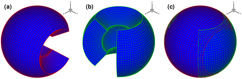
Figure 1: The Yin-Yang grids: The component grid Yin (a), Yang (b), and the overlapping grid (c).

Among the existing problems, choosing a suitable grid system is in particular critical for the implementation of any global models (not only the global force-free extrapolation) with the lower boundary as the full solar surface. Naturally one can use the spherical grid, i.e., with grid lines defined by coordinates $(r,\theta,\phi)$. However, the simplicity of a standard-spherical coordinate grid is destroyed by the problem of grid convergence and grid singularity at both poles (Usmanov, 1996; Kageyama & Sato, 2004; Feng et al., 2010). These problems severely restrict the converge speed of the full-sphere optimization code as reported by Wiegelmann (2007). Although the singularity problem can be partially resolved by excluding a small high-latitude cone, e.g., restricting the latitude within $10^{\circ}\leq\theta\leq 170^{\circ}$, it inescapably disconnects the field lines crossing over the polar region. To avoid these problems, Contopoulos et al. (2011) simply use the Cartesian grid to implement their method by taking a cubic Cartesian box to contain the whole region with the solar sphere cut out. But the Cartesian grid can not characterize precisely the Sun’s sphere surface, since the solar sphere nowhere coincides with any grid points. Thus the corresponding boundary conditions is hard to prescribe. On the other hand, the unstructured grid has been used frequently in global MHD models (Tanaka, 1994; Feng et al., 2007; Nakamizo et al., 2009) and can possibly be introduced into NLFFF extrapolation, but it costs heavily in mesh generation and management and is not suitable for solvers based on numerical difference (but may be suitable for finite element solver, e.g., the FEMQ code developed by Amari et al. (2006)). Moreover on the unstructured grid, it is difficult to implement the technique of parallelized-adaptive mesh refinement (AMR), which is an attractive tool for resolving the contradiction between the computational demand for extrapolating high-resolution/large field-of-view magnetograms and the computational resource limitations. A promising solution to the above problems is use of an overlapping spherical grid, e.g., see several types of overlapping spherical grid proposed by Usmanov (1996), Kageyama & Sato (2004), Henshaw & Schwendeman (2008) and Feng et al. (2010). In principle one can use a set of low-latitude partial-sphere grids to cover the full sphere with some patches overlapped. Certainly in such overlapping grid system, there is no pole problems and meanwhile the grid management is easy. If the component grids are carefully chosen, the overlapping patches can be minimized and only add a very small numerical overhead on the computation for data communications between the component grids. Among the overlapping grids for composing the full sphere, a so-called Yin-Yang grid (Kageyama & Sato, 2004) is a most elegant configuration with only two identical components and the overlapping region less than $7\%$ of the full sphere (see Figure 1).

Our previous work (Jiang et al., 2011; Jiang & Feng, 2012) has been devoted to a new implementation of MHD relaxation approach for NLFFF extrapolation based on the CESE numerical scheme (space-time conservation-element and solution-element scheme). We have introduced a new set of magneto-frictional-like equations with the AMR and a multigrid-like strategy for accelerating the computation and improving its convergence. The good performance and high accuracy of the code has been demonstrated by detailed comparisons with previous work by Schrijver et al. (2006) and Metcalf et al. (2008) based on several NLFFF benchmark tests, although it remains to be seen how well this method will work with real solar data. The success of the CESE-MHD-NLFFF code encourages us to extend it to spherical geometry and ultimately realize a fast and accurate way for global non-potential extrapolation of the high-resolution full-disk magnetograms from SDO. In this paper, we take the first step by developing a new code for global NLFFF extrapolation using the CESE-MHD-NLFFF method on the Yin-Yang grid. This code is assumed to be applied to force-free vector magnetograms, i.e., with the uncertainties and inconsistencies removed by some kind of preprocessing approach, e.g., that proposed by Wiegelmann et al. (2006). This is important considering that NLFFF codes generally failed to extrapolate a satisfactory force-free field when applied to non-force-free magnetogram (Metcalf et al., 2008), which is usually the case of observed data.

The remainder of the paper is organized as follows. In Section 2 we give the model equations and the numerical method including a curvilinear-version CESE-MHD scheme and its implementation in Yin-Yang grid. In Section 3 we set up two semi-analytic test cases of full-sphere NLFFF solution proposed by Low & Lou (1990). The extrapolation results and qualitative and quantitative comparisons are presented in Section 4. Finally, we draw conclusions and give some outlooks for future work in Section 5.

2 The Method

2.1 Model Equations

The basic idea of using the MHD relaxation approach to solve the force-free field is to use some kind of fictitious dissipation to drive the MHD system to an equilibrium in which all the forces can be neglected if compared to the Lorentz force and the boundary vector map is satisfied. In our previous work for NLFFF extrapolation (Jiang & Feng, 2012), a magnetic splitting form of magneto-frictional model equations is introduced as

$$\frac{\partial\rho\mathbf{v}}{\partial t}=(\nabla\times\mathbf{B}_{1})\times\mathbf{B}-\nu\rho\mathbf{v},$$

$$\frac{\partial\mathbf{B}_{1}}{\partial t}=\nabla\times(\mathbf{v}\times\mathbf{B})+\nabla(\mu\nabla\cdot\mathbf{B}_{1})-\mathbf{v}\nabla\cdot\mathbf{B}_{1},$$

$$\frac{\partial\mathbf{B}_{0}}{\partial t}=\mathbf{0},\nabla\times\mathbf{B}_{0}=\mathbf{0},\nabla\cdot\mathbf{B}_{0}=0,$$

$$\rho=|{\mathbf{B}}|^{2}+\rho_{0},\ \mathbf{B}=\mathbf{B}_{0}+\mathbf{B}_{1}.$$ (1)

In the above equation system: ${\mathbf{B}}_{0}$ is a potential field matching the normal component of the magnetogram, ${\mathbf{B}}_{1}$ is the deviation between the potential field ${\mathbf{B}}_{0}$ and the force-free field ${\mathbf{B}}$ to be solved; $\nu$ is the frictional coefficient and $\mu$ is a numerical diffusive speed of the magnetic monopole; $\rho_{0}$ is a necessary small value (e.g., $\rho_{0}=0.01$) to deal with very weak field associated with the magnetic null. The value for parameters $\nu$ and $\mu$ are respectively given by $\nu=\Delta t/\Delta x^{2}$ and $\mu=0.4\Delta x^{2}/\Delta t$, according to the time step $\Delta t$ and local grid size $\Delta x$. Merits of using the above equations include:

• Retaining explicitly the time-dependent form of the momentum equation make the magneto-frictional equation system able to be handled by modern CFD or MHD solver designed for the standard partial-differential-equation system like

  $$\frac{\partial\mathbf{U}}{\partial t}+\frac{\partial\mathbf{F({\mathbf{U}})}}{\partial x}+\frac{\partial\mathbf{G({\mathbf{U}})}}{\partial y}+\frac{\partial\mathbf{H({\mathbf{U}})}}{\partial z}=\mathbf{S}.$$ (2)

• Numerically, accuracy can be gained for solving only the deviation field ${\mathbf{B}}_{1}$ by dividing the total magnetic field $\mathbf{B}$ into two parts ($\mathbf{B}=\mathbf{B}_{0}+\mathbf{B}_{1}$) (Tanaka, 1994). Also such a splitting has a physical meaning (Priest & Forbes, 2002): potential component ${\mathbf{B}}_{0}$ arises from photospheric or sub-photospheric currents and can be regarded as invariant during a flare, whereas the non-potential component ${\mathbf{B}}_{1}$ arises from large-scale coronal currents (above the photosphere) and is the source of the flare energy.

• Any numerical magnetic monopoles $\nabla\cdot\mathbf{B}_{1}$ can be rapidly convected away with the plasma by term $-{\mathbf{v}}\nabla\cdot\mathbf{B}_{1}$ and effectively diffused out by term $\nabla(\mu\nabla\cdot\mathbf{B}_{1})$.

• Setting a pseudo-plasma density $\rho\propto|{\mathbf{B}}|^{2}$ can equalize the Alfv́en speed of the whole domain and thus accelerate the relaxation in the weak field regions.

2.2 Numerical Implementation

To solve the model equation (2.1) in spherical geometry, we employ a curvilinear version of the CESE-MHD solver proposed by Jiang et al. (2010). In this method, the governing equations written as Equation (2) are transformed from the physical space $(x,y,z)$ to a reference space $(\xi,\eta,\zeta)$ whose mapping is explicitly known $x=x(\xi,\eta,\zeta);y=y(\xi,\eta,\zeta);z=z(\xi,\eta,\zeta)$. The transformed equations are

$$\frac{\partial\hat{\mathbf{U}}}{\partial t}+\frac{\partial\hat{\mathbf{F}}}{\partial\xi}+\frac{\partial\hat{\mathbf{G}}}{\partial\eta}+\frac{\partial\hat{\mathbf{H}}}{\partial\zeta}=\hat{\mathbf{S}}$$ (3)

where

$$\left\{\begin{array}[]{lll}\hat{\mathbf{U}}=J\mathbf{U},\\ \hat{\mathbf{F}}=J(\mathbf{F}\xi_{x}+\mathbf{G}\xi_{y}+\mathbf{H}\xi_{z}),\\ \hat{\mathbf{G}}=J(\mathbf{F}\eta_{x}+\mathbf{G}\eta_{y}+\mathbf{H}\eta_{z}),\\ \hat{\mathbf{H}}=J(\mathbf{F}\zeta_{x}+\mathbf{G}\zeta_{y}+\mathbf{H}\zeta_{z}),\\ \hat{\mathbf{S}}=J\mathbf{S};\end{array}\right.$$ (9)

and $J$ is determinant of Jacobian matrix ${\mathbf{J}}$ for the mapping, i.e.,

$$\mathbf{J}=\frac{\partial(x,y,z)}{\partial(\xi,\eta,\zeta)}=\left(\begin{array}[]{ccc}x_{\xi}&x_{\eta}&x_{\zeta}\\ y_{\xi}&y_{\eta}&y_{\zeta}\\ z_{\xi}&z_{\eta}&z_{\zeta}\end{array}\right).$$ (10)

Based on this transformation, the basic idea is to map the spherical geometry of physical space to a simple rectangular grid of the reference space, in which the we can use the Cartesian CESE-MHD method to solve the transformed equations with very simple rectangular-uniform mesh. For detailed descriptions of the CESE-MHD method and its curvilinear version please refer to (Jiang et al., 2010; Feng et al., 2012).

To overcome the grid-singularity problem at both poles of the standard spherical coordinates, we use the Yin-Yang grid. As a type of overlapping grid, the Yin-Yang grid is synthesized by two identical component grids in a complemental way to cover an entire spherical surface with partial overlap on their boundaries (see Figure 1). Each component grid is a low latitude part of the latitude-longitude grid without the pole. Therefore the grid spacing on the sphere surface is quasi-uniform and the metric tensors (i.e., the matrix elements in Equation (10)) are simple and analytically known (Kageyama & Sato, 2004). In Figure 1, one component grid, say ‘Yin’ grid, is defined in the spherical coordinates by

$$|\theta-\pi/2|\leq\pi/4+\delta;|\phi-\pi|\leq 3\pi/4+\delta$$ (11)

where $\delta=1.5\Delta\theta$ is a small buffer to minimize the required overlap. The other component grid, ‘Yang’ grid, is defined by the same rule of Equation (11) but in another coordinate system that is rotated from the Yin’s, and the relation between Yin coordinates and Yang coordinates is denoted in Cartesian coordinates of each own by $(x_{e},y_{e},z_{e})=(-x_{n},z_{n},y_{n})$, where $(x_{n},y_{n},z_{n})$ is Yin’s Cartesian coordinates and $(x_{e},y_{e},z_{e})$ is Yang’s.

We then map the Yin and Yang component grids to rectangular grids by defining two mapping equations

$${\rm Yin}\left\{\begin{array}[]{l}x=e^{\xi}\sin{\theta}\cos{\phi}\\ y=e^{\xi}\sin{\theta}\sin{\phi}\\ z=e^{\xi}\cos{\theta}\end{array}\right.$$ (15)

and

$${\rm Yang}\left\{\begin{array}[]{l}x=-e^{\xi}\sin{\theta}\cos{\phi}\\ y=e^{\xi}\cos{\theta}\\ z=e^{\xi}\sin{\theta}\sin{\phi}\end{array}\right.,$$ (19)

where $(\xi,\theta,\phi)$ is the coordinates of the reference space with rectangular-uniform mesh used ($\Delta\xi=\Delta\theta=\Delta\phi$). In this definition, we have

$$\Delta r=e^{\xi+\Delta\xi}-e^{\xi}=e^{\xi}(e^{\Delta\xi}-1)\approx r\Delta\xi=r\Delta\theta$$ (20)

which means that the cells are close to regular cubes in physical space, especially at low latitudes.

The grid extent in $\xi$ is $\xi\in[0,\ln 10]$, i.e., the outer boundary is set at $r=10R_{S}$ (solar radius). The initial condition is specified by simply setting ${\mathbf{B}}_{1}={\mathbf{0}}$ and ${\mathbf{v}}={\mathbf{0}}$. The constant part ${\mathbf{B}}_{0}$ is obtained by a fast potential field solver which is developed by a combination of the spectral and the finite-difference methods (Jiang & Feng, 2012). The lower boundary condition is given by the vector magnetogram while the outer boundary is fixed with zero values of ${\mathbf{B}}_{1}$ and ${\mathbf{v}}$. In the following test cases, we focus the field extrapolation in $r\in[1,2]R_{S}$ and the objective of setting the outer boundary far beyond the extrapolation volume is to minimize the boundary effect.

On the boundaries where grids overlap, solution values on one component grid are determined by interpolation from the other. We use explicit interpolation for simplicity and efficiency in parallel computation, and the grid buffer $\delta$ is suitably chosen for enough overlap area to perform such interpolation (see Figure 1). In the reference space, standard tensor-product Lagrange interpolation (Isaacson & Keller, 1966) is used. For instance (see Figure 2 for details), the interpolation of values $f$ at the point $M(\xi_{M},\eta_{M},\zeta_{M})$ in the reference space is computed by $f(M)=\sum_{k=0}^{2}\sum_{j=0}^{2}\sum_{i=0}^{2}f(i,j,k)P_{i}^{M}(\xi)P_{j}^{M}(\eta)P_{k}^{M}(\zeta)$, where $P_{j}^{M}(x)$ is the Lagrange interpolating polynomial $P_{j}^{M}(x)=\prod_{k=0,k\neq j}^{2}\frac{x_{M}-x_{k}}{x_{j}-x_{k}}$ with $x$ being $\xi,\eta$ or $\zeta$. Note that the interpolation accuracy is of three order which is higher than the CESE solver by one order. Thus the discretization accuracy in the overlapping region will not be reduced by the interpolation. Finally, to realize the parallelization on this bi-component grids, each component grid is divided into small blocks, e.g., consisting of $8\times 8\times 8$ cells with guard-cells (one layer of ghost cells for convenience of communication between blocks), which are distributed evenly among the processors. Message-passing-interface (MPI) library is employed for data communications between the processors. The interpolation of the overlapping boundaries is dealt with in a similar way as for the intra-grid guard-cell filling and both operations are arranged to be done simultaneously. The load balancing is also considered carefully among all the processors to further improve the parallel scaling.

3 Test Case

The NLFFF model derived by Low & Lou (1990) has served as standard benchmark for many extrapolation codes (Wheatland et al., 2000; Amari et al., 2006; Schrijver et al., 2006; Valori et al., 2007; He & Wang, 2008; Jiang et al., 2011). The fields of this model are basically axially symmetric and can be represented by a second-order ordinary differential equation of $P(\mu)$ derived in spherical coordinates

$$(1-\mu^{2})\frac{d^{2}P}{d\mu^{2}}+n(n+1)P+a^{2}\frac{1+n}{n}P^{1+2/n}=0$$ (21)

where $n$ and $a$ are constants and $\mu=\cos\theta$. With boundary conditions of $P=0$ at $\mu=-1,1$, the solution $P$ of Equation (21) is uniquely determined by two eigenvalues, $n$ and its number of nodes $m$ (Low & Lou, 1990; Amari et al., 2006). The magnetic fields are then given by

$$B_{r}=\frac{1}{r^{2}\sin\theta}\frac{\partial A}{\partial\theta},B_{\theta}=-\frac{1}{r\sin\theta}\frac{\partial A}{\partial r},B_{\phi}=\frac{1}{r\sin\theta}Q$$ (22)

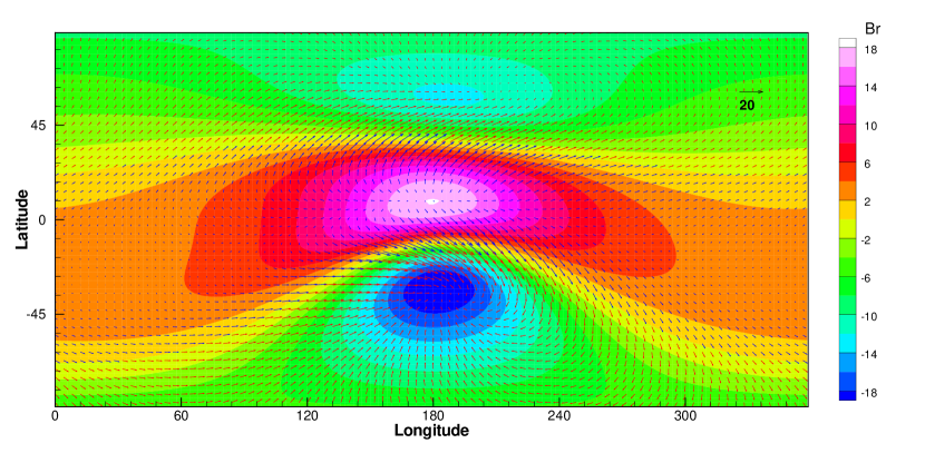
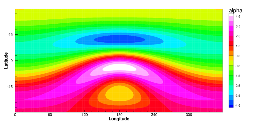
Figure 3: Vector map (upper) and $\alpha$ distribution (bottom) of CASE LL1. In the vector map, the contours represent $B_{r}$ and the tangential field $(B_{\phi},B_{\theta})$ is shown by the vectors with blue color in positive $B_{r}$ region and red in negative $B_{r}$ region.

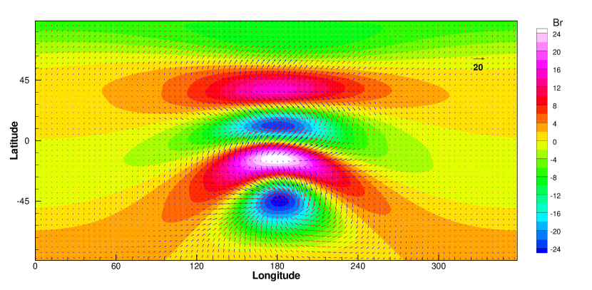
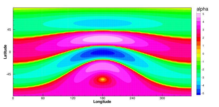
Figure 4: Same as Figure 3 but for CASE LL2.

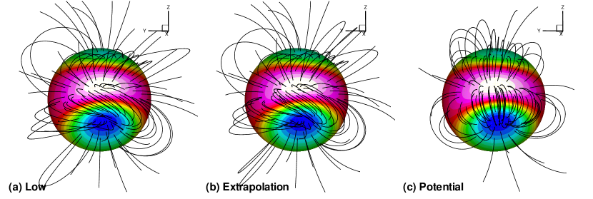
Figure 5: CASE LL1: 3D magnetic field lines with contour of $B_{r}$ on the photosphere surface, (a) Low & Lou’s solution; (b) the extrapolation result; (c) the initial potential field.

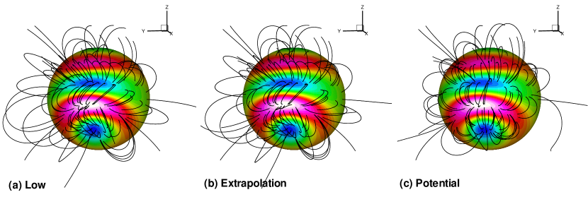
Figure 6: Same as Figure 5 but for CASE LL2.

where $A=P(\mu)/r^{n}$ and $Q=aA^{1+1/n}$. The fields are axisymmetric in spherical coordinates (i.e., invariant in $\phi$ direction) with a point source at the origin. To avoid such obvious symmetry in the full-3D extrapolation test, we locate the point source with $0.3R_{S}$ offset to the center of the computational volume and deviate the axis of symmetry with the $z$–axis by $\Phi=\pi/10$ (the length unit of the above equations is the solar radius $R_{S}$). We present two test cases with eigenvalues of $n=1,m=1$ (hereafter referred to as CASE LL1) and $n=3,m=1$ (CASE LL2) respectively. Both cases are performed on the same resolution of $90\times 180$ grids in $\theta$–$\phi$ plane and $r\in[1,2]R_{S}$. The synoptic maps of the field and the force-free parameter $\alpha$ at the bottom of the solutions are shown in Figures 3 and 4 and the 3D field lines are shown in panel (a) of Figures 5 and 6. It should be remarked that these magnetograms do not represent the real magnetic distributions of the photosphere but only be used for the purpose of testing our code. As can be seen, the $\alpha$ distribution of CASE LL2 is more inhomogeneous than that of CASE LL1, which means that CASE LL2 is more nonlinear. We note that CASE LL1 is very similar to test cases used by Wiegelmann (2007) and Tadesse et al. (2009) while CASE LL2 is more difficult than tests in their works.

Before inputting the vector maps in the NLFFF code, we made some consistency checks for the maps. If a vector map is used for a force-free extrapolation, some necessary conditions have to be fulfilled (Aly, 1989; Sakurai, 1989; Tadesse et al., 2009). For clarification we repeat here these conditions from Tadesse (2011) where a detailed derivation of the condition formula is given. First of all the net magnetic flux must be in balance, i.e.,

$$\int_{S}B_{r}{\ \mathrm{d}}s=0$$ (23)

where $S$ represents the whole sphere. Secondly the total force on the boundary has to vanish, which can be expressed in spherical coordinates as

$$\mathcal{F}_{1}=\int_{S}\left[\frac{1}{2}(B_{\theta}^{2}+B_{\phi}^{2}-B_{r}^{2})\sin\theta\cos\phi-B_{r}B_{\theta}\cos\theta\cos\phi+B_{r}B_{\phi}\sin\phi\right]{\ \mathrm{d}}s=0;$$

$$\mathcal{F}_{2}=\int_{S}\left[\frac{1}{2}(B_{\theta}^{2}+B_{\phi}^{2}-B_{r}^{2})\sin\theta\sin\phi-B_{r}B_{\theta}\cos\theta\sin\phi-B_{r}B_{\phi}\cos\phi\right]{\ \mathrm{d}}s=0;$$

$$\mathcal{F}_{3}=\int_{S}\left[\frac{1}{2}(B_{\theta}^{2}+B_{\phi}^{2}-B_{r}^{2})\cos\theta+B_{r}B_{\theta}\sin\theta\right]{\ \mathrm{d}}s=0.$$ (24)

Thirdly the total torque on the boundary vanishes, i.e.,

$$\mathcal{T}_{1}=\int_{S}B_{r}(B_{\phi}\cos\theta\cos\phi+B_{\theta}\sin\phi){\ \mathrm{d}}s=0;$$

$$\mathcal{T}_{2}=\int_{S}B_{r}(B_{\phi}\cos\theta\sin\phi-B_{\theta}\cos\phi){\ \mathrm{d}}s=0;$$

$$\mathcal{T}_{3}=\int_{S}B_{r}B_{\phi}\sin\theta{\ \mathrm{d}}s=0.$$ (25)

To quantify the quality of the synthetic full-disk magnetograms with respect to the above criteria, we compute three parameters, i.e., the flux balance parameter

$$\epsilon_{\rm flux}=\frac{\int_{S}B_{r}{\ \mathrm{d}}s}{\int_{S}|B_{r}|{\ \mathrm{d}}s},$$ (26)

the force balance parameter

$$\epsilon_{\rm force}=\frac{|\mathcal{F}_{1}|+|\mathcal{F}_{2}|+|\mathcal{F}_{3}|}{E_{B}}$$ (27)

and the torque balance parameter

$$\epsilon_{\rm torque}=\frac{|\mathcal{T}_{1}|+|\mathcal{T}_{2}|+|\mathcal{T}_{3}|}{E_{B}}$$ (28)

where $E_{B}=\int_{S}(B_{r}^{2}+B_{\theta}^{2}+B_{\phi}^{2}){\ \mathrm{d}}s$. For the above cases, the three parameters are $(-7.117\times 10^{-4},1.181\times 10^{-4},6.313\times 10^{-6})$ and $(-1.028\times 10^{-3},5.458\times 10^{-4},7.379\times 10^{-5})$ respectively, which shows that these maps are ideally consistent with the force-free model.

4 Results

In this section, we present the results of extrapolation and compare them with their original solutions qualitatively and quantitatively. As usual, the quantitative comparison is performed by computing a suite of metrics (also referred to as figures of merit), which are listed as follows:

• the vector correlation $C_{\rm vec}$

  $$C_{\rm vec}\equiv\sum_{i}\mathbf{B}_{i}\cdot\mathbf{b}_{i}/(\sum_{i}|\mathbf{B}_{i}|^{2}\sum_{i}|\mathbf{b}_{i}|^{2}),$$ (29)

• the Cauchy-Schwarz inequality $C_{\rm CS}$

  $$C_{\rm CS}\equiv\frac{1}{M}\sum_{i}\frac{\mathbf{B}_{i}\cdot\mathbf{b}_{i}}{|\mathbf{B}_{i}||\mathbf{b}_{i}|},$$ (30)

• the normalized and mean vector error $E_{\rm n}^{\prime}$, $E_{\rm m}^{\prime}$

  $$E_{\rm n}\equiv\sum_{i}|\mathbf{b}_{i}-\mathbf{B}_{i}|/\sum_{i}|\mathbf{B}_{i}|;E_{\rm n}^{\prime}=1-E_{\rm n},$$ (31)

  $$E_{\rm m}\equiv\frac{1}{M}\sum_{i}\frac{|\mathbf{B}_{i}-\mathbf{b}_{i}|}{|\mathbf{B}_{i}|};E_{\rm m}^{\prime}=1-E_{\rm m},$$ (32)

• the magnetic energy ratio $\epsilon$

  $$\epsilon=\frac{\sum_{i}|{\mathbf{b}}_{i}|^{2}}{\sum_{i}|{\mathbf{B}}_{i}|^{2}},$$ (33)

where ${\mathbf{B}}_{i}$ and ${\mathbf{b}}_{i}$ denote the Low & Lou solution and the extrapolated field, respectively, $i$ denotes the indices of the grid points and $M$ is the total number of grid points involved. It is also important to measure the ratio of the total energy to the potential energy

$$E/E_{\rm pot}=\frac{\sum_{i}|{\mathbf{B}}_{i}|^{2}}{\sum_{i}|({\mathbf{B}}_{\rm pot})_{i}|^{2}}$$ (34)

to study the free energy budget for realistic coronal field.

We also calculate another four metrics to measure the force-freeness and divergence-freeness of the results. They are the current-weighted sine metric CWsin

$${\rm CWsin}\equiv\frac{\sum_{i}|\mathbf{J}_{i}|\sigma_{i}}{\sum_{i}|\mathbf{J}_{i}|};\sigma_{i}=\frac{|\mathbf{J}_{i}\times\mathbf{B}_{i}|}{|\mathbf{J}_{i}||\mathbf{B}_{i}|},$$ (35)

the divergence metric $\langle|f_{i}|\rangle$

$$\langle|f_{i}|\rangle=\frac{1}{M}\sum_{i}\frac{(\nabla\cdot\mathbf{B})_{i}}{6|{\mathbf{B}}_{i}|/\Delta x},$$ (36)

and the $E_{\nabla\cdot\mathbf{B}}$ and $E_{\nabla\times\mathbf{B}}$

$$E_{\nabla\cdot\mathbf{B}}=\frac{1}{M}\sum_{i}\frac{|\mathbf{B}_{i}(\nabla\cdot\mathbf{B})_{i}|}{|\nabla(|{\mathbf{B}}|^{2}/2)_{i}|};$$

$$E_{\nabla\times\mathbf{B}}=\frac{1}{M}\sum_{i}\frac{|{\mathbf{J}}_{i}\times{\mathbf{B}}_{i}|}{|\nabla(|{\mathbf{B}}|^{2}/2)_{i}|}.$$ (37)

All the above metrics have been described in detail in our previous work Jiang & Feng (2012) and thus will not be repeated here.

4.1 Qualitative Comparison

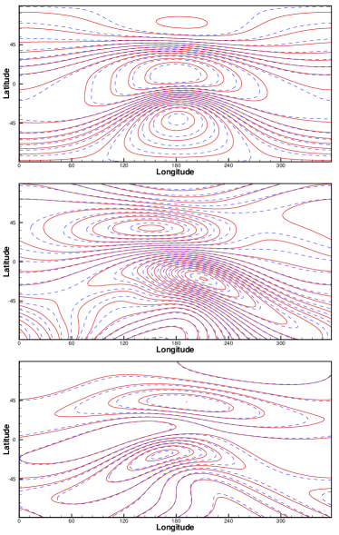
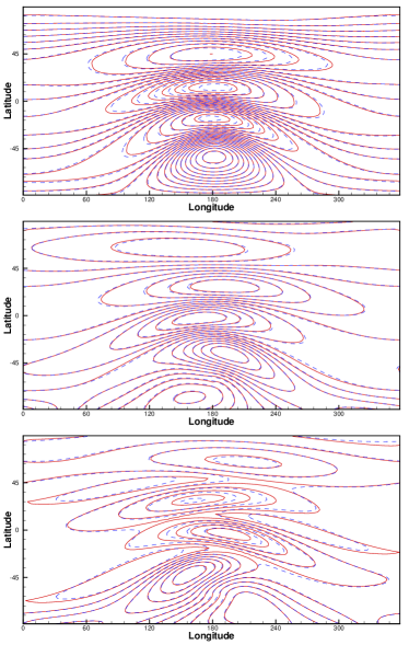
Figure 7: Contour map comparison of the Low & Lou’s solution (solid lines) and extrapolation solution (dashed lines) at $r=1.5R_{S}$ for $B_{r}$ (top), $B_{\theta}$ (middle) and $B_{\phi}$ (bottom). Left column is for CASE LL1 and right for CASE LL2.

In Figures 5 and 6, we present a side-by-side comparisons of the extrapolation results with the Low & Lou models and the potential fields by plotting the 3D field configurations. For each cases the field lines are traced from the same set of footpoints on the photosphere. A good agreement between our extrapolation results and the original Low & Lou solutions can be seen from the highly similarity of most of the field lines. The basic difference between the extrapolated fields and the potential fields is the shearing, which is reconstructed by the bottom-boundary-driving process exerted on the initial un-sheared potential fields. By placing the outer boundary far away enough, we can make most of the field lines move freely in the volume, which thus is helpful for the relaxation of the field lines. Figure 7 compares the field values of the $r=1.5R_{S}$ surface by plotting the contours of the reference solutions (solid lines) and the extrapolation (dashed lines) on the same figure. As can be seen, contours lines of the fields from the reference solution and the extrapolation almost overlapped with each other.

4.2 Quantitative Comparison

Quantitative metrics shown in Table 1 and 2 demonstrate good performance of the code. In these tables, we present results of the full sphere with $r\in[1,2]R_{S}$ and more lower region $r\in[1,1.5]R_{S}$. For both cases results of the vector correlation $C_{\rm vec}$ and $C_{\rm CS}$ are extremely close to the reference values, showing a perfect matching of the vector direction. Results of vector error $E_{\rm n}^{\prime}$ and $E_{\rm m}^{\prime}$ also score close to $1$ (even the error of most sensitive metric $E_{\rm m}^{\prime}$ is smaller than $10\%$), while the potential solutions have results of only $\sim 0.5$. This is very encouraging, since in previously reported tests of Cartesian or spherical NLFFF extrapolation code with only photospheric boundary provided, e.g., done by Schrijver et al. (2006); Valori et al. (2007); Wiegelmann (2007); Tadesse et al. (2009), results with $E_{\rm m}^{\prime}>0.9$ are rarely achieved. These two metrics show that the original solutions are reconstructed with very high accuracy. Finally, the energy content of the non-potential fields, a critical parameter from the extrapolation used to calculate the energy budget in solar eruptions, is also well reproduced (with errors under several percents). By comparison of the metrics, we find that accuracy of the lower region is even higher than the full region, which means the strong fields are extrapolated better than the upper-region weak fields. In real solar fields, only the lower part of the corona is close to force-free while the upper corona is no more force-free because of the expansion of hot plasma (Gary, 2001). Thus to extrapolate the lower-region fields more close to the original force-free solution than the upper-region fields is consistent with the real solar conditions.

Table 3 gives the metrics measuring force-freeness and divergence-freeness of the fields, which are rather small and close to the level of discretization error. Unlike the first two metrics (CWsin and $\langle|f_{i}|\rangle$) which mainly characterize the geometric properties of the field, metrics $E_{\nabla\times\mathbf{B}}$ and $E_{\nabla\cdot\mathbf{B}}$ are introduced to measure the physical effect of the residual divergence and Lorentz forces on the system in the actual numerical computation (Jiang & Feng, 2012). This is important when checking the NLFFF solution if it is used to initiate any full-MHD simulations. Of the present extrapolation results, the residual forces are less than one percent of the magnetic-pressure force.

4.3 Convergence Study

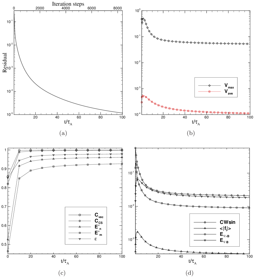
Figure 8: CASE LL1: The history of the relaxation to force-free equilibrium. (a) Evolution of residual ${\rm res}({\mathbf{B}}_{1})$ with time (and the iteration steps); (b) evolution of the maximum and average velocity; and (c), (d) evolution of the metrics.

We finally give a study of convergence of the extrapolation. In Figure 8 and 9 we show how the system relaxes and reaches its final force-free equilibrium by plotting the temporal evolution of several parameters, including the residual of field ${\mathbf{B}}_{1}$

$${\rm res}^{n}({\mathbf{B}}_{1})=\sqrt{\frac{1}{3}\sum_{\delta=x,y,z}\frac{\sum_{i}(B_{i\delta}^{n}-B_{i\delta}^{n-8})^{2}}{\sum_{i}(B_{i\delta}^{n})^{2}}}$$ (38)

(where $n$ denotes the iteration steps), the maximum and average velocity, and the nine metrics described above. The system converged very fast from a initial residual of $>10^{-1}$ to value $\sim 10^{-5}$ with time of $100\tau_{A}$ (about $6000\sim 8000$ iteration steps, see panel (a) of the figures). The evolution of the plasma velocity indicates that initially (1) the system is driven away from the starting ${\mathbf{v}}=0$ state and then (2) by the relaxation process a static equilibrium is reached as expected with a rather small residual velocity which is only on the order of the numerical error $O(\Delta x^{2})$ of the CESE solver. All the metrics plotted in the figures converged after $40\tau_{A}$ (less than 2000 iteration steps), when the residual is on the order of $10^{-4}$, and the convergence speed of CASE LL2 is even faster than CASE LL1. Note that the metrics $\langle|f_{i}|\rangle$ and $E_{\nabla\cdot\mathbf{B}}$, like the plasma velocity, first climbs to a relatively high level (see panel (d)) and then drops to the level of discretization errors. In principle the divergence-free constraint of ${\mathbf{B}}$ should be fulfilled throughout the evolution, at least close to level of discretization error. However, an ideally dissipationless induction equation Equation (2.1) with divergence-free constraint can preserve the magnetic connectivity, which makes the topology of the magnetic field unchangeable (Wiegelmann, 2008) unless a finite resistivity is included to allow the reconnection and changing of the magnetic topology (Roumeliotis, 1996). In the present implementation in which no resistivity is included in the induction equation, an allowing of high values in $\nabla\cdot\mathbf{B}$ in the initial evolution process (indicated by the climb of metric $\langle|f_{i}|\rangle$) may provide some freedom for changes in the magnetic topology (also note that a numerical diffusion can help topology adjustment).

Besides the extrapolation accuracy, the computing time also matters for a practical use of the NLFFF code. In this present tests, the size of the Yin-Yang grid is equivalent to $80\times 90\times 180$ in ordinary spherical grid. The computation is completed by less than 2 hours using $32$ processors of Intel Xeon CPU E5450 (3.00GHz). In practical applications, the computing time can be further reduced considering that it is not necessary to evolve the system to $100\tau_{\rm A}$.

5 Conclusions

In this work we present a new code for NLFFF extrapolation of the global corona. The method is implemented by installing the previous code CESE-MHD-NLFFF in the Cartesian geometry onto a Yin-Yang spherical grid. By this grid system, we can incorporate intrinsically the full-sphere computation and avoid totally the problems involved with the spherical poles. The boundary conditions are only specified on the bottom sphere and free of any lateral-boundary information. We have examined the performance of this newly developed code using two test cases of the classic semi-analytic force-free fields by Low & Lou (1990). We show that the code runs fast and achieves a good accuracy with the extrapolation solution very close to the reference field and the force-freeness and divergence-freeness constraints well fulfilled.

We note that the success of extrapolating the model solutions (i.e., the ideal force-free test cases) does not necessarily indicate successful applications to the real solar data, which contains various inconsistencies and uncertainties. A practicable solution to this issue may be attributed to some preprocessing methods as developed by Wiegelmann et al. (2006) and Fuhrmann et al. (2007) or more realistic MHD model focused on the photosphere-chromosphere interface with atmosphere stratification. For another important issue, reconstruction that need to be performed with much larger field of view (to more entirely characterize the currents between ARs and high over the AR) and with higher spatial resolution (to capture the fine critical structures such magnetic null point) is severely limited by the computational capability. Application with grid of about $500^{3}$ pixels is almost the upper limit for computational capability of most recently developed or updated codes. This is rather unsatisfied if considering extrapolation with the $4096\times 4096$ SDO/HMI magnetograms. This issue can be resolved promisingly via combining the global extrapolation code with the adaptive mesh refinement, according to the intrinsic characteristics of the solar magnetic field in which the active regions represents only a small fraction of the whole surface. By the AMR technique, one can take focus on local corona, e.g., some active regions in the context of global extrapolation with the corresponding high-resolution vector magnetograms embedded in a low-resolution global vector or LoS map, as exemplified by Figure 10. In this figure , mesh for the active regions are refined with three more grid levels than the background full-sphere grid (a block-AMR algorithm (Powell et al., 1999) is used and the ratio of resolutions between the grid levels is two). The grid structure can be dynamically adjusted during the MHD-relaxation process to capture the strong currents and important magnetic structures (e.g., flux ropes) by designing carefully the AMR refinement criteria. Our future work will include performing more stringent testing of the code and installation of the code on AMR grid for practical application to SDO/HMI data.

Model	$C_{\rm vec}$	$C_{\rm CS}$	$E_{\rm n}^{\prime}$	$E_{\rm m}^{\prime}$	$\epsilon$	$E/E_{\rm pot}$
For $r\in[1,2]R_{S}$
Low	1	1	1	1	1	1.1741
Extrapolation	0.9995	0.9974	0.9609	0.9269	0.9783	1.1486
Potential	0.8595	0.8204	0.5261	0.4641	0.8517	1
For $r\in[1,1.5]R_{S}$
Low	1	1	1	1	1	1.1390
Extrapolation	0.9998	0.9995	0.9772	0.9668	0.9851	1.1220
Potential	0.8620	0.8236	0.5441	0.5013	0.8780	1

Table 1: CASE LL1: Results of the metrics.

Model	$C_{\rm vec}$	$C_{\rm CS}$	$E_{\rm n}^{\prime}$	$E_{\rm m}^{\prime}$	$\epsilon$	$E/E_{\rm pot}$
For $r\in[1,2]R_{S}$
Low	1	1	1	1	1	1.1042
Extrapolation	0.9999	0.9965	0.9807	0.9456	1.0061	1.1110
Potential	0.9049	0.8013	0.5733	0.4515	0.9056	1
For $r\in[1,1.5]R_{S}$
Low	1	1	1	1	1	1.0999
Extrapolation	0.9999	0.9997	0.9864	0.9810	1.0063	1.1068
Potential	0.9055	0.8529	0.5861	0.5174	0.9092	1

Table 2: CASE LL2: Results of the metrics.

Case	CWsin	$\langle|f_{i}|\rangle$	$E_{\nabla\times\mathbf{B}}$	$E_{\nabla\cdot\mathbf{B}}$
LL1	$2.11\times 10^{-2}$	$3.73\times 10^{-4}$	$9.04\times 10^{-3}$	$1.83\times 10^{-2}$
LL2	$2.68\times 10^{-2}$	$4.09\times 10^{-4}$	$5.94\times 10^{-3}$	$7.64\times 10^{-3}$

Table 3: Results for the metrics measuring the force-freeness and divergence-freeness.

Figure 2: Interpolation of the point $M$ in the reference space: $M$ represents a mesh point on the overlapping boundary, for example, of Yin grid, then the twenty-seven ($3^{3}$) nodes denote the Yang’s inner mesh points that are closest to $M$.

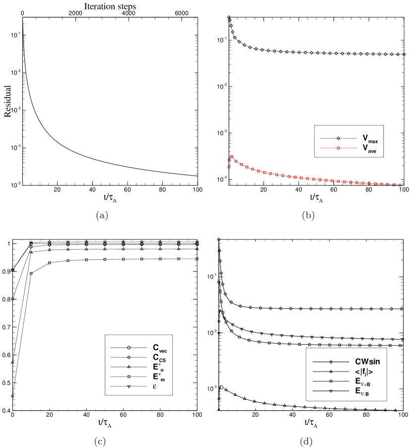
Figure 9: Same as Figure 8 but for CASE LL2.

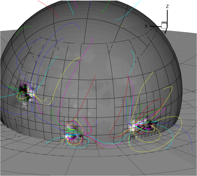
Figure 10: A example of global extrapolation with AMR grid. The sphere represents the photosphere with grid structure outlined by the black lines (note that here each mesh cell represent one grid block). The color lines represent the magnetic field lines and the grey image represents the radial field $B_{r}$. A slice of $z=-0.3$ is plotted to show the radial mesh structure. Note that the high-resolution blocks are clustered around the active regions.

References

- Aly (1989) Aly, J. J. 1989, Sol. Phys., 120, 19
- Amari et al. (1997) Amari, T., Aly, J. J., Luciani, J. F., Boulmezaoud, T. Z., & Mikic, Z. 1997, Sol. Phys., 174, 129
- Amari et al. (2006) Amari, T., Boulmezaoud, T. Z., & Aly, J. J. 2006, A&A, 446, 691
- Bobra et al. (2008) Bobra, M. G., van Ballegooijen, A. A., & DeLuca, E. E. 2008, ApJ, 672, 1209
- Contopoulos et al. (2011) Contopoulos, I., Kalapotharakos, C., & Georgoulis, M. K. 2011, Sol. Phys., 269, 351
- DeRosa et al. (2009) DeRosa, M. L., Schrijver, C. J., Barnes, G., Leka, K. D., Lites, B. W., Aschwanden, M. J., Amari, T., Canou, A., McTiernan, J. M., Régnier, S., Thalmann, J. K., Valori, G., Wheatland, M. S., Wiegelmann, T., Cheung, M. C. M., Conlon, P. A., Fuhrmann, M., Inhester, B., & Tadesse, T. 2009, ApJ, 696, 1780
- Feng et al. (2007) Feng, X., Zhou, Y., & Wu, S. T. 2007, ApJ, 655, 1110
- Feng et al. (2012) Feng, X. S., Yang, L. P., Xiang, C. Q., Jiang, C. W., Ma, X. P., Wu, S. T., Zhong, D. K., & Zhou, Y. F. 2012, Sol. Phys., In press
- Feng et al. (2010) Feng, X. S., Yang, L. P., Xiang, C. Q., Wu, S. T., Zhou, Y. F., & Zhong, D. K. 2010, ApJ, 723, 300
- Fuhrmann et al. (2007) Fuhrmann, M., Seehafer, N., & Valori, G. 2007, A&A, 476, 349
- Gary & Hurford (1994) Gary, D. E. & Hurford, G. J. 1994, ApJ, 420, 903
- Gary (2001) Gary, G. A. 2001, Sol. Phys., 203, 71
- He & Wang (2006) He, H. & Wang, H. 2006, MNRAS, 369, 207
- He & Wang (2008) —. 2008, J. Geophys. Res., 113, 5
- Henshaw & Schwendeman (2008) Henshaw, W. D. & Schwendeman, D. W. 2008, J. Comput. Phys., 227, 7469
- Isaacson & Keller (1966) Isaacson, E. & Keller, H. B. 1966, Analysis of numerical methods (John Wiley & Sons)
- Jiang & Feng (2012) Jiang, C. & Feng, X. 2012, ApJ, 749, 135
- Jiang et al. (2011) Jiang, C., Feng, X., Fan, Y., & Xiang, C. 2011, ApJ, 727, 101
- Jiang & Feng (2012) Jiang, C. W. & Feng, X. S. 2012, Sol. Phys., Under review
- Jiang et al. (2010) Jiang, C. W., Feng, X. S., Zhang, J., & Zhong, D. K. 2010, Sol. Phys., 267, 463
- Kageyama & Sato (2004) Kageyama, A. & Sato, T. 2004, Geochemistry, Geophysics, Geosystems, 5, 9005
- Lin et al. (2004) Lin, H., Kuhn, J. R., & Coulter, R. 2004, ApJ, 613, L177
- Low & Lou (1990) Low, B. C. & Lou, Y. Q. 1990, ApJ, 352, 343
- McClymont et al. (1997) McClymont, A. N., Jiao, L., & Mikic, Z. 1997, Sol. Phys., 174, 191
- Metcalf et al. (2008) Metcalf, T. R., DeRosa, M. L., Schrijver, C. J., Barnes, G., van Ballegooijen, A. A., Wiegelmann, T., Wheatland, M. S., Valori, G., & McTtiernan, J. M. 2008, Sol. Phys., 247, 269
- Nakamizo et al. (2009) Nakamizo, A., Tanaka, T., Kubo, Y., Kamei, S., Shimazu, H., & Shinagawa, H. 2009, Journal of Geophysical Research (Space Physics), 114, A07109
- Powell et al. (1999) Powell, K. G., Roe, P. L., Linde, T. J., Gombosi, T. I., & de Zeeuw, D. L. 1999, J. Comput. Phys., 154, 284
- Priest & Forbes (2002) Priest, E. R. & Forbes, T. G. 2002, A&A Rev., 10, 313
- Roumeliotis (1996) Roumeliotis, G. 1996, ApJ, 473, 1095
- Sakurai (1989) Sakurai, T. 1989, Space Sci. Rev., 51, 11
- Savcheva & van Ballegooijen (2009) Savcheva, A. & van Ballegooijen, A. 2009, ApJ, 703, 1766
- Schrijver et al. (2006) Schrijver, C. J., De Rosa, M. L., Metcalf, T. R., Liu, Y., McTiernan, J., Régnier, S., Valori, G., Wheatland, M. S., & Wiegelmann, T. 2006, Sol. Phys., 235, 161
- Solanki et al. (2006) Solanki, S. K., Inhester, B., & Schüssler, M. 2006, Reports on Progress in Physics, 69, 563
- Su et al. (2009a) Su, Y., van Ballegooijen, A., Lites, B. W., Deluca, E. E., Golub, L., Grigis, P. C., Huang, G., & Ji, H. 2009a, ApJ, 691, 105
- Su et al. (2009b) Su, Y., van Ballegooijen, A., Schmieder, B., Berlicki, A., Guo, Y., Golub, L., & Huang, G. 2009b, ApJ, 704, 341
- Tadesse (2011) Tadesse, T. 2011, PhD thesis, Max Planck Institute for Solar System Research
- Tadesse et al. (2009) Tadesse, T., Wiegelmann, T., & Inhester, B. 2009, A&A, 508, 421
- Tadesse et al. (2011) Tadesse, T., Wiegelmann, T., Inhester, B., & Pevtsov, A. 2011, A&A, 527, A30
- Tadesse et al. (2012) —. 2012, Sol. Phys., 277, 119
- Tanaka (1994) Tanaka, T. 1994, J. Comput. Phys., 111, 381
- Usmanov (1996) Usmanov, A. V. 1996, in American Institute of Physics Conference Series, Vol. 382, American Institute of Physics Conference Series, ed. D. Winterhalter, J. T. Gosling, S. R. Habbal, W. S. Kurth, & M. Neugebauer, 141–144
- Valori et al. (2007) Valori, G., Kliem, B., & Fuhrmann, M. 2007, Sol. Phys., 245, 263
- van Ballegooijen (2004) van Ballegooijen, A. A. 2004, ApJ, 612, 519
- Wang et al. (2001) Wang, H., Chae, J., Yurchyshyn, V., Yang, G., Steinegger, M., & Goode, P. 2001, ApJ, 559, 1171
- Wheatland et al. (2000) Wheatland, M. S., Sturrock, P. A., & Roumeliotis, G. 2000, ApJ, 540, 1150
- Wiegelmann (2007) Wiegelmann, T. 2007, Sol. Phys., 240, 227
- Wiegelmann (2008) —. 2008, J. Geophys. Res., 113, 3
- Wiegelmann et al. (2006) Wiegelmann, T., Inhester, B., & Sakurai, T. 2006, Sol. Phys., 233, 215
- Yan & Li (2006) Yan, Y. & Li, Z. 2006, ApJ, 638, 1162