Discrete Morse functions for graph configuration spaces

Abstract

We present an alternative application of discrete Morse theory for two-particle graph configuration spaces. In contrast to previous constructions, which are based on discrete Morse vector fields, our approach is through Morse functions, which have a nice physical interpretation as two-body potentials constructed from one-body potentials. We also give a brief introduction to discrete Morse theory. Our motivation comes from the problem of quantum statistics for particles on networks, for which generalised versions of anyon statistics can appear.

1 Introduction

In non-relativistic quantum mechanics a quantum system is described by a wavefunction which fulfills the Schrödinger equation. Moreover, for a system of many identical particles the additional symmetrization (for bosons) or antisymmetrization (for fermions) of the wavefunction is imposed. Around a quarter-century ago Souriau [1], Leinaas and Myrheim [2], and subsequently Wilczek [3], noticed that for identical particles confined to two dimensions there are other possibilities, namely one can have exotic quantum statistics, aka anyons. Recently [5] Harrison, Keating and Robbins (see also [6]) discussed the quantum abelian statistics of two indistinguishable spinless particles on a quantum graph. They found that in spite of the fact that the model is locally one-dimensional, anyon statistics are present. Moreover, they noticed that at least a priori there is a possibility of having more than one statistics phase. The analysis described in [5] is simplified by considering combinatorial, rather than metric, graphs i.e. many-particle tight-binding models. It was shown in [7] that under some further assumptions, which are specified in section 2.2, many-particle combinatorial graphs have the same topological properties as their metric counterparts and hence combinatorial graphs are equivalent to metric ones from the point of view of quantum statistics. As discussed in section 2, the first homology group of an appropriate configuration space is related to quantum statistics [4, 5].

Recently there has been significant progress in understanding topological properties of configuration spaces of many particles on metric graphs [9, 10]. This was enabled by the foundational development of discrete Morse theory by Forman during the late 1990’s [11]. This theory reduces the calculation of homology groups to an essentially combinatorial problem, namely the construction of certain discrete Morse functions, or equivalently discrete gradient vector fields. Using this idea Farley and Sabalka [9] gave a recipe for the construction of such a discrete gradient vector field [9] on many-particle graphs and classified the first homology groups for tree graphs. In 2011 Ko and Park [10] significantly extended these results to arbitrary graphs by incorporating graph-theoretic theorems concerning the decomposition of a graph into its two and three-connected components.

In the current paper we give an alternative application of discrete Morse theory for two-particle graph configuration spaces. In contrast to the construction given in [9], which is based on discrete Morse vector fields, our approach is through discrete Morse functions. Our main goal is to provide an intuitive way of constructing a discrete Morse function and hence a discrete Morse gradient vector field. The central object of the construction is the ‘trial Morse’ function. It may be understood as two-body potential constructed from one-body potential, a perspective which is perhaps more natural and intuitive from a physics point of view. Having a perfect Morse function $f_{1}$ on a graph $\Gamma$ we treat it as a one-body potential. The value of the trial Morse function at each point of a two-particle configuration space is the sum of the values of $f_{1}$ corresponding to the two particles positions in $\Gamma$. The trial Morse function is typically not a Morse function, i.e. it might not satisfy some of the relevant conditions. Nevertheless, we find that it is always possible to modify it and obtain a proper Morse function out of it. In fact, the trial Morse function is not ‘far’ from being a Morse function and the number of cells at which it needs fixing is relatively small. Remarkably, this simple idea leads to similar results as those obtained in [9]. We demonstrate it in Section 5 by calculating two simple examples. We find that in both cases the trial Morse function has small defects which can be easily removed and a proper Morse function is obtained. The corresponding discrete Morse vector field is equivalent to the one stemming from the Farley and Sabalka method [9]. As is shown in Section 7, it is always possible to get rid of defects of the trial Morse function. The argument is rather technical. However, since the problem is of a certain combinatorial complexity we believe it cannot be easily simplified. We describe in details how the final result, i.e set of discrete Morse functions along with rules for identifying the critical cells and constructing the boundary map of the associated Morse complex, is built in stages from this simple idea. Our main purpose is hence to present an approach which we believe is conceptually simple and physically natural. It would be interesting to check if the presented constructions can give any simplification in understanding the results of [10] but we do not pursue this here.

The paper is organized as follows. In section 2 we discuss the relation between quantum statistics and the first homology group of a configuration space. In section 3 we give a brief introduction to discrete Morse theory. Then in sections 4 and 5, for two examples we present a definition of a ‘trial’ Morse function $\tilde{f}_{2}$ for two-particle graph configuration space. We notice that the trial Morse function typically does not satisfy the conditions required of a Morse function according to Forman’s theory. Nevertheless, we show in Section 7 that with small modifications, which we explicitly identify, the trial Morse function can be transformed into a proper Morse function. Since the number of critical cells and hence the size of the associated Morse complex is small compared with the size of configuration space the calculation of homology groups are greatly simplified. The technical details of the proofs are given in the Appendix. In section 6 we discuss more specifically how the techniques of discrete Morse theory apply to the problem of quantum statistics on graphs.

2 Quantum statistics and the fundamental group

Symmetrization (for bosons) and anti-symmetrization (for fermions) of the Hilbert space of indistinguishable particles is typically introduced as an additional postulate of non-relativistic quantum mechanics. More precisely, for indistinguishable particles the Hilbert space of a composite, $n$-partite system is not the tensor product of the single-particle Hilbert space but rather,

1. the antisymmetric part of the tensor product, for fermions,

2. the symmetric part of the tensor product, for bosons.

In terms of the wave function in the position representation this translates to

$$\Psi(x_{1},\ldots,x_{i},\ldots,x_{j},\ldots x_{n})=\Psi(x_{1},\ldots,x_{j},\ldots,x_{i},\ldots x_{n})\,\,\,\,\,\mathrm{for}\,\,\mathrm{bosons},$$

$$\Psi(x_{1},\ldots,x_{i},\ldots,x_{j},\ldots x_{n})=-\Psi(x_{1},\ldots,x_{j},\ldots,x_{i},\ldots x_{n})\,\,\,\,\,\mathrm{for}\,\,\mathrm{fermions},$$

i.e., when two fermions are exchanged the sign of wave function changes and for bosons it stays the same.

It was first noticed by Souriau [1], and subsequently by Leinaas and Myrheim [2] that this additional postulate can be understood in terms of topological properties of the classical configuration space of indistinguishable particles.

Let us denote by $M$ the one-particle classical configuration space (e.g., an $m$-dimensional manifold) and by

$$F_{n}(M)=\{(x_{1},\,x_{2},\ldots,\,x_{n})\,:x_{i}\in X,\,x_{i}\neq x_{j}\},$$ (1)

the space of $n$ distinct points in $M$. The $n$-particle configuration space is defined as an orbit space

$$C_{n}(M)=\nicefrac{{F_{n}(M)}}{{S_{n}}},$$ (2)

where $S_{n}$ is the permutation group of $n$ elements and the action of $S_{n}$ on $F_{n}(M)$ is given by

$$\sigma(x_{1}\,,\ldots\,x_{2})=(x_{\sigma(1)}\,,\ldots\,x_{\sigma(2)}),\,\,\,\,\forall\sigma\in S_{n}.$$ (3)

Any closed loop in $C_{n}(M)$ represents a process in which particles start at some particular configuration and end up in the same configuration modulo that they might have been exchanged. The space of all loops up to continuous deformations equipped with loop composition is the fundamental group $\pi_{1}(C_{n}(M))$ (see [13] for more detailed definition).

The abelianization of the fundamental group is the first homology group $H_{1}(C_{n}(M))$, and its structure plays an important role in the characterization of quantum statistics. In order to clarify this idea we will first consider the well-known problem of quantum statistics of many particles in $\mathbb{R}^{m}$, $m\geq 2$. We will describe fully both the fundamental and homology groups of $C_{n}(\mathbb{R}^{m})$ for $m\geq 2$, showing that for $m\geq 3$, the only possible statistics are bosonic and fermionic, while for $m=2$ anyon statistics emerges. Next we pass to the main problem of this paper, namely $M=\Gamma$ is a quantum (metric) graph. We describe combinatorial structure of $C_{n}(\Gamma)$ and show how to compute $H_{1}(C_{n}(\Gamma))$ using discrete Morse theory.

2.1 Quantum statistics for $C_{n}(\mathbb{R}^{m})$

The case $M=\mathbb{R}^{m}$ and $m\geq 3$.

When $M=\mathbb{R}^{m}$ and $m\geq 3$ the fundamental group $\pi_{1}(F_{n}(\mathbb{R}^{m}))$ is trivial, since there are enough degrees of freedom to avoid coincident configurations during the continuous contraction of any loop. Let us recall that we have a natural action of the permutation group $S_{n}$ on $F_{n}(\mathbb{R}^{m})$ which is free. In such a situation the following theorem holds [13].

Theorem 1

If an action of a finite group $G$ on a space $Y$ is free then $G$ is isomorphic to $\nicefrac{{\pi_{1}(\nicefrac{{Y}}{{G}})}}{{p_{\ast}(\pi_{1}(Y))}}$, where $p:Y\rightarrow\nicefrac{{Y}}{{G}}$ is the natural projection and $p_{\ast}:\pi_{1}(Y)\rightarrow\pi_{1}(\nicefrac{{Y}}{{G}})$ is the induced map of fundamental groups.

Notice that in particular if $\pi_{1}(Y)$ is trivial we get $G=\pi_{1}(\nicefrac{{Y}}{{G}})$. In our setting $Y=F_{n}(\mathbb{R}^{m})$ and $G=S_{n}$. The triviality of $\pi_{1}(F_{n}(\mathbb{R}^{m}))$ implies that the fundamental group of $C_{n}(\mathbb{R}^{m})$ is given by

$$\pi_{1}(\nicefrac{{F_{n}(\mathbb{R}^{m})}}{{S_{n}}})=\pi_{1}(C_{n}(\mathbb{R}^{m}))=S_{n}.$$ (4)

The homology group $H_{1}(C_{n}(\mathbb{R}^{m})\,,\,\mathbb{Z})$ is the abelianization of $\pi_{1}(C_{n}(\mathbb{R}^{m}))$. Hence,

$$H_{1}(C_{n}(\mathbb{R}^{m})\,,\,\mathbb{Z})=\mathbb{Z}_{2}.$$ (5)

Notice that $H_{1}(C_{n}(\mathbb{R}^{m})\,,\,\mathbb{Z})$ might also be represented as $(\{1\,,\,e^{i\pi}\},\cdot)$. This result can explain why we have only bosons and fermions in $\mathbb{R}^{m}$ when $m\geq 3$ (see, e.g. [4] for a detailed discussion).

The case $M=\mathbb{R}^{2}$.

The case of $M=\mathbb{R}^{2}$ is different as $\pi_{1}(F_{n}(\mathbb{R}^{m}))$ is no longer trivial and it is hard to use Theorem 1 directly. In fact it can be shown (see [12]) that for $M=\mathbb{R}^{2}$ the fundamental group $\pi_{1}(C_{n}(\mathbb{R}^{2}))$ is Artin braid group $\mathrm{Br}_{n}(\mathbb{R}^{2})$

$$\mathrm{Br}_{n}(\mathbb{R}^{2})=\langle\sigma_{1},\sigma_{2},\ldots,\sigma_{n-1}\,|\,\sigma_{i}\sigma_{i+1}\sigma_{i}=\sigma_{i+1}\sigma_{i}\sigma_{i+1},\,\sigma_{i}\sigma_{j}=\sigma_{j}\sigma_{i}\rangle,$$ (6)

where in the first group of relations we take $1\leq i\leq n-2$, and in the second, we take $|i-j|\geq 2.$ Although this group has a complicated structure, it is easy to see that its abelianization is

$$H_{1}(C_{n}(\mathbb{R}^{2})\,,\,\mathbb{Z})=\mathbb{Z}.$$ (7)

This simple fact gives rise to a phenomena called anyon statistics [2, 3], i.e., particles in $\mathbb{R}^{2}$ are no longer fermions or bosons but instead any phase $e^{i\phi}$ can be gained when they are exchanged [4].

2.2 Quantum statistics for $C_{n}(\Gamma)$

Let $\Gamma=(V\,,\,E)$ be a metric connected simple graph on $|V|$ vertices and $|E|$ edges. Similarly to the previous cases we define

$$F_{n}(\Gamma)=\{(x_{1},\,x_{2},\ldots,\,x_{n})\,:x_{i}\in\Gamma,\,x_{i}\neq x_{j}\},$$ (8)

and

$$C_{n}(\Gamma)=F_{n}(\Gamma)/S_{n},$$ (9)

where $S_{n}$ is the permutation group of $n$ elements. Notice also that the group $S_{n}$ acts freely on $F_{n}(\Gamma)$, which means that $F_{n}(\Gamma)$ is the covering space of $C_{n}(\Gamma)$. In seems a priori a difficult task to compute $H_{1}(C_{n}(\Gamma))$. Fortunately, this problem can be reduced to the computation of the first homology group of some cell complex, which we define now.

We begin with the notion of a cell complex [13]. Let $B_{n}=\{x\in\mathbb{R}^{n}\,:\,\|x\|\leq 1\}$ be the standard unit-ball. The boundary of $B_{n}$ is the unit-sphere $S^{n-1}=\{x\in\mathbb{R}^{n}\,:\,\|x\|=1\}$. A cell complex $X$ is a nested sequence of topological spaces

$$X^{0}\subseteq X^{1}\subseteq\dots\subseteq X^{n},$$ (10)

where the $X^{k}$’s are the so-called $k$ - skeletons defined as follows:

• The $0$ - skeleton $X^{0}$ is a discrete set of points.

• For $\mathbb{N}\ni k>0$, the $k$ - skeleton $X^{k}$ is the result of attaching $k$ - dimensional balls $B_{k}$ to $X^{k-1}$ by gluing maps

  $$\sigma:S^{k-1}\rightarrow X^{k-1}.$$ (11)

By $k$-cell we understand the interior of the ball $B_{k}$ attached to the $(k-1)$ - skeleton $X^{k-1}$. The $k$ - cell is regular if its gluing map is an embedding (i.e., a homeomorphism onto its image).

Notice that every simple graph $\Gamma$ is a regular cell complex with vertices as $0$-cells and edges as $1$-cells. If a graph contains loops, these loops are irregular $1$ - cells (the two points that comprise the boundary of $B_{1}$ are attached to a single vertex of the $0$ - skeleton). The product $\Gamma^{\times n}$ inherits a cell - complex structure; its cells are cartesian products of cells of $\Gamma$. However, the spaces $F_{n}(\Gamma)$ and $C_{n}(\Gamma)$ are not cell complexes, as the points $\Delta=\{(x_{1},x_{2},\ldots,x_{n}):\exists_{i,j}\,x_{i}=x_{j}\}$ have been excised from them. Fortunately, there exists a cell complex which can be obtained directly from $C_{n}(\Gamma)$ and which has the same homotopy type.

Following [14] we define the $n$-particle combinatorial configuration space as

$$\mathcal{D}^{n}(\Gamma)=(\Gamma^{\times n}-\tilde{\Delta})/S_{n},$$ (12)

where $\tilde{\Delta}$ denotes all cells whose closure intersects with $\Delta$. The space $\mathcal{D}^{n}(\Gamma)$ possesses a natural cell - complex structure with vertices as $0$-cells, edges as $1$-cells, $2$-cells corresponding to moving two particles along two disjoint edges in $\Gamma$, and $k$ - cells defined analogously. The existence of a cell - complex structure happens to be very helpful for investigating the homotopy structure of the underlying space. Namely, we have the following theorem:

Theorem 2

[7, 8] For any graph $\Gamma$ with at least $n$ vertices, the inclusion $\mathcal{D}^{n}(\Gamma)\hookrightarrow C_{n}(\Gamma)$ is a homotopy equivalence iff the following hold:

1. Each path between distinct vertices of valence not equal to two passes through at least $n-1$ edges.

2. Each closed path in $\Gamma$ passes through at least $n+1$ edges.

For $n=2$ these conditions are automatically satisfied (provided $\Gamma$ is simple). Intuitively, they can be understood as follows:

1. In order to have homotopy equivalence between $\mathcal{D}^{n}(\Gamma)$ and $C_{n}(\Gamma)$, we need to be able to accommodate $n$ particles on every edge of graph $\Gamma$.

2. For every cycle there is at least one free (not occupied) vertex which enables the exchange of particles along this cycle.

Using Theorem 2, the problem of finding $H_{1}(C_{n}(\Gamma))$ is reduced to the problem of computing $H_{1}(\mathcal{D}^{n}(\Gamma))$. In the next sections we will discuss how to determine $H_{1}(\mathcal{D}^{n}(\Gamma))$ using the discrete Morse theory of Forman [11]. In order to clarify the idea behind theorem 2 let us consider the following example.

Example 1

Let $\Gamma$ be a star graph on four vertices (see figure 1(a)). The two - particle configuration spaces $C_{2}(\Gamma)$ and $\mathcal{D}^{2}(\Gamma)$ are shown in figures 1(b),(c). Notice that $C_{2}(\Gamma)$ consists of six $2$ - cells (three are interiors of triangles and the other three are interiors of squares), eleven $1$ - cells and six $0$ - cells. Vertices $(1,1)$, $(2,2)$, $(3,3)$ and $(4,4)$ do not belong to $C_{2}(\Gamma)$. Similarly dashed edges, i.e. $(1,1)-(2,2)$, $(2,2)-(4,4)$, $(2,2)-(3,3)$ do not belong to $C_{2}(\Gamma)$. This is why $C_{2}(\Gamma)$ is not a cell complex - not every cell has its boundary in $C_{2}(\Gamma)$. Notice that cells of $C_{2}(\Gamma)$ whose closures intersect $\Delta$ (denoted by dashed lines and diamond points) do not influence the homotopy type of $C_{2}(\Gamma)$ (see figures 1(b),(c)). Hence, the space $\mathcal{D}^{2}(\Gamma)$ has the same homotopy type as $C_{2}(\Gamma)$, but consists of six $1$ - cells and six $0$ - cells. $\mathcal{D}^{2}(\Gamma)$ is subspace of $C_{2}(\Gamma)$ denoted by dotted lines in figure 1(b).

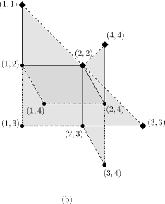
Figure 1: (a) The star graph $\Gamma$, (b) the two-particle configuration space $C_{2}(\Gamma)$, (c) the two-particle discrete configuration space $\mathcal{D}^{2}(\Gamma)$.

3 Morse theory in the nutshell

In this section we briefly present both classical and discrete Morse theories. We focus on the similarities between them and illustrate the ideas by several simple examples.

3.1 Classical Morse theory

The concept of classical Morse theory is essentially very similar to its discrete counterpart. Since the former is better known we have found it beneficial to first discuss the classical version. A good reference is the monograph by Milnor [15]. Classical Morse theory is a useful tool to describe topological properties of compact manifolds. Having such a manifold $M$ we say that a smooth function $f:M\rightarrow\mathbb{R}$ is a Morse function if its Hessian matrix at every critical point is nondegenerate, i.e.,

$$df(x)=0\,\,\Rightarrow\,\,\mathrm{det}\left(\frac{\partial^{2}f}{\partial x_{i}\partial x_{j}}\right)(x)\neq 0.$$ (13)

It can be shown that if $M$ is compact then $f$ has a finite number of isolated critical points [15]. The classical Morse theory is based on the following two facts:

1. Let $M_{c}=\{x\in M\,:\,f(x)\leq c\}$ denote a sub level set of $f$. Then $M_{c}$ is homotopy equivalent to $M_{c^{\prime}}$ if there is no critical value between the interval $(c,c\prime)$.

2. The change in topology when $M_{c}$ goes through a critical value is determined by the index (i.e., the number of negative eigenvalues) of the Hessian matrix at the associated critical point.

The central point of classical Morse theory are the so-called Morse inequalities, which relate the Betti numbers $\beta_{k}=\mathrm{dim}H_{k}(M)$, i.e. the dimensions of k-homology groups [13], to the numbers $m_{k}$ of critical points of index $k$, i.e.,

$$\sum_{k}m_{k}t^{k}-\sum_{k}\beta_{k}t^{k}=(1+t)\sum_{k}q_{k}t^{k},$$ (14)

where $q_{k}\geq 0$ and $t$ is an arbitrary real number. In particular (14) implies that $\beta_{k}\leq m_{k}$. The function $f$ is called a perfect Morse function iff $\beta_{k}=m_{k}$ for every $k$. Since there is no general prescription it is typically hard to find a perfect Morse function for a given manifold $M$. In fact a perfect Morse function may even not exist [16]. However, even if $f$ is not perfect we can still encode the topological properties of $M$ in a quite small cell complex. Namely it follows from Morse theory that given a Morse function $f$, one can show that $M$ is homotopic to a cell complex with $m_{k}$ $k$-cells, and the gluing maps can be constructed in terms of the gradient paths of $f$. We will not discuss this as it is far more complicated than in the discrete case.

3.2 Discrete Morse function

In this section we discuss the concept of discrete Morse functions for cell complexes as introduced by Forman [11]. Let $\alpha^{(p)}\in X$ denote a $p$ - cell. A discrete Morse function on a regular cell complex $X$ is a function $f$ which assigns larger values to higher-dimensional cells with ‘local’ exceptions.

Definition 1

A function $f\,:\,X\rightarrow\mathbb{R}$ is a discrete Morse function iff for every $\alpha^{(p)}\in X$ we have

$$\#\{\beta^{(p+1)}\supset\alpha\,:\,f(\beta)\leq f(\alpha)\}\leq 1,$$ (15)

$$\#\{\beta^{(p-1)}\subset\alpha\,:\,f(\beta)\geq f(\alpha)\}\leq 1.$$ (16)

In other words, definition 1 states that for any $p$ - cell $\alpha^{(p)}$, there can be $\mathbf{at\,\,most}$ one $(p+1)$ - cell $\beta^{(p+1)}$ containing $\alpha^{(p)}$ for which $f(\beta^{(p+1)})$ is less than or equal to $f(\alpha^{(p)})$. Similarly, there can be $\mathbf{at\,\,most}$ one $(p-1)$ - cell $\beta^{(p-1)}$ contained in $\alpha^{(p)}$ for which $f(\beta^{(p-1)})$ is greater than or equal to $f(\alpha^{(p)})$. Examples of a Morse function and a non-Morse function are shown in figure 3. The most important part of discrete Morse theory is the definition of a critical cell:

Definition 2

A cell $\alpha^{(p)}$ is critical iff

$$\#\{\beta^{(p+1)}\supset\alpha\,:\,f(\beta)\leq f(\alpha)\}=0,\,\,\mathrm{and}$$ (17)

$$\#\{\beta^{(p-1)}\subset\alpha\,:\,f(\beta)\geq f(\alpha)\}=0.$$ (18)

That is, $\alpha$ is critical if $f(\alpha)$ is greater than the value of $f$ on all of the faces of $\alpha$, and $f(\alpha)$ is greater than the value of $f$ on all cells containing $\alpha$ as a face. From definitions 1 and 2, we get that a cell $\alpha$ is noncritical iff either

1. $\exists\ {\rm unique}\ \tau^{(p+1)}\supset\alpha\,\,\,\,\,\ {\rm with}\ f(\tau)\leq f(\alpha),$ or

2. $\exists\ {\rm unique}\ \beta^{(p-1)}\subset\alpha\,\,\,\,\,\ {\rm with}\ f(\beta)\geq f(\alpha).$

It is quite important to understand that these two conditions cannot be simultaneously fulfilled, as we now explain. Let us assume on the contrary that both conditions (i) and (ii) hold. We have the following sequence of cells:

$$\tau^{(p+1)}\supset\alpha^{(p)}\supset\beta^{(p-1)}.$$ (19)

Since $\alpha^{(p)}$ is regular there is necessarily an $\tilde{\alpha}^{(p)}$ such that $\tau^{(p+1)}\supset\tilde{\alpha}^{(p)}\supset\beta^{(p-1)}$ (see figures 2(a),(b) for an intuitive explanation). Since $f(\tau)\leq f(\alpha)$, by definition 1 we have

$$f(\tilde{\alpha})<f(\tau).$$ (20)

We also know that $f(\beta)\geq f(\alpha)$ which, once again by definition 1, implies $f(\beta)<f(\tilde{\alpha})$. Summing up we get

$$f(\alpha)\leq f(\beta)<f(\tilde{\alpha})<f(\tau)\leq f(\alpha),$$ (21)

which is a contradiction.

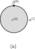
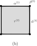
Figure 2: Examples of (a) an irregular cell complex. $\alpha^{(1)}$ is an irregular 1 - cell and $\beta^{(0)}$ is an irregular face of $\alpha^{(1)}$. (b) A regular cell complex with $\tau^{(2)}\supset\alpha^{(1)}\supset\beta^{(0)}.$

Following the path of classical Morse theory we define next the level sub-complex $K(c)$ by

$$K(c)=\cup_{f(\alpha)\leq c}\cup_{\beta\subseteq\alpha}\beta.$$ (22)

That is, $K(c)$ is the sub-complex containing all cells on which $f$ is less or equal to $c$, $\mathbf{{together\,\,with\,\,their\,\,faces}}$. Notice that by definition (1) a Morse function does not have to be a bijection. However, we have the following [11]:

Lemma 1

For any Morse function $f_{1}$, there exist another Morse function $f_{2}$ which is 1-1 and which has the same critical cells as $f_{1}$.

The process of attaching cells is accompanied by two important lemmas which describe the change in homotopy type of level sub-complexes when critical or noncritical cells are attached. Since, from lemma 1, we can assume that a given Morse function is 1-1, we can always choose the intervals $[a,b]$ below so that $f^{-1}([a,b])$ contains exactly one cell.

Lemma 2

[11] If there are no critical cells $\alpha$ with $f(\alpha)\in[a,b]$, then $K(b)$ is homotopy equivalent to $K(a)$.

Lemma 3

[11] If there is a single critical cell $\alpha^{(p)}$ with $f(\alpha)\in[a,b]$, then $K(b)$ is homotopy equivalent to

$$K(b)=K(a)\cup\alpha$$ (23)

and $\partial\alpha\subset K(a)$.

The above two lemmas lead to the following conclusion:

Theorem 3

[11] Let $X$ be a cell complex and $f\,:\,X\rightarrow\mathbb{R}$ be a Morse function. Then $X$ is homotopy equivalent to a cell complex with exactly one cell of dimension $p$ for each critical cell $\alpha^{(p)}$

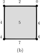
Figure 3: Examples of (a) a Morse function, and (b) a non-Morse function, since the 2-cell has value $5$ and there are two $1$-cells in its boundary with higher values assigned ($6$, $7$).

3.3 Discrete Morse vector field

From theorem 3 it follows that a given cell complex is homotopy equivalent to a cell complex containing only its critical cells, the so-called Morse complex. The construction of the Morse complex, in particular its boundary map (as well as the proof of theorem 3), depends crucially on the concept of a discrete vector field, which we define next. We know from definition 1 that the noncritical cells can be paired. If a $p$-cell is noncritical, then it is paired with either the unique noncritical $(p+1)$-cell on which $f$ takes an equal or smaller value, or the unique noncritical $(p-1)$-cell on which $f$ takes an equal or larger value. In order to indicate this pairing we draw an arrow from the $(p-1)$-cell to the $p$-cell in the first case or from the $p$-cell to the $(p+1)$-cell in the second case (see figure 4). Repeating this for all cells we get the so-called discrete gradient vector field of the Morse function. It also follows from section 3.2 that for every cell $\alpha$ exactly one of the following is true:

1. $\alpha$ is the tail of one arrow,

2. $\alpha$ is the head of one arrow,

3. $\alpha$ is neither the tail nor the head of an arrow.

Of course $\alpha$ is critical iff it is neither the tail nor the head of an arrow. Assume now that we are given a collection of arrows on some cell complex satisfying the above three conditions. The question we would like to address is whether it is a gradient vector field of some Morse function. In order to answer this question we need to be more precise. We define

Definition 3

A discrete vector field $V$ on a cell complex $X$ is a collection of pairs $\{\alpha^{(p)}\subset\beta^{(p+1)}\}$ of cells such that each cell is in at most one pair of $V$.

Having a vector field it is natural to consider its ‘integral lines’. We define the $V$ - path as a sequence of cells

$$\alpha_{0}^{(p)},\,\beta_{0}^{(p+1)},\,\alpha_{1}^{(p)},\,\beta_{1}^{(p+1)},\,\ldots,\alpha_{k}^{(p)},\,\beta_{k}^{(p+1)}$$ (24)

such that$\{\alpha_{i}^{(p)}\subset\beta_{i}^{(p+1)}\}\in V$ and $\beta_{i}^{(p+1)}\supset\alpha_{i+1}^{(p)}$. Assume now that $V$ is a gradient vector field of a discrete Morse function $f$ and consider a $V$ - path (24). Then of course we have

$$f(\alpha_{0}^{(p)})\geq f(\beta_{0}^{(p+1)})>f(\alpha_{1}^{(p)})\geq f(\beta_{1}^{(p+1)})>\ldots>f(\alpha_{1}^{(p)})\geq f(\beta_{k}^{(p+1)}).$$ (25)

This implies that if $V$ is a gradient vector field of the Morse function then $f$ decreases along any $V$-path which in particular means that there are no closed $V$-paths. It happens that the converse is also true, namely a discrete vector field $V$ is a gradient vector field of some Morse function iff there are no closed $V$ - paths [11].

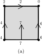
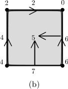
Figure 4: Examples of (a) a correct and (b) an incorrect discrete gradient vector fields; the 2-cell is the head of two arrows and the 1-cell is the head and tail of one arrow.

3.4 The Morse complex

Up to now we have learned how to reduce the number of cells of the original cell complex to the critical ones. However, it is still not clear how these cells are ‘glued’ together, i.e. what is the boundary map between the critical cells? The following result relates the concept of critical cells with discrete gradient vector fields [11].

Theorem 4

Assume that orientation has been chosen for each cell in the cell complex $X$. Then for any critical $(p+1)$-cell $\beta$ we have

$$\tilde{\partial}\beta=\sum_{critical\,\alpha^{(p)}}c_{\beta,\alpha}\alpha,$$ (26)

where $\tilde{\partial}$ is the boundary map in the cell complex consisting of the critical cells, whose existence is guaranteed by theorem 3, and

$$c_{\beta,\alpha}=\sum_{\gamma\in P(\beta,\alpha)}m(\gamma),$$ (27)

where $P(\beta,\alpha)$ is the set of all $V$ - paths from the boundary of $\beta$ to cells whose boundary contains $\alpha$ and $m(\gamma)=\pm 1$, depending on whether the orientation induced from $\beta$ to $\alpha$ through $\gamma$ agrees with the one chosen for $\alpha$.

The collection of critical cells together with the boundary map $\tilde{\partial}$ is called the Morse complex of the function $f$ and we will denote it by $M(f)$. Examples of the computation of boundary maps for Morse complexes will be given in section 5.

4 A perfect Morse function on $\Gamma$ and its discrete vector field.

In this section we present a construction of a perfect discrete Morse function on a $1$ - particle graph. It is defined analogously as in the classical case, i.e. the number of critical cells in each dimension is equal to the corresponding dimension of the homology group. The existence of such a function will be used in section 5 to construct a ‘good’ but not necessarily perfect Morse function on a $2$-particle graph.

Let $\Gamma=(V\,,\,E)$ be a graph with $v=|V|$ vertices and $e=|E|$ edges. In the following we assume that $\Gamma$ is connected and simple. Let $T$ be the spanning tree of $\Gamma$, i.e. $T$ is a connected spanning subgraph of $\Gamma$ such that $V(T)=V(\Gamma)$ and for any pair of vertices $v_{i}\neq v_{j}$ there is exactly one path in $T$ joining $v_{i}$ with $v_{j}$. We naturally have $|E(\Gamma)|-|E(T)|\geq 0$. The Euler characteristic of $\Gamma$ treated as a cell complex is given by

$$\chi(\Gamma)=v-e=\mathrm{dim}H_{0}(\Gamma)-\mathrm{dim}H_{1}(\Gamma)=b_{0}-b_{1}.$$ (28)

Since $\Gamma$ is connected, $H_{0}(\Gamma)=\mathbb{Z}$. Hence we get

$$b_{0}=1,$$ (29)

$$b_{1}=e-v+1.$$ (30)

On the other hand it is well known that $b_{1}=|E(\Gamma)|-|E(T)|$. Summing up from the topological point of view $\Gamma$ is homotopy equivalent to a wedge sum of $b_{1}$ circles. Our goal is to construct a perfect Morse function $f_{1}$ on $\Gamma$, i.e. the one with exactly $b_{1}$ critical $1$ - cells and one critical $0$ - cell. To this end we choose a vertex $v_{1}$ of valency one in $T$ (it always exists) and travel through the tree anticlockwise from it labeling vertices by $v_{k}$. The value of $f$ on the vertex $v_{k}$ is $f_{1}(k)=2k-2$ and the value of $f_{1}$ on the edge $(i,j)\in T$ is $f_{1}((i,j))=\mathrm{max}\left(f_{1}(i),\,f_{1}(j)\right)$. The last step is to define $f_{1}$ on the deleted edges $(i,j)\in E(\Gamma)\setminus E(T)$. We choose $f_{1}((i,j))=\mathrm{max}(f_{1}(i),\,f_{1}(j))+2$, where $v_{i},v_{j}$ are the boundary vertices of $(i,j)$. This way we obtain that all vertices besides $v_{1}$ and all edges of $T$ are not critical cells of $f_{1}$. The critical $1$ - cells are exactly the deleted edges. The following example clarifies this idea (see figure 5).

Example 2

Consider the graph $\Gamma$ shown in figure 5(a). Its spanning tree is denoted by solid lines and the deleted edges by dashed lines. For each vertex and edge the corresponding value of a perfect discrete Morse function $f_{1}$ is explicitly written. Notice that according to definition 2 we have exactly one critical $0$ - cell (denoted by a square) and four critical $1$ - cells which are deleted edges. The discrete vector field for $f_{1}$ is represented by arrows. The contraction of $\Gamma$ along this field yields the contraction of $T$ to a single point and hence the Morse complex $M(f_{1})$ is the wedge sum of four circles (see figure 5(b))

Figure 5: (a) The perfect discrete Morse function $f_{1}$ on the graph $\Gamma$ and its discrete gradient vector field. (b) The Morse complex $M(f_{1})$.

5 The main examples

In this section we present a method of construction of a ‘good’ Morse function on the two particle configuration space $\mathcal{D}^{2}(\Gamma_{i})$ for two different graphs $\Gamma_{i}$ shown in figures 6(a) and 8(a). We also demonstrate how to use the tools described in section 3 in order to derive a Morse complex and compute the first homology group. We begin with a graph $\Gamma_{1}$ which we will refer to as lasso (see figure 6(a)). The spanning tree of $\Gamma_{1}$ is denoted in black in figure 6(a). In figure 6(b) we see an example of the perfect Morse function $f_{1}$ on $\Gamma_{1}$ together with its gradient vector field. They were constructed according to the procedure explained in section 4. The Morse complex of $\Gamma_{1}$ consists of one $0$-cell (the vertex $1$) and one $1$-cell (the edge $(3,4)$).

Figure 6: (a) One particle on lasso, (b) The perfect discrete Morse function $f_{1}$

The two particle configuration space $\mathcal{D}^{2}(\Gamma_{1})$ is shown in figure 7(a). Notice that $\mathcal{D}^{2}(\Gamma_{1})$ consists of one $2$ - cell $(3,4)\times(1,2)$, six $0$ - cells and eight $1$ - cells. In order to define the Morse function $f_{2}$ on $\mathcal{D}^{2}(\Gamma_{1})$ we need to specify its value for each of these cells. We begin with a trial function $\tilde{f}_{2}$ which is completely determined once we know the perfect Morse function on $\Gamma_{1}$. To this end we treat $f_{1}$ as a kind of ‘potential energy’ of one particle. The function $\tilde{f}_{2}$ is simply the sum of the energies of both particles, i.e. the value of $\tilde{f}_{2}$ on a cell corresponding to a particular position of two particles on $\Gamma_{1}$ is the sum of the values of $f_{1}$ corresponding to this position. To be more precise we have for

$$\mathrm{0-cells:\,\,\,\,\,\,\,\,\,\,\,\,\,}\,\,\,\,\,\,\,\,\,\,\,\,\tilde{f}_{2}(i\times j) = f_{1}(i)+f_{1}(j),$$

$$\mathrm{1-cells:}\,\,\,\,\,\,\,\,\,\,\,\,\tilde{f}_{2}\left(i\times(j,k)\right) = f_{1}(i)+f_{1}\left((j,k)\right),$$

$$\mathrm{2-cells:}\,\,\,\tilde{f}_{2}\left((i,j)\times(k,l)\right) = f_{1}\left((i,j)\right)+f_{1}\left((k,l)\right).$$ (31)

In figure 7(b) we can see $\mathcal{D}^{2}(\Gamma_{1})$ together with $\tilde{f}_{2}$. Observe that $\tilde{f}_{2}$ is not a Morse function since the value of $\tilde{f}_{2}\left((3,4)\right)$ is the same as the value of $\tilde{f}_{2}$ on edges $4\times(2,3)$ and $3\times(2,4)$ which are adjacent to the vertex $(3,4)$. The rule that $0$ - cell can be the face of at most one $1$ - cell with smaller or equal value of $\tilde{f}_{2}$ is violated. In order to have Morse function $f_{2}$ on $\mathcal{D}^{2}(\Gamma_{1})$ we introduce one modification, namely

$$f_{2}\left(3\times(2,4)\right)=\tilde{f}_{2}\left(3\times(2,4)\right)+1,$$ (32)

and $f_{2}$ is $\tilde{f_{2}}$ on the other cells.

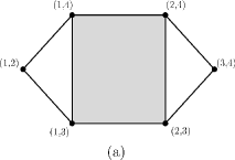
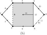
Figure 7: (a) The two particles on lasso, $\mathcal{D}^{2}(\Gamma_{1})$, (b) the discrete Morse function and its gradient vector field (c) the Morse complex (d) the topological gauge potential $\Omega$

Notice that the choice we made is not unique. We could have changed $\tilde{f}_{2}\left(4\times(2,3)\right)$ in a similar way and leave $\tilde{f}_{2}\left(3\times(2,4)\right)$ untouched. After the modification (32) we construct the corresponding discrete vector field for $f_{2}$. The Morse complex of $f_{2}$ consists of one critical $0$-cell (vertex $(1,2)$) and two critical $1$ - cells (edges $3\times(2,4)$ and $1\times(3,4)$). Observe that there are two different mechanisms responsible for criticality of these $1$ - cells. The cell $1\times(3,4)$ is critical due to the definition of trial Morse function $\tilde{f}_{2}$ and $3\times(2,4)$ has been chosen to be critical in order to make $\tilde{f}_{2}$ the well defined Morse function $f_{2}$. We will see later that these are in fact the only two ways giving rise to the critical cells. Notice finally that function $f_{2}$ is in fact a perfect Morse function and the Morse inequalities for it are equalities.

We will now consider a more difficult example. The one particle configuration space, i.e. graph $\Gamma_{2}$ together with the perfect Morse function and its gradient vector field are shown in figure 8(a) and 8(b).

Figure 8: (a) One particle on bow-tie (b) Perfect discrete Morse function

The construction of two particle configuration space is a bit more elaborate than in the lasso case and the result is shown in figure 9(a). Using rules given in (31) we obtain the trial Morse function $\tilde{f}_{2}$ which is shown in figure 9(b). The critical cells of $\tilde{f}_{2}$ and the cells causing $\tilde{f}_{2}$ to not be a Morse function are given in table 1.

Table 1: The critical cells of $\tilde{f}_{2}$ and the vertices and edges causing $\tilde{f}_{2}$ to not be a Morse function.

• Critical cells of the trial Morse fuction $\tilde{f}_{2}$
  0 - cells	$1\times 2$
  1 - cells	$1\times(4,5)$, $2\times(1,3)$
  2 - cells	$(1,3)\times(4,5)$

  $\tilde{f}_{2}$ is not Morse function because
  vertex	edges	value
  $(3,4)$	$3\times(2,4)$, $4\times(2,3)$	$\tilde{f}_{2}=10$
  $(3,5)$	$5\times(2,3)$, $3\times(2,5)$	$\tilde{f}_{2}=12$
  $(4,5)$	$5\times(2,4)$, $4\times(2,5)$	$\tilde{f}_{2}=14$

In figure 9(b) we have chosen $1$ - cells: $3\times(2,4)$, $3\times(2,5)$ and $4\times(2,5)$ to be critical, although we should emphasize that it is one choice out of eight possible ones. We will now determine the first homology group of the Morse complex $M(f_{2})$ and hence $H_{1}(\mathcal{D}^{2}(\Gamma_{2}))$. The Morse complex $M(f_{2})$ is the sum of $M_{0}(f_{2})$ consisting of one $0$-cell (vertex $1\times 2$), $M_{1}(f_{2})$ which consists of five critical $1$-cells and $M_{2}(f_{2})$ which is one critical $2$-cell $c_{2}=(1,3)\times(4,5)$.

The first homology is given by

$$H_{1}(M(f_{2}))=H_{1}(\mathcal{D}^{2}(\Gamma_{2}))=\frac{\mbox{Ker}\tilde{\partial}_{1}}{\mbox{Im}\tilde{\partial}_{2}}.$$ (33)

It is easy to see that $\tilde{\partial}_{1}c_{1}=0$ for any $c_{1}\in M_{1}(f_{2})$ and hence $\mbox{Ker}\tilde{\partial}_{1}=\mathbb{Z}^{5}$. What is left is to find $\tilde{\partial}c_{2}$ which is a linear combination of critical $1$-cells from $M_{1}(f_{2})$. According to formula (26) we take the boundary of $c_{2}$ in $C_{2}(\Gamma_{2})$ and consider all paths starting from it and ending at the $2$-cells containing critical $1$-cells (see table 2).

Table 2: The boundary of $c_{2}$.

• boundary of $c_{2}$	path	critical $1$ - cells	orientation
  $1\times(4,5)$	$\emptyset$	$1\times(4,5)$	+
  $5\times(1,3)$	$5\times(1,3)$, $(2,5)\times(1,3)$, $2\times(1,3)$. $5\times(1,3)$, $(2,5)\times(1,3)$, $3\times(2,5)$.	$2\times(1,3)$ $3\times(2,5)$	- -
  $3\times(4,5)$	$3\times(4,5)$, $(4,5)\times(2,3)$, $2\times(4,5)$, $(1,2)\times(4,5)$, $1\times(4,5)$.	$1\times(4,5)$	-
  $4\times(1,3)$	$4\times(1,3)$, $(1,3)\times(2,4)$, $2\times(1,3)$. $4\times(1,3)$, $(1,3)\times(2,4)$, $3\times(2,4)$.	$2\times(1,3)$ $3\times(2,4)$	+ +

Eventually taking into account orientation we get

$$\tilde{\partial}_{2}(c_{2})=1\times(4,5)-3\times(2,5)-2\times(1,3)-1\times(4,5)+$$ (34)

$$+3\times(2,4)+2\times(1,3)=-3\times(2,5)+3\times(2,4).$$ (35)

Hence,

$$H_{1}(\mathcal{D}^{2}(\Gamma_{2}))=\frac{\mbox{Ker}\tilde{\partial}_{1}}{\mbox{Im}\tilde{\partial}_{2}}=\mathbb{Z}^{4}.$$ (36)

The Morse complex $M(f_{2})$ is shown explicitly in figure 9(c). It is worth mentioning that in this example $f_{2}$ is not a perfect Morse function.

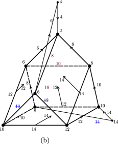
Figure 9: (a) Two particles on bow-tie (b) the discrete Morse function and its gradient vector field, (c) the Morse complex $M(f_{2})$.

6 Discrete Morse theory and topological gauge potentials

In this section we describe more specifically how the techniques of discrete Morse theory apply to the problem of quantum statistics on graphs. A more general discussion of the model can be found in [5]. Here we describe a particular representative example, highlighting the usefulness of discrete Morse theory.

Let $\Gamma$ be a graph shown in figure 7(a). The Hilbert space associated to $\Gamma$ is $\mathcal{H}=\mathbb{C}^{4}$ and is spanned by vertices of $\Gamma$. The dynamics is given by Schrödinger equation where the Hamiltonian $H$ is a hermitian matrix, such that $H_{jk}=0$ if $j$ is not adjacent to $k$ in $\Gamma$. As discussed in [5] this corresponds to the so-called tight binding model of one-particle dynamics on $\Gamma$. One can add to the model an additional ingredient, namely whenever particle hops between adjacent vertices of $\Gamma$ the wave function gains an additional phase factor. This can be incorporated to the Hamiltonian by introducing the gauge potential. It is an antisymmetric real matrix $\Omega$ such that each $\Omega_{jk}\in[0,\,2\pi[$ and $\Omega_{jk}=0$ if $j$ is not adjacent to $k$ in $\Gamma$. The modified Hamiltonian is then $H_{jk}^{\Omega}=H_{jk}e^{i\Omega_{jk}}$. The flux of $\Omega$ through any cycle of $\Gamma$ is the sum of values of $\Omega$ on the directed edges of the cycle. It can be given a physical interpretation of the Aharonov-Bohm phase.

In order to describe in a similar manner the dynamics of two indistinguishable particles on $\Gamma$ we follow the procedure given in [5]. The structure of the Hilbert space and the corresponding tight binding Hamiltonian are encoded in $\mathcal{D}^{2}(\Gamma)$. Namely, we have $\mathcal{H}_{2}=\mathbb{C}^{6}$ and is spanned by the vertices of $\mathcal{D}^{2}(\Gamma)$. The Hamiltonian is given by a hermitian matrix, such that $H_{j,k\rightarrow l}=0$ if $k$ is not adjacent to $l$ in $\Gamma$. The notation $j,k\rightarrow l$ describes two vertices $(j,k)$ and $(j,l)$ connected by an edge in $\mathcal{D}^{2}(\Gamma)$. The additional assumption which we add in this case stems from the topological structure of $\mathcal{D}^{2}(\Gamma)$ and is reflected in the condition on the gauge potential. Namely, since the 2-cell $c_{2}=(1,2)\times(3,4)$ is contractible we require that the flux through its boundary vanishes, i.e.

$$\Omega(\partial c_{2})=\Omega_{1,3\rightarrow 4}+\Omega_{4,1\rightarrow 2}+\Omega_{2,4\rightarrow 3}+\Omega_{3,2\rightarrow 1}=0\,\mathrm{mod}\,2\pi.$$ (37)

Our goal is to find the parametrization of all gauge potentials satisfying (37), up to the so-called trivial gauge, i.e. up to addition of $\Omega^{\prime}$ such that $\Omega^{\prime}(c)=0\,\mathrm{mod}\,2\pi$, for any cycle $c$. To this end we use discrete Morse theory. We first notice that the edges of $\mathcal{D}^{2}(\Gamma)$ which are heads of an arrow of the discrete Morse vector field form a tree. Without lose of generality we can put $\Omega_{j,k\rightarrow l}=0$ whenever $j\times(k,l)$ is a head of an arrow. Next, on the edges corresponding to the critical $1$-cells we put arbitrary phases $\Omega_{1,3\rightarrow 4}=\phi$ and $\Omega_{3,2\rightarrow 4}=\psi$. Notice that since $f_{2}$ is a perfect Morse function these phases are independent. The only remaining edge is $2\times(3,4)$ which is a tail of an arrow. In order to decide what phase should be put on it we follow the gradient path of the discrete Morse vector field which leads to edge $1\times(3,4)$. Hence $\Omega_{2,3\rightarrow 4}=\phi$. The effect of our construction is the topological gauge potential $\Omega$ which is given by two independent parameters (see figure 7(d)) and satisfies (37). The described reasoning can be mutatis mutandis applied to any graph $\Gamma$, albeit the phases on edges corresponding to the critical cells are not independent if $f_{2}$ is not a perfect Morse function. Finally notice, that in the considered example, the phase $\phi$ can be interpreted as an Aharonov-Bohm phase and $\psi$ as the exchange phase. The later gives rise to the anyon statistics.

7 General consideration for two particles

In this section we investigate the first Homology group $H_{1}(C_{2}(\Gamma))$ by means of discrete Morse theory. In section 5 the idea of a trial Morse function was introduced. Let us recall here that the trial Morse function is defined in two steps. The first one is to define a perfect Morse function on $\Gamma$. To this end one chooses the spanning tree $T$ in $\Gamma$. The vertices of $\Gamma$ are labeled by $1,\,2,\ldots,|V|$ according to the procedure described in section 4. The perfect Morse function $f_{1}$ on $\Gamma$ is then given by its value on the vertices and edges of $\Gamma$, i.e.

$$f_{1}(i)=2i-2,$$ (38)

$$f_{1}((j,k))=\mathrm{max}(f_{1}(j),\,f_{1}(k)),\,\,(j,k)\in T,$$ (39)

$$f_{1}((j,k))=\mathrm{max}(f_{1}(j),\,f_{1}(k))+2,\,\,(j,k)\in\Gamma\setminus T$$ (40)

When $f_{1}$ is specified the trial Morse function on $\mathcal{D}^{2}(\Gamma)$ is given by the formula

$$\mathrm{0-cells:\,\,\,\,\,\,\,\,\,\,\,\,\,}\,\,\,\,\,\,\,\,\,\,\,\,\tilde{f}_{2}(i\times j) = f_{1}(i)+f_{1}(j),$$

$$\mathrm{1-cells:}\,\,\,\,\,\,\,\,\,\,\,\,\tilde{f}_{2}\left(i\times(j,k)\right) = f_{1}(i)+f_{1}\left((j,k)\right),$$

$$\mathrm{2-cells:}\,\,\,\tilde{f}_{2}\left((i,j)\times(k,l)\right) = f_{1}\left((i,j)\right)+f_{1}\left((k,l)\right).$$ (41)

Let us emphasize that the trial Morse function is typically not a Morse function, i.e., the conditions of definition 1 might not be satisfied. Nevertheless, we will show that it is always possible to modify the function $\tilde{f}_{2}$ and obtain a Morse function $f_{2}$ out of it. In fact the function $\tilde{f_{2}}$ is not ’far’ from being a Morse function and, as we will see, the number of cells at which it needs fixing is relatively small. In the next paragraphs we localize the obstructions causing $\tilde{f}_{2}$ to not be a Morse function and explain how to overcome them.

The cell complex $\mathcal{D}^{2}(\Gamma)$ consists of $2$, $1$, and $0$-cells which we will denote by $\alpha$, $\beta$ and $\kappa$ respectively. For all these cells we have to verify the conditions of definition 1. Notice that checking these conditions for any cell involves looking at its higher and lower dimensional neighbours. In case of $2$-cell $\alpha$ we have only the former ones, i.e., the $1$-cells $\beta$ in the boundary of $\alpha$. For the $1$-cell $\beta$ both $2$-cells $\alpha$ and $0$-cells $\kappa$ are present. Finally for the $0$-cell $\kappa$ we have only $1$-cells $\beta$.

Our strategy is the following. We begin with the trial Morse function $\tilde{f}_{2}$ and go over all $2$-cells checking the conditions of definition 1. The outcome of this step is a new trial Morse function $\bar{f}_{2}$ which has no defects on $2$-cells. Next we consider all $1$-cells and verify the conditions of definition 1 for $\bar{f}_{2}$. It happens that they are satisfied. Finally we go over all $0$-cells. The result of this three-steps procedure is a well defined Morse function $f_{2}$. Below we present more detailed discussion. The proofs of all statements are in the Appendix.

1. Step 1 We start with a trial Morse function $\tilde{f}_{2}$. We notice first that for any edge $e\in T$ there is a unique vertex $v$ in its boundary such that $f_{1}(e)=f_{1}(v)$. In other words every vertex $v$, different from $v=1$, specifies exactly one edge $e\in T$ which we will denote by $e(v)$. Next we divide the set of $2$-cells into three disjoint classes. The first one contains $2$-cells $\alpha=e_{i}\times e_{j}$, where both $e_{i},e_{j}\notin T$. The second one contains $2$-cells $\alpha=e_{i}\times e(v)$, where $e(v)\in T$ and $e_{i}\notin T$, and the last one contains $2$-cells $\alpha=e(u)\times e(v)$, where both $e(u),e(v)\in T$. Now, since there are no $3$-cells, we have only to check that for each $2$-cell $\alpha$

   $$\#\{\beta\subset\alpha\,:\,\tilde{f}_{2}(\beta)\geq\tilde{f}_{2}(\alpha)\}\leq 1$$ (42)

   The following results are proved in the Appendix

   1. For the $2$-cells $\alpha=e_{i}\times e_{j}$ where both $e_{i},e_{j}\notin T$ the condition (42) is satisfied (see fact 1).

   2. For the $2$-cells $\alpha=e_{i}\times e(v)$ where $e_{i}\notin T$ and $e(v)\in T$ the condition (42) is satisfied (see fact 2).

   3. For the $2$-cells $\alpha=e(u)\times\rme(v)$ where both $e(u),e(v)\in T$ the condition (42) is not satisfied. There are exactly two $1$-cells $\beta_{1},\beta_{2}\subset\alpha$ such that $\tilde{f}_{2}(\beta_{1})=\tilde{f}_{2}(\alpha)=\tilde{f}_{2}(\beta_{2})$. They are of the form $\beta_{1}=u\times e(v)$ and $\beta_{2}=v\times e(u)$. The function $\tilde{f}_{2}$ can be fixed in two ways (see fact 3). We put $\bar{f}_{2}(\alpha)=\tilde{f}_{2}(\alpha)+1$ and either $\bar{f}_{2}(\beta_{1}):=\tilde{f}_{2}(\beta_{1})+1$ or $\bar{f}_{2}(\beta_{2}):=\tilde{f}_{2}(\beta_{2})+1$.

   The result of this step is a new trial Morse function $\bar{f}_{2}$, which satisfies (42).

2. Step 2 We divide the set of $1$-cells into two disjoint classes. The first one contains $1$-cells $\beta=v\times e$, where $e\notin T$ and the second one contains $\beta=v\times e(u)$, where $e(u)\in T$. For the $1$-cells within each of this classes we introduce additional division with respect to condition $e(v)\cap e=\emptyset$ (or $e(v)\cap e(u)=\emptyset$). Notice that all $1$-cells $\beta$ which were modified in Step 1 belong to the second class and satisfy $e(v)\cap e(u)=\emptyset$. Next we take a trial Morse function $\bar{f}_{2}$ and go over all $1$-cells $\beta$ checking for each of them if

   $$\#\{\alpha\supset\beta\,:\,\bar{f}_{2}(\alpha)\leq\bar{f}_{2}(\beta)\}\leq 1,$$ (43)

   $$\#\{\kappa\subset\beta\,:\,\bar{f}_{2}\geq\bar{f}_{2}(\beta)\}\leq 1.$$ (44)

   What we find out is

   1. For the $1$-cells $\beta=v\times e(u)$, where $e(u)\in T$ and $e(v)\cap e(u)\neq\emptyset$ the conditions (43, 44) are satisfied (see fact 4).

   2. For the $1$-cells $\beta=v\times e$, where $e\notin T$ and $e(v)\cap e\neq\emptyset$ the conditions (43, 44) are satisfied (see fact 5).

   3. For the $1$-cells $\beta=v\times e(u)$, where $e(u)\in T$ and $e(v)\cap e(u)=\emptyset$ the conditions (43, 44) are satisfied (see fact 6).

   4. For the $1$-cells $\beta=v\times e$, where $e\notin T$ and $e(v)\cap e=\emptyset$ the conditions (43, 44) are satisfied (see fact 7).

   Summing up the trial Morse function $\bar{f}_{2}$, obtained in Step 1 satisfies both (42) and (43), (44). We switch now to the analysis of $0$-cells.

3. Step 3 We divide the set of $0$-cells into four disjoint classes in the following way. We denote by $\tau(v)\neq v$ the vertex to which $e(v)$ is adjacent and call it the terminal vertex of $e(v)$. For any $0$-cell $\kappa=v\times u$ we have that either

   1. $e(v)\cap e(u)\neq\emptyset$ and the terminal vertex $\tau(v)$ of $e(v)$ is equal to $u$.

   2. $e(v)\cap e(u)\neq\emptyset$ and the terminal vertex $\tau(u)$ of $e(u)$ is equal to the terminal vertex $\tau(v)$ of $e(v)$.

   3. $e(v)\cap e(u)=\emptyset$.

   4. $\kappa=1\times u$.

   What is left is checking the following condition for any $0$-cell $\kappa$ :

   $$\#\{\beta\supset\kappa\,:\,\bar{f}_{2}(\beta)\leq\bar{f}_{2}(\kappa)\}\leq 1$$ (45)

   We find out that

   1. For the $0$-cell $\kappa=u\times v$ belonging to 3a the condition (45) is satisfied (see fact 8).

   2. For the $0$-cell $\kappa=u\times v$ belonging to 3b the condition (45) is not satisfied. There are exactly two $1$-cells $\beta_{1},\beta_{2}\supset\kappa$ such that $\bar{f}_{2}(\beta_{1})=\bar{f}_{2}(\kappa)=\bar{f}_{2}(\beta_{2})$. They are of the form $\beta_{1}=u\times e(v)$ and $\beta_{2}=v\times e(u)$. The function $\bar{f}_{2}$ can be fixed in two ways. We put $f_{2}(\beta_{1}):=\bar{f}_{2}(\beta_{1})+1$ or $f_{2}(\beta_{2}):=\bar{f}_{2}(\beta_{2})+1$ (see fact 9). Moreover, this change does not violate the Morse conditions at any $2$-cell containing $\beta_{i}$.

   3. For the $0$-cell $\kappa=u\times v$ belonging to 3c the condition (45) is satisfied (see fact 10)

   4. For the $0$-cell $\kappa=u\times v$ belonging to 3d the condition (45) is satisfied (see fact 11)

As a result of the above procedure we obtain the Morse function $f_{2}$. We can now ask the question which cells of $\mathcal{D}^{2}(\Gamma)$ are critical cells of $f_{2}$. Careful consideration of the arguments given in facts 1-11 lead to the following conclusions:

• The $0$-cell is critical if and only if it is $1\times 2$

• The $1$-cell is critical if and only if

  1. It is $v\times e$ where $e\notin T$ and $e(v)\cap e\neq\emptyset$ or $v=1$.

  2. Assume that $e(v)\cap e(u)\neq\emptyset$ and the terminal vertex $\tau(u)$ of $e(u)$ is equal to the terminal vertex $\tau(v)$ of $e(v)$. Then either the $1$-cell $v\times e(u)$ or the $1$-cell $u\times e(v)$ is critical, but not both.

• The $2$-cell is critical if and only if it is $e_{1}\times e_{2}$ where both $e_{i}\notin T$.

These rules are related to those given by Farley and Sabalka in [9]. As pointed out by an anonymous referee the freedom in choosing noncritical $1$-cells (described in fact 3) and critical $1$-cells (described in fact 9) is also present in Farley and Sabalka’s [8] construction.

8 Summary

We have presented a description of topological properties of two-particle graph configuration spaces in terms of discrete Morse theory. Our approach is through discrete Morse functions, which may be regarded as two-particle potential energies. We proceeded by introducing a trial Morse function on the full two-particle cell complex, $\mathcal{D}^{2}(\Gamma)$, which is simply the sum of single-particle potentials on the one-particle cell complex, $\Gamma$. We showed that the trial Morse function is close to being a true Morse function provided that the single-particle potential is a perfect Morse function on $\Gamma$. Moreover, we give an explicit prescription for removing local defects. The fixing process is unique modulo the freedom described in facts 3 and 9. The construction was demonstrated by two examples. A future goal would be to see if these constructions can provide any simplification in understanding of the results of [10].

9 Acknowledgments

I would like to thank Jon Keating and Jonathan Robbins for directing me towards the problem of quantum statistics on graphs and fruitful discussions. I am especially in debt to Jonathan Robbins for critical reading of the manuscript and many valuable comments. I would also like to thank the anonymous referees for their invaluable comments and suggestions which improved the final version of the paper. The support by University of Bristol Postgraduate Research Scholarship and Polish MNiSW grant no. N N202 085840 are gratefully acknowledged.

References

10 Appendix

In this section we give the proofs of the statements made in section 7. The following notation will be used. We denote by $D_{v}$ all edges of $\Gamma$ which are adjacent to $v$ and belong to $\Gamma-T$. Similarly by $T_{v}$ we denote all edges of $\Gamma$ which are adjacent to $v$ and belong to $T$, except one distinguished edge $e(v)\in T$, but not in $T_{v}$.

Fact 1

Let $\alpha=e_{1}\times e_{2}$ be a $2$-cell such that both $e_{1}$ and $e_{2}$ do not belong to $T$. The condition (42) is satisfied and $\alpha$ is a critical cell.

Proof. The two cell $e_{1}\times e_{2}$ is shown in the figure 10, where $e_{1}=(i,j)$ and $e_{2}=(k,l)$ and $i>j$, $k>l$. The result follows immediately from this figure.

Figure 10: The critical cell $e_{1}\times e_{2}$ where both $e_{1}$ and $e_{2}$ do not belong to $T$

Fact 2

Let $\alpha=e\times e(v)$ be a $2$-cell, where $e\notin T$ and $e(v)\in T$. Condition (42) is satisfied and $\alpha$ is a noncritical cell.

Proof. We of course assume that $e(v)\cap e=\emptyset$. The two cell $\alpha$ is shown on figure 11, where we denoted $e(v)=(v,\tau(v))$ and $e=(j,k)$. The result follows immediately from this figure.

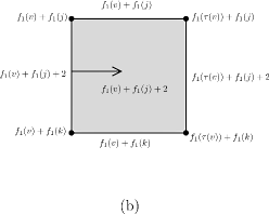
Figure 11: (a) $e(v)\cap e=\emptyset$ and $e\notin T$, (b) The noncritical cells $v\times e$ and $e(v)\times e$.

Fact 3

Let $\alpha=e(u)\times\rme(v)$ be the $2$-cells, where both $e(u),e(v)\in T$. Condition (42) is not satisfied. There are exactly two $1$-cells $\beta_{1},\beta_{2}\subset\alpha$ such that $\tilde{f}_{2}(\beta_{1})=\tilde{f}_{2}(\alpha)=\tilde{f}_{2}(\beta_{2})$. They are of the form $\beta_{1}=u\times e(v)$ and $\beta_{2}=v\times e(u)$. The function $\tilde{f}_{2}$ can be fixed in two ways. We put $\bar{f}_{2}(\alpha)=\tilde{f}_{2}(\alpha)+1$ and either $\bar{f}_{2}(\beta_{1}):=\tilde{f}_{2}(\beta_{1})+1$ or $\bar{f}_{2}(\beta_{2}):=\tilde{f}_{2}(\beta_{2})+1$.

Proof. The $2$-cell $e(v)\times e(u)$ when $e(v)\cap e(u)=\emptyset$ is presented in figure 12(a),(b). The trail Morse function $\tilde{f}_{2}$ requires fixing and two possibilities are shown on figure 12(c),(d). Notice that in both cases we get a pair of noncritical cells. Namely the $1$-cell $v\times e(u)$ and $2$-cell $e(v)\times e(u)$ for the situation presented in figure 12(c) and $1$-cell $u\times e(v)$, $2$-cell $e(v)\times e(u)$ for the situation presented in figure 12(d).

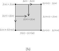
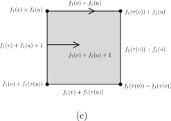
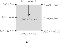
Figure 12: (a) Two edges of $T$ with $e(v)\cap e(u)=\emptyset$, (b) The problem of $2$-cell $e(v)\times e(u)$ (c),(d) two possible fixings of $\tilde{f}_{2}$

Fact 4

For the $1$-cells $\beta=v\times e(u)$, where $e(u)\in T$ and $e(v)\cap e(u)\neq\emptyset$ the conditions (43, 44) are satisfied.

Proof. Let us first calculate $\bar{f}_{2}(\beta)$. To this end we have to check if $\beta$ was modified in step 1. Notice that every $2$-cell which has $\beta$ in its boundary is one of the following forms:

1. $e(v)\times e(u)$

2. $e\times e(u)$ with $e\in D_{v}$

3. $e\times e(u)$ with $e\in T_{v}$

Case (1) is impossible since $e(v)\cap e(u)\neq\emptyset$. For any $2$-cell belonging to (2) the value of $\tilde{f}_{2}$ was not modified on the boundary of $e\times e(u)$ (see fact 2). Finally, for $2$-cells belonging to (3) the value of $\tilde{f}_{2}$ was modified on the boundary of $e\times e(u)$ but not on the cell $\beta$ (see fact 3). Hence $\bar{f}_{2}(v\times e(u))=\tilde{f}_{2}(v\times e(u))=f_{1}(v)+f_{1}(e(u))=f_{1}(v)+f_{1}(u)$. Let us now verify condition (44). The $1$-cell $\beta$ is adjacent to exactly two $0$-cells, namely $v\times u$ and $v\times\tau(u)$. We have $\bar{f}_{2}(v\times u)=\tilde{f}_{2}(v\times u)=f_{1}(v)+f_{1}(u)$ and $\bar{f}_{2}(v\times\tau(u))=\tilde{f}_{2}(v\times\tau(u))=f_{1}(v)+f_{1}(\tau(u))$. Now since $f_{1}(\tau(u))<f_{1}(u)$ condition (44) is satisfied. For condition (43) we have only to examine $2$-cells of forms (2) and (3) (listed above). For $2$-cells that belong to (2) we have $f_{2}(e\times e(u))=f_{1}(e)+f_{1}(e(u))>f_{1}(v)+f_{1}(u)+2$ and for $2$-cells that belong to (3) we have $f_{2}(e\times e(u))=f_{1}(e)+f_{1}(e(u))+1>f_{1}(v)+f_{1}(u)+1$. Hence in both cases $\bar{f}_{2}(e\times e(u))>\bar{f}_{2}(v\times e(u))$ and condition (43) is satisfied.

Fact 5

For the $1$-cells $\beta=v\times e$, where $e\notin T$ and $e(v)\cap e\neq\emptyset$ conditions (43, 44) are satisfied.

Proof. Let us first calculate $\bar{f}_{2}(\beta)$. To this end we have to check if $\beta$ was modified in step 1. Notice that every $2$-cell which has $\beta$ in its boundary is one of the following forms:

1. $e(v)\times e$

2. $e_{i}\times e$ with $e_{i}\in D_{v}$

3. $e_{i}\times e$ with $e_{i}\in T_{v}$

Case (1) is impossible since $e(v)\cap e\neq\emptyset$. For any $2$-cell belonging to (2) or (3) the value of $\tilde{f}_{2}$ was not modified on the boundary of $e_{i}\times e(u)$ (see fact 1 and 2). Hence $\bar{f}_{2}(v\times e)=\tilde{f}_{2}(v\times e)=f_{1}(v)+f_{1}(e)$. Let us now verify condition (44). To this end assume that $e=(j,k)$ with $j>k$. The $1$-cell $\beta$ is adjacent to exactly two $0$-cells, namely $v\times j$ and $v\times k$. We have $\bar{f}_{2}(v\times j)=\tilde{f}_{2}(v\times j)=f_{1}(v)+f_{1}(j)$ and $\bar{f}_{2}(v\times k)=\tilde{f}_{2}(v\times k)=f_{1}(v)+f_{1}(k)$. Now since $f_{1}(e)=\mathrm{max}(f_{1}(j),f_{1}(k))+2$ condition (44) is satisfied. For condition (43) we have only to examine $2$-cells of forms (2) and (3) (listed above). It is easy to see that in both cases $\bar{f}_{2}(e_{i}\times e)>\bar{f}_{2}(v\times e)$.

Fact 6

For the $1$-cells $\beta=v\times e(u)$, where $e(u)\in T$ and $e(v)\cap e(u)=\emptyset$ conditions (43, 44) are satisfied.

Proof. Let us first calculate $\bar{f}_{2}(\beta)$. To this end we have to check if $\beta$ was modified in step 1. Notice that every $2$-cell which has $\beta$ in its boundary is one of the following forms:

1. $e(v)\times e(u)$

2. $e\times e(u)$ with $e\in D_{v}$

3. $e\times e(u)$ with $e\in T_{v}$

For any $2$-cell belonging to (2) the value of $\tilde{f}_{2}$ was not modified on the boundary of $e\times e(u)$ (see fact 2). For the $2$-cells belonging to (3) the value of $\tilde{f}_{2}$ was modified on the boundary of $e\times e(u)$ but not on the cell $\beta$ (see fact 3). Finally for the $2$-cell $e(v)\times e(u)$ the value of $\tilde{f}_{2}$ was modified on the boundary of $e(v)\times e(u)$ and by fact 3 it might be the case that it was modified on $\beta$. Hence $\bar{f}_{2}(v\times e(u))=\tilde{f}_{2}(v\times e(u))=f_{1}(v)+f_{1}(e(u))=f_{1}(v)+f_{1}(u)$ or $\bar{f}_{2}(v\times e(u))=f_{1}(v)+f_{1}(u)+1$. Let us now verify condition (44). The $1$-cell $\beta$ is adjacent to exactly two $0$-cells, namely $v\times u$ and $v\times\tau(u)$. We have $\bar{f}_{2}(v\times u)=\tilde{f}_{2}(v\times u)=f_{1}(v)+f_{1}(u)$ and $\bar{f}_{2}(v\times\tau(u))=\tilde{f}_{2}(v\times\tau(u))=f_{1}(v)+f_{1}(\tau(u))$. Now since $f_{1}(\tau(u))<f_{1}(u)$ condition (44) is satisfied. For condition (43) we have to examine $2$-cells from (1), (2) and (3) (listed above). In case when $\bar{f}_{2}(v\times e(u))=f_{1}(v)+f_{1}(u)$ it is easy to see that $\bar{f}_{2}(e\times e(u))>\bar{f}_{2}(v\times e(u))$ for $e\in D_{v},T_{v}$ and $\bar{f}_{2}(e(v)\times e(u))>\bar{f}_{2}(v\times e(u))$. For $\bar{f}_{2}(v\times e(u))=f_{1}(v)+f_{1}(u)+1$ we still have $\bar{f}_{2}(e\times e(u))>\bar{f}_{2}(v\times e(u))$ for $e\in D_{v},T_{v}$ and $\bar{f}_{2}(e(v)\times e(u))=\bar{f}_{2}(v\times e(u))$. Hence condition (43) is satisfied in both cases.

Fact 7

For the $1$-cells $\beta=v\times e$, where $e\notin T$ and $e(v)\cap e=\emptyset$ conditions (43, 44) are satisfied.

Proof. Let us first calculate $\bar{f}_{2}(\beta)$. To this end we have to check if $\beta$ was modified in step 1. Notice that every $2$-cell which has $\beta$ in its boundary is one of the following forms:

1. $e(v)\times e$

2. $e_{i}\times e$ with $e_{i}\in D_{v}$

3. $e_{i}\times e$ with $e_{i}\in T_{v}$

For any $2$-cell belonging to (1), (2) and (3) the value of $\tilde{f}_{2}$ was not modified on the boundary of an appropriate $2$-cell (see fact 2 and 3). Hence $\bar{f}_{2}(v\times e)=\tilde{f}_{2}(v\times e)=f_{1}(v)+f_{1}(e)$. Let us now verify condition (44). To this end assume that $e=(j,k)$ with $j>k$. The $1$-cell $\beta$ is adjacent to exactly two $0$-cells, namely $v\times j$ and $v\times k$. We have $\bar{f}_{2}(v\times j)=\tilde{f}_{2}(v\times j)=f_{1}(v)+f_{1}(j)$ and $\bar{f}_{2}(v\times k)=\tilde{f}_{2}(v\times k)=f_{1}(v)+f_{1}(k)$. Now since $f_{1}(e)=\mathrm{max}(f_{1}(j),f_{1}(k))+2$ condition (44) is satisfied. For condition (43) we have to examine $2$-cells form (1), (2) and (3) (listed above). It is easy to see that $\bar{f}_{2}(e_{i}\times e)>\bar{f}_{2}(v\times e)$ for $e_{i}\in D_{v},\,T_{v}$ and $\bar{f}_{2}(e(v)\times e)=\bar{f}_{2}(v\times e)$.

Fact 8

For the $0$-cell $\kappa=u\times v$ such that $e(v)\cap e(u)\neq\emptyset$ with the terminal vertex $\tau(v)$ of $e(v)$ equal to $u$, condition (45) is satisfied.

Proof. The situation when $e(v)\cap e(u)\neq\emptyset$ and terminal vertex $\tau(v)$ of $e(v)$ is equal to $u$ is presented in the figure 13. For the $0$-cell $v\times u$ we have $\bar{f}_{2}=\tilde{f}_{2}(v\times u)=f_{1}(v)+f_{1}(u)$. Notice that there is exactly one edge $v\times e(u)$ for which $\bar{f}_{2}\left(v\times e(u))\right)=\bar{f}_{2}(v\times u)$. The function $\bar{f}_{2}$ on the other edges adjacent to $v\times u$ have a value greater than $\bar{f}_{2}(v\times u)$ and hence $v\times u$ and $v\times e(u)$ constitute a pair of noncritical cells.

Figure 13: $e(v)\cap e(u)\neq\emptyset$ and $\tau(v)=u$

Fact 9

For the $0$-cell $\kappa=u\times v$ such that $e(v)\cap e(u)\neq\emptyset$ with the terminal vertex $\tau(u)$ of $e(u)$ equal to the terminal vertex $\tau(v)$ of $e(v)$ condition (45) is not satisfied. There are exactly two $1$-cells $\beta_{1},\beta_{2}\supset\kappa$ such that $\bar{f}_{2}(\beta_{1})=\bar{f}_{2}(\kappa)=\bar{f}_{2}(\beta_{2})$. They are of the form $\beta_{1}=u\times e(v)$ and $\beta_{2}=v\times e(u)$. The function $\bar{f}_{2}$ can be fixed in two ways. We put $f_{2}(\beta_{1}):=\bar{f}_{2}(\beta_{1})+1$ or $f_{2}(\beta_{2}):=\bar{f}_{2}(\beta_{2})+1$.

Proof. The situation when $e(v)\cap e(u)\neq\emptyset$ and terminal vertex $\tau(u)$ of $e(u)$ is equal to terminal vertex $\tau(v)$ of $e(v)$ is presented in the figure 14(a),(b). For the $0$-cell $v\times u$ we have $\bar{f}_{2}(v\times u)=f_{1}(v)+f_{1}(u)$. There are two edges $v\times e(u)$ and $u\times e(v)$ such that $\bar{f}_{2}(v\times e(u))=\bar{f}_{2}(v\times u)=\bar{f}_{2}(u\times e(v))$. It is easy to see that the value of $\bar{f}_{2}$ on the other edges adjacent to $v\times u$ is greater than $\bar{f}_{2}(v\times u)$. So the function $\bar{f}_{2}$ does not satisfy condition (45) and there are two possibilities 14(c),(d) to fix this problem. Either we put $\bar{f}_{2}(v\times e(u))=\bar{f}_{2}(v\times u)+1$ or $\bar{f}_{2}(u\times e(v))=\bar{f}_{2}(v\times u)+1$. They both yield that the vertex $v\times u$ is non-critical. Notice finally that by the definitions of $f_{1}$ and $\tilde{f}_{2}$, increasing the value of $\bar{f}_{2}(\beta_{i})$ by one does not influence $2$-cells containing $\beta_{i}$ in their boundary.

Figure 14: (a) Two edges of $T$ with $e(v)\cap e(u)\neq\emptyset$, (b) The problem of $1$-cells $v\times(u,\tau(u))$ and $u\times(v,\tau(v))$ (c),(d) The two possible fixings of $\bar{f}_{2}$

Fact 10

For the $0$-cell $\kappa=u\times v$ such that $e(v)\cap e(u)=\emptyset$ condition (45) is satisfied.

Proof. This is a direct consequence of the modification made for the $2$-cell $\alpha=e(v)\times e(u)$ in step 1. Moreover, $\kappa$ is noncritical.

Fact 11

For the $0$-cell $\kappa=1\times u$ condition (45) is satisfied.

Proof. For the $0$-cell $1\times u$ we have $\bar{f}_{2}=\tilde{f}_{2}(v\times u)=f_{1}(u)$. Notice that there is exactly one edge $1\times e(u)$ for which $\bar{f}_{2}\left(1\times e(u)\right)=\bar{f}_{2}(1\times u)$. The function $\bar{f}_{2}$ on the other edges adjacent to $1\times u$ have a value greater than $\bar{f}_{2}(1\times u)$. Hence if $u\neq 2$ the $0$-cell $1\times u$ and the $1$-cell $1\times e(u)$ constitute a pair of noncritical cells. Otherwise $\kappa$ is a critical $0$-cell.

References

- [1] Souriau, J M 1970 Structure des syst mes dynamiques, Dunod, Paris.
- [2] Leinaas J M, Myrheim J 1977 On the theory of identical particles. Nuovo Cim.37B, 1–23.
- [3] Wilczek, F (ed.) 1990 Fractional statistics and anyon superconductivity. Singapore, Singapore: World Scientific.
- [4] Dowker, J S 1985 Remarks on non-standard statistics J. Phys. A: Math. Gen. 18 3521
- [5] Harrison J M, Keating J P and Robbins J M 2011 Quantum statistics on graphs Proc. R. Soc. A 8 January vol. 467 no. 2125 212-233
- [6] Balachandran A P, Ercolessi E 1992 Statistics on networks. Int. J. Mod. Phys. A 7, 4633 4654.
- [7] Abrams A 2000 Configuration spaces and braid groups of graphs. Ph.D. thesis, UC Berkley.
- [8] Prue P, Scrimshaw T 2009 Abrams’s stable equivalence for graph braid groups. arXiv:0909.5511
- [9] Farley D, Sabalka L 2005 Discrete Morse theory and graph braid groups Algebr. Geom. Topol. 5 1075-1109
- [10] Ko K H, Park H W 2011 Characteristics of graph braid groups. arXiv:1101.2648
- [11] Forman R 1998 Morse Theory for Cell Complexes Advances in Mathematics 134, 90145
- [12] Fox R H, Neuwirth L 1962 The braid groups, Math. Scand. 10, 119-126.
- [13] Hatcher A 2002 Algebraic Topology, Cambridge University Press
- [14] Ghrist R 2007 Configuration spaces, braids and robotics. Notes from the IMS Program on Braids, Singapore
- [15] Milnor J 1963 Classical Morse Theory, Princeton University Press
- [16] Ayala R, Fernandez-Ternero D, Vilches J A 2011 Perfect discrete Morse functions on 2-complexes. Pattern Recognition Letters, Available online 10.1016/j.patrec.2011.08.011.