HATSouth: a global network of fully automated identical wide-field telescopes

Abstract

HATSouth is the world’s first network of automated and homogeneous telescopes that is capable of year-round 24-hour monitoring of positions over an entire hemisphere of the sky. The primary scientific goal of the network is to discover and characterize a large number of transiting extrasolar planets, reaching out to long periods and down to small planetary radii. HATSouth achieves this by monitoring extended areas on the sky, deriving high precision light curves for a large number of stars, searching for the signature of planetary transits, and confirming planetary candidates with larger telescopes. HATSouth employs six telescope units spread over three prime locations with large longitude separation in the southern hemisphere (Las Campanas Observatory, Chile; HESS site, Namibia; Siding Spring Observatory, Australia). Each of the HATSouth units holds four 0.18 m diameter f/2.8 focal ratio telescope tubes on a common mount producing an $8.2\arcdeg\times 8.2\arcdeg$ field-of-view on the sky, imaged using four $\rm 4K\times\rm 4K$ CCD cameras and Sloan $r$ filters, to give a pixel scale of 3.7$\rm\arcsec pixel^{-1}$. The HATSouth network is capable of continuously monitoring 128 square arc-degrees at celestial positions moderately close to the anti-solar direction. We present the technical details of the network, summarize operations, and present detailed weather statistics for the three sites. Robust operations have meant that on average each of the six HATSouth units has conducted observations on $\sim 500$ nights over a two-year time period, yielding a total of more than 1 million science frames at four minute integration time, and observing $\sim 10.65$ hours per day on average. We describe the scheme of our data transfer and reduction from raw pixel images to trend-filtered light curves and transiting planet candidates. Photometric precision reaches $\sim 6$ mmag at 4 minute cadence for the brightest non-saturated stars at $r\approx 10.5$. We present detailed transit recovery simulations to determine the expected yield of transiting planets from HATSouth. We highlight the advantages of networked operations, namely, a threefold increase in the expected number of detected planets, as compared to all telescopes operating from the same site.

1. Introduction

Robotic telescopes first appeared about 40 years ago. The primary motivations for their development included cost efficiency, achieving consistently good data quality, and diverting valuable human time from monotonous operation into research. The first automated and computer-controlled telescope was the 0.2 m reflector of Washburn Observatory (McNall et al., 1968). Another noteworthy development was the Automated Photometric Telescope (APT; Boyd et al., 1984) project, which achieved a level of automation that enabled more than two decades of unmanned operations. As computer technology, microelectronics, software, programming languages, and interconnectivity (Internet) have developed, remotely-operated or fully-automated (often referred to as autonomous) telescopes have become widespread (see Castro-Tirado, 2010, for a review). A few prime examples are: the 0.75 m Katzman Automatic Imaging Telescope (KAIT; Filippenko et al., 2001) finding a large number of supernovae; the Robotic Optical Transient Search Experiment-I (ROTSE-I) instrument containing four 0.11 m diameter lenses, which for exampled detected the spectacular $V=8.9$ mag optical afterglow of a gamma ray burst at redshift of $z\approx 1$ (Akerlof et al., 1999); the LIncoln Near Earth Asteroid Research (LINEAR; Stokes et al., 1998) and Near Earth Asteroid Tracking (NEAT; Pravdo et al., 1999) projects using 1 m-class telescopes and discovering over a hundred thousand asteroids to date; the All Sky Automated Survey (ASAS; Pojmanski, 2002) employing a 0.1 m telescope to scan the entire sky and discover $\sim 50000$ new variables; the Palomar Transient Factory (PTF; Rau et al., 2009) exploring the optical transient sky, finding on average one transient every 20 minutes, and discovering $\sim 1500$ supernovae so far; the Super Wide Angle Search for Planets (SuperWASP; Pollacco et al., 2006) and Hungarian-made Automated Telescope Network (HATNet; Bakos et al., 2004) projects employing 0.1 m telescopes and altogether discovering $\gtrsim 100$ transiting extrasolar planets.

To improve the phase coverage of time-variable phenomena, networks of telescopes distributed in longitude were developed. We give a few examples below. One such early effort was the Smithsonian Astrophysical Observatory’s satellite tracker project (Whipple & Hynek, 1956; Henize, 1958), using almost identical hardware (Baker-Nunn cameras) at 12 stations around the globe, including Curaçao and Ethiopia. This network was manually operated. Another example is the Global Oscillation Network Group project (GONG; Harvey et al., 1988), providing Doppler oscillation measurements for the Sun, using 6 stations with excellent phase coverage for solar observations ($|\delta|\!<23.5\arcdeg$). The Whole Earth Telescope (WET; Nather et al., 1990) uses existing (but quite inhomogeneous) 1 m-class telescopes at multiple locations in organized campaigns to monitor variable phenomena (Provencal et al., 2012). The PLANET collaboration (Albrow et al., 1998) employed existing 1 m-class telescopes to establish a round-the-world network, leading to the discovery of several planets via microlensing anomalies. Similarly, RoboNet (Tsapras et al., 2009) used 2 m telescopes at Hawaii, Australia, and La Palma to run a fully automated network to detect planets via microlensing anomalies. ROTSE-III (Akerlof et al., 2003) has been operating an automated network of 0.5 m telescopes for the detection of optical transients, with stations in Australia, Namibia, Turkey and the USA.

The study of transiting extrasolar planets (TEPs) has greatly benefited from the development of automated telescopes and networks. Mayor et al. (2009) and Howard et al. (2010, 2011) concluded that $\sim 1.7\%$ of dwarf stars harbor planets with radii between $3R_{\earth}$ and $32R_{\earth}$ and periods less than $20$ d; such planets could be be detected by ground-based surveys such as ours. When coupled with the geometric probability that these planets transit their host stars as seen from the Earth, only $\sim 0.11\%$ of dwarf stars have TEPs with the above parameters. Further, in a brightness limited sample with e.g. $r\!<\!12$ mag, only $\sim 40\%$ of the stars are A5 to M5 dwarfs (enabling spectroscopic confirmation and planetary mass measurement), thus fewer than 1 in 2000 of the $r\!<\!12$ mag stars will have a moderately ($>3\,R_{\earth}$) large radius and short period ($P<20$ d) TEP. Consequently, monitoring of tens of thousands of stars at high duty cycle and homogeneously optimal data quality is required for achieving a reasonable TEP detection yield.

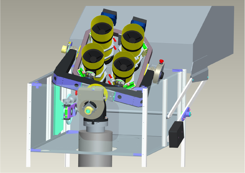
Figure 1.— Engineering model of the HS₄ unit, depicting the dome, telescope mount, optical tubes and CCDs. The asymmetric clamshell dome can open/close with the telescope in any position. The equatorial fork mount holds a large frame that supports the four astrographs and CCDs, tilted $\sim 4\arcdeg$ with respect to each other, and therefore capable of producing a mosaic image of $8\arcdeg\times 8\arcdeg$.

To date approximately 140 TEPs have been confirmed, characterized with RVs to measure the planetary mass, and published. These have been found primarily by photometric transit surveys employing automated telescopes (and networks in several cases) such as WASP (Pollacco et al., 2006), HATNet (Bakos et al., 2004), CoRoT (Baglin et al., 2006), OGLE (Udalski et al., 2002), Kepler (Borucki et al., 2010), XO (McCullough et al., 2005), and TrES (Alonso et al., 2004). In addition, Kepler has found over 2000 strong planetary candidates, which have been instrumental in determining the distribution of planetary radii. Many ($\sim 40$) of these planetary systems have been confirmed or “validated” (Batalha et al., 2012, and references therein), although not necessarily by radial velocity measurements. While the sample of $\sim 140$ fully confirmed planets with accurate mass measurements is large enough to reveal tantalizing correlations among various planetary (mass, radius, equilibrium temperature, etc.) and stellar (metallicity, age) properties, given the apparent diversity of planets, it is still insufficient to provide a deep understanding of planetary systems. For only the brightest systems is it currently possible to study extrasolar planetary atmospheres via emission or transmission spectroscopy; the faintest system for which a successful atmosphere study has been performed is WASP-12, which has $V\approx 11.6$ mag; (Madhusudhan et al., 2011). Similarly, it is only for the brightest systems that one can obtain a high S/N spectrum in an exposure time short enough to resolve the Rossiter-McLaughlin effect (Holt, 1893; Schlesinger, 1910; Rossiter, 1924; McLaughlin, 1924), and thereby measure the projected angle between the planetary orbital axis and the stellar spin axis.

The existing sample of ground-based detections of TEPs around bright stars is highly biased toward Jupiter-size planets with periods shorter than 5 days. Only 13 of the $\sim 140$ RV-confirmed TEPs have masses below $0.1\,M_{\rm J}$, and only 12 have periods longer than 10 days. The bias towards short periods is due not only to the higher geometric probability of short-period transits, and relative ease of their confirmation with spectroscopic (radial-velocity) observations, but also to the low duty cycle of single-longitude surveys. Although the transiting hot Jupiters provide an opportunity to study the properties of planets in an extreme environment, they are not representative of the vast majority of planetary-mass objects in the Universe, which are likely to be of lower mass, and on longer period orbits. While other planet-detection methods, such as microlensing, have proven to be efficient at discovering long-period and low-mass planets (Gould et al., 2010; Dong et al., 2009), these methods are primarily useful for studying the statistical distributions of periods and masses of planets, and cannot be used to study the other physical properties of individual planets, which can only be done for TEPs.

In this paper we descript HATSouth, a set of new ground-based telescopes which form a global and automated network with exactly identical hardware at each site, and with true 24-hour coverage all year around (for any celestial object in the southern hemisphere, and “away” from the Sun in a given season). HATSouth is the first such network, although many more are planned. The Las Cumbres Observatory Global Telescope (LCOGT; Brown et al., 2010), SOLARIS (Konacki et al., 2011), and the KMTNet (Kim et al., 2010) will all form global, homogeneous and automated networks when they are completed.

The HATSouth survey, in operation since late 2009, has the northern hemisphere HATNet survey (Bakos et al., 2004) as its heritage. HATSouth, however, has two important distinctions from HATNet, and from all other ground-based transit surveys. The first and most important is its complete longitudinal coverage. The network consists of six robotic instruments distributed across three sites on three continents in the southern hemisphere: Las Campanas Observatory (LCO) in Chile, the High Energy Stereoscopic System (HESS) site in Namibia, and Siding Springs Observatory (SSO) in Australia. The geographical coordinates of these sites are given in Tab. 1 below. The longitude distribution of these observatories enables round-the-clock monitoring of selected fields on the sky. This greatly increases the detectability of TEPs, particularly those with periods in excess of a few days. This gives HATSouth an order of magnitude higher sensitivity than HATNet to planets with periods longer than 10 days, and its sensitivity towards $P\approx 15-20$ d planets is better than HATNet’s sensitivity at $P\approx 8$ d . This is encouraging given that HATNet has demonstrated sensitivity in this regime with the discoveries of HAT-P-15b (Kovács et al., 2010) and HAT-P-17b (Howard et al., 2012) at $P>10$ d. Note that for mid- to late-M dwarf parent stars, planets with $\sim 15$ d periods lie in the habitable zone.

The second difference between HATSouth and HATNet is that each HATSouth astrograph has a larger aperture than a HATNet telephoto lens (0.18 m vs. 0.11 m), plus a slower focal ratio and lower sky background (per pixel, and under the point spread function of a star), which allows HATSouth to monitor fainter stars than HATNet. Compared to HATNet, this increases the overall number of dwarf stars observed at 1% photometry over a year by a factor of $\sim 3$; more specifically the number of K and M dwarf stars monitored effectively is increased by factors of 3.1 and 3.6, respectively (the numbers take into account the much larger surface density of dwarf stars and the somewhat smaller field-of-fiew of HATSouth, along with slight differences in the observing tactics). This increases the expected yield of small-size planets, and opens up the possibility of reaching to the super-Earth range. Furthermore, the ratio of dwarf stars to giant stars that are monitored at 1% photometric precision in the HATSouth sample at $|b|\approx 20\arcdeg$ is about twice that of HATNet, yielding a lower false alarm rate. Furthermore, despite greater stellar number densities, stellar crowding is less than with HATNet due to HATSouth’s three times finer spatial (linear) resolution. Note that while the stellar population monitored is generally fainter than that of HATNet, they are still within the reach of follow-up facilities.

The layout of the paper is as follows. In Section 2 we describe the HATSouth hardware in detail, including the telescope units (§ 2.1), weather sensing devices (§ 2.2), and the computer systems (§ 2.3). In Section 3 we detail the instrument control software. The HATSouth sites and operations are laid out in Section 4. We give details on the site specifics (§ 4.1), the scheme of nightly operations (§ 4.2), and present observing statistics for two years (§ 4.6). Data flow and analysis are described in Section 5, and the expected planet yield is calculated using detailed simulations in Section 6.

2. The HATSouth hardware

Each of the three HATSouth stations hosts two fully automated “observatories”, referred to as HS₄ units. One HS₄ unit holds 4 telescope tubes and 4 CCDs attached to a robotic mount, and enclosed by a robotic dome. The HS₄ units are controlled via computers from a dedicated control building that is $\sim 10$ meters north of the telescopes. The control building has multiple uses. It hosts a low-light web camera for monitoring telescopes (§ 2.2), all the computing equipment (§ 2.3), and all tools and spare components used for telescope maintenance and repair. The roof of the building is populated by weather sensing devices and an all-sky camera (§ 2.2). In the following subsections we describe the hardware components in more detail.

2.1. The HS₄ unit

An HS₄ unit is a fully automated observatory consisting of the following components:

• A Fornax F150 equatorial fork mount,

• Four 18 cm aperture f/2.8 Takahashi hyperbolic astrograph optical tube assemblies (OTAs),

• Four custom-built automated focuser units, each mounted to an OTA,

• Four Apogee U16m $\rm 4K\times\rm 4K$ CCD detectors, each mounted to a focuser unit,

• An asymmetric clamshell dome with weather sensing devices,

• A weatherproof electronic box attached to the dome, with power supplies, instrument control electronics and communication related electronics,

• An instrument control and data acquisition computer that is responsible for controlling all the above, and which is hosted in the nearby control building.

The four optical tubes are tilted with respect to each other to have a small overlap along the edges of the individual fields of view (FOV), and to produce a mosaic FOV spanning $8.2\arcdeg\times 8.2\arcdeg$ on $\rm 8K\times\rm 8K$ pixels altogether with a scale of $3.7\rm\arcsec pixel^{-1}$. Since two HS₄ instruments are located at each site, and they are pointed at different fields, one site monitors a 128$\Box^{\circ}$ sky area. Each of the three HATSouth sites have the same field setup, and because of the near-optimal longitude separation of the three sites, the HATSouth network is capable of continuously monitoring a 128$\Box^{\circ}$ sky area (in the anti-solar direction). In the following we present more information on the instrument parameters. These are also summarized in Tab. 1. The engineering design is shown in Fig. 1.

Figure 2.— Periodic errors (displacement in RA) of the HATSouth mount. The solid curve with solid circles shows the performance of the mount without tracking correction during a series of 30 s exposures. Periodic errors with $\sim 10\arcsec$ peak-to-peak amplitude are seen. The dashed curve with open circles shows the same experiment, repeated two days later, with the TDM tracking correction turned on. Long term drifts have been removed by a simple fit of a second order polynomial, yet some trends remain (no astrometry and subsequent corrections were applied in these tests). Using the TDM, the amplitude of the short term periodicity is reduced to $\sim 0.5\arcsec$ peak-to-peak amplitude where no drift is present. Overall, including longer term drifts, this translates to just $\sim 1.2\arcsec$ (median) displacement over 4 minute integrations.

2.1.1 The telescope mount

The Fornax F150 equatorial fork mount was designed, developed and constructed by our team specifically for the HATSouth project. Initial polar alignment of the mount is performed using a polar telescope that fits in the right ascension (RA) axis of the mount. The alignment is then refined by taking polar exposures and by adjusting the angle of the polar axis using fine alignment screws.

The RA axis is fitted with three inductive proximity sensors; one for the two end positions on the east and west, and the third one for the so-called home position very close to the meridian. Similarly, for the declination (DEC) axis we have proximity sensors for the polar and northern horizon end position, and one for the home position that roughly coincides with the celestial equator. When the mount reaches either the end or home positions the relevant proximity sensor is activated and alerts the electronics and the control software. If any of the end proximity sensors is activated during normal operation of the mount, telescope motion is inhibited by the software. If, for some reason, the proximity sensors fail, we have a second level of protection in the form of electronic limit switches just beyond the proximity sensor positions. If these are activated, then the motion of the telescope mount in that direction is inhibited directly by electronics, without relying on the control software. Finally, if the electronic limit switches fail, the mount hits the mechanical end positions, and any further motion is taken up by a clutch system on both the RA and DEC axes. We found that this level of redundancy in safety measures is essential for robust automated operation.

The exact position of the home sensors was measured during telescope installation via astrometry, and is re-calibrated every time a change in the hardware necessitates. The hour angle of the RA home position is determined to an accuracy of $\sim 25\arcsec$, and the declination of the DEC home position to $\sim 10\arcsec$. The mount has the capability to find and settle on the home position from any starting position within at most $\sim 200$ seconds, and more typically in 1 minute, using an iterative scheme and information from the proximity sensors. Following this homing procedure, which we perform at the beginning of each night, and using the local sidereal time (based on our GPS or the Network Time Protocol, see § 2.3), the pointing of the mount is known at an accuracy of $\lesssim 1\arcmin$.

The RA gear of the mount consists of a 292 mm diameter bronze cogwheel with 192 teeth. It is driven by a worm-drive, which, in turn, is driven by a two-phase stepper motor through sprockets and gears (with an additional 1:4.5 gear ratio). The resulting overall gear ratio is 1:864, so one full turn of the stepper motor axis corresponds to a 1/864 turn of the RA axis. The stepper motor receives the clock and direction signals from the printer port of the control computer through the control electronics. One microstep of the motor corresponds to 0.5″ resolution on the celestial equator (or 1/30 seconds of time in RA), i.e. the mount is driven at $\approx 30.08$ Hz during sidereal rate tracking. The mount has a massive fork with a span of 830 mm holding a rectangular frame on its DEC axis. This frame holds the four Takahashi optical tube assemblies (OTAs) through a mechanism that allows fine tilting of each optical tube in two perpendicular directions, so as to achieve a well aligned mosaic image. The main DEC axis gear consists of a 195 mm diameter cogwheel with 192 teeth. It is driven in a similar fashion to the RA gear, and one microstep on the motor corresponds to 0.5″. We set the maximal speed of the RA and DEC axes to be 2.2°/s (corresponding to 16 KHz drive frequency), and we typically ramp up in 50 steps over 3 degrees to the maximal speed during coarse motion. These parameters are fully adjustable from our control software.

Our pointing accuracy (median offset from the desired position) using this coarse motion is $\sim 140\arcsec$ (RA) and $\sim 55\arcsec$ (DEC) on the sky without a telescope pointing model, but after correcting for refraction. The accuracy is primarily limited by various flexures in the fork and the DEC frame, and by the imperfect polar alignment. This accuracy for coarse motion is adequate since it represents at most 0.5% of our $8\arcdeg\times 8\arcdeg$ FOV and we have the capability of doing astrometry on our images at sub-arcsecond accuracy, if these images contain at least a few hundred stars (typical numbers under normal conditions are $\mathcal{O}(10^{4})$). Following coarse motion pointing to a position, and initial astrometry, we then use fine motion to correct the position of the telescope with a small angle movement at low speed. To correct for a significant backlash we added an encoder to the DEC axis, and special electronics that together form a closed-loop control of the position when performing fine motion movements. We also have an encoder on the RA axis, which is used for precise sidereal rate tracking (see later). Fine motion in RA is performed by stopping or speeding up tracking. After a few exposures, we typically reach and maintain better than 10″ accuracy (in radial distance) while observing the same field.

Periodic tracking errors are inherently present in systems with worm-and-wheel gearing. It is common to have $\sim 10\arcsec$ positional variation in RA on the celestial equator. We carried out tracking tests to measure the periodic error of the Fornax F150 mounts. A selected field that culminates in zenith was observed for 2 hours at 30-second cadence from hour angle $-1$ hour to $+1$ hour. We found periodic errors with a peak-to-peak amplitude of $\lesssim 10\arcsec$ (median), and measured the main period to be $\sim 450$ seconds (Fig. 2). This matches the period expected from the engineering design. The tests were performed without using tracking correction (see below).

The movement of stars with respect to the CCD lattice leads to unwanted noise in the photometry, and the above tracking error would correspond to a large $\sim 5.6\arcsec$ (1.5 pixel) median displacement in RA during our typical 240 s integrations. One common solution for suppressing periodic errors is auto-guiding on stars by using separate optics (or a pick-off mirror) and a guide CCD. Autoguiding, however, is a sensitive procedure that requires acquiring suitable guide-stars, and it would lead to a large increase in hardware and operational complexity that we were keen to avoid. We thus used a hybrid solution, developed by our team. This is the “Telescope Drive Master” (TDM), consisting of an encoder on the RA axis, and a closed-loop control system that corrects the tracking clock signals based on the feedback from the encoder (see review by di Ciccio, 2011). Our tracking precision with the TDM is greatly improved, as exhibited in Fig. 2. The mean displacement during a 240 s integration is reduced by a factor of five, to $\sim 1.2\arcsec$ (0.3 pixel) on the celestial equator.

Table 1 System parameters for the HATSouth project.

Parameter	Value
Telescope Mount and Dome
Initial positioning accuracy (DEC)	$\sim 55\arcsec$
Initial positioning accuracy (RA)	$\sim 140\arcsec$
Periodic error (peak-to-peak, no TDM)	$\lesssim 10\arcsec$
Periodic error (with TDM)	$0.5\arcsec$
Tracking error in 4 minutes (with TDM)	$1.2\arcsec$
Coarse motion speed	2.2°/s
Stepper motor resolution	0.5″/step
Telescope home time (typical)	60 s
Telescope home time (max)	200 s
Dome opening/closing time	80 s
Optical Tube Assemblies
Clear aperture of primary mirror	180 mm
Secondary mirror (projected diameter)	80 mm
Focal ratio	2.8
Focal length	500 mm
Focusing accuracy	$2\,\mu m$
Filter	Sloan $r$
CCDs
Chip	Kodak KAF 16803
Number of pixels	$\rm 4K\times\rm 4K$
Pixel size	$9\,\mu m$
Full-well capacity	100,000$e^{-}$
Gain	1.4$\rm[e^{-}/ADU]$
Readout noise	7.7$e^{-}$
Cooling with respect to ambient	$\Delta T=45\,\rm^{\circ}C\;$
Dark current at $-30\rm^{\circ}C\;$	0.009$e^{-}$/s
Readout time	25 s
Combined Instrument Parameters
Pixel scale	3.7 $\rm\arcsec pixel^{-1}$
Field of view for single OTA	$4.18\times 4.18\arcdeg$
Mosaic field of view	$8.2\times 8.2\arcdeg$
Vignetting (edge/corner)	67%/46%
Zeropoint magnitude (1 ADU/s)	$r\approx 18.9$
5-$\sigma$ detection threshold	$r\approx 18.5$
Photometric precision at $r=11$ mag	0.006 mag/240 s
Photometric precision at $r=13.3$ mag	0.01 mag/240 s
Duty cycle	73%
Data flow
Raw compressed pixel data	19 TB/year
Calibrated pixel data and photometry	$\sim 60$ TB/year
Sites
Las Campanas Observatory, longitude	$70\arcdeg 42\arcmin 03.06\arcsec$ W
Latitude	$29\arcdeg 00\arcmin 38.65\arcsec$ S
Elevation	2285 m
Useful dark time	8.48 hr/night
HESS site, longitude	$16\arcdeg 30\arcmin 10.17\arcsec$ E
Latitude	$23\arcdeg 16\arcmin 23.32\arcsec$ S
Elevation	1800 m
Useful dark time	7.15 hr/night
Siding Spring Observatory, longitude	$149\arcdeg 03\arcmin 43.39\arcsec$ E
Latitude	$31\arcdeg 16\arcmin 20.47\arcsec$ S
Elevation	1165 m
Useful dark time	4.64 hr/night

Note. — For more explanation on the data in this table see the main text.

2.1.2 The optical tube assemblies

We use Takahashi $\epsilon$-$180$ ED astrographs as our optical tube assemblies (OTAs), which have a collecting area well matched to our project goal. They provide the fast focal ratio and high quality optics we require at an affordable price. Each HATSouth mount holds four such Takahashi astrographs. The $\epsilon$-$180$ astrograph is a catadioptric system with an f/3.66 hyperbolic primary mirror of 180 mm clear aperture, a flat diagonal secondary mirror of 80 mm diameter (as projected along the optical axis), and an extra low dispersion two-element Ross-corrector that flattens the field, reduces the focal ratio to f/2.8, and reduces coma and chromatism. The resulting focal length is 500 mm. The aluminum optical tube is compact, with a length of 568 mm, an outer diameter of 265 mm, and a total weight of 10.7 kg. The HATSouth mount was built to accommodate the combined weight of the four OTAs and CCDs ($\sim 70$ kg) on the DEC axis.

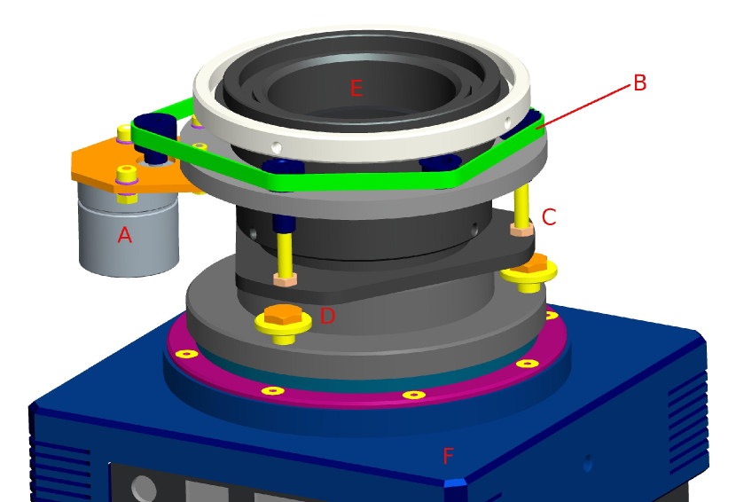
Figure 3.— Engineering model of the HS₄ focuser unit, replacing the original Takahashi focuser. Displacement is driven through an tooth timing belt mating with small cogwheels on three fine-threaded screws that ensure symmetric driving. Labeled are “A”: stepper motor, “B”: sprocket, “C”: fine-threaded drive, “D”: CCD tilt screws, “E”: Ross-corrector, “F”: CCD.

We removed the original Takahashi focusers from the OTAs, and replaced them with custom-built focuser units (Fig. 3) that allow for very fine electronic focus control via a two-phase stepper motor. For optimal image quality, the focal plane has to be fixed 77 mm away from the last vertex of the Ross-corrector lens (that is 56 mm from the Ross-corrector housing). This means that the corrector-lens, the filter, and the CCD form a single moving unit, which is moved perpendicular to the optical tube when focusing. One step of the focuser corresponds to a motion of $2\,\mu m$, and we make on the order of 1000 steps (2 mm) with the focusers during a typical night to compensate for temperature changes, tube flexure and other effects. The moving unit is tightly held by three bearings, minimizing off-axis wobble. The force from the two-phase stepper motor is transmitted through a tooth timing belt going around the entire focuser, and mating with small cogwheels on three fine-threaded screws that ensure symmetric driving (at 120° offset) of the moving unit. The entire focuser unit is enclosed in a custom-made velvet sleeve to prevent dust and other material getting onto drive mechanism or into the focus unit itself.

The light leaving the Ross corrector first goes through a 5 mm thick $50\times 50$ mm Sloan $r$ filter ($\sim 550$–700 nm) manufactured by Asahi Spectra. It then passes through the two camera windows of the CCD. Each window is made of 1.5 mm thick UV fused silica with a broad-band (400–700 nm) antireflectant (BBAR) coating.

As before, one prime consideration was to build a system that is virtually maintenance-free, or at least, where maintenance is made easy. The Newtonian design is prone to collecting dust and unwanted objects inside the tube, and is very laboursome to clean. For example, black mamba snakes (Dendroaspis polylepis), which are common in Namibia, are notoriously hard to remove from a telescope tube. Thus, we sealed the front of the OTA by installing a flat optical glass. We used Schott B270 glass with 5.5 mm thickness, 242 mm clear aperture, $<\!0.015$ mm wedge, and transmitted wavefront error smaller than one wavelength at 633 nm. The glass was coated for anti-reflection on both sides with $R\!<\!0.5\%$ at 570–710 nm. The optical glass was placed in a custom-built circular carrier, and can be removed easily for cleaning by attaching a fitted handle to the outer rim and then releasing three screws.

We also designed a dewcap that mounts on the front of the OTA, primarily to decrease scattered moonlight. The dewcap also contains a low power (4W) heating coil which prevents dew condensing on the flat optical glass. The small amount of heat generated does not degrade our image quality.

The large format of the CCD chips ($36.8\times 36.8$ mm) and the fast focal ratio (f/2.8) necessitate accurate alignment of the chip normal vector with the optical axis. Even with perfect alignment, stellar profiles on the edges and in the corners are slightly asymmetric, but the variation of these profile parameters exhibits a symmetric pattern with respect to the center of the field (e.g. stars are elongated perpendicular to the radial direction in all four corners of the chip). Without adequate alignment of the CCD normal and the optical axis, the stellar profile parameters are asymmetric with respect to the center, and in general are less circular, which adversely affects the focusing stability and photometry. Our focuser has three fine-alignment screws that allow for manual alignment of the CCD (marked as “D” on Fig. 3). This is an iterative procedure, whereby through a series of exposures we adjust the tilt of the CCD relative to the focuser until the stellar PSFs in the corners of the CCD chip appear symmetric. This CCD alignment need only be performed once after mounting the CCD to the focuser unit. Our pixel scale is $\sim 3.7\rm\arcsec pixel^{-1}$, and stars that are in perfect focus have a Gaussian profile with full-width at half maximum (FWHM) of $\sim 2$ pixels (7.4″). Our typical FWHM, averaged over the entire frame, is $\sim 2.5$ pixels (9.2″). We found that the vignetting (fraction of light detected with respect to the center) in our system is $88\pm 1$% half-way to the edge, $67\pm 1$% at the edge of the CCD, and $46\pm 1$% at the corner of the CCD.

2.1.3 The CCD Cameras

Each optical tube hosts an Apogee U16M CCD camera, which was selected to give us a large format CCD with small pixels at an affordable price. While back-illuminated devices are known to be superior in performance, acquiring 24 of them was completely outside our budget. The cameras are in a standard “D09F” housing with a custom chamber design that has a slightly wider front opening to ensure that no light is blocked at the corners of the CCD chip from the f/2.8 beam. The camera has three-stage Peltier (thermoelectric) cooling with forced air. We typically reach 45$\rm{}^{\circ}C\;$ below the ambient temperature after $\sim 30$ min cooling time and $\sim 30$ min stabilization time.

The CCD chip is a Kodak KAF16803 front-illuminated model. The 9 $\mu m$ pixels have an estimated full-well capacity of $100,000$$e^{-}$. We thus chose a gain setting of 1.4 $\rm[e^{-}/ADU]$, so as to match the digital and true saturation levels to $\sim 60,000$ ADU, which is just below the $65,536$ ADU range allowed by the 16 bit digitization. The average read-out noise for our 24 CCDs is 7.7$e^{-}$. The sensitivity noise, which measures the relative sensitivities of different pixels due to inhomogeneities of the chip, is $\sim 0.02$. These are mostly corrected by careful flatfielding. We measure a typical dark current of 0.009$e^{-}$/s at $-30$$\rm{}^{\circ}C\;$ chip temperature (as derived from the median of the dark pixels).

The chip features anti-blooming technology, preventing saturated pixels from bleeding into near-by pixels. While this has the advantage of minimizing the area lost on the CCD due to over-exposed bright stars, it also has the disadvantage of decreasing the quantum efficiency and yielding less homogeneous sub-pixel structure (due to the anti-blooming gates). The pixels are illuminated from the front side, i.e. from towards the electrodes. The pixels have a double structure, with one half being polysilicon, the other half a transparent indium-tin-oxide (ITO) layer. There is a microlens above each pixel, directing light preferentially toward the ITO gate, thus increasing the overall quantum efficiency.

The CCDs are controlled via the USB-2.0 protocol, which has a maximal cable range of 5 meters. To overcome this limitation we use an Icron USB extender. This extends the USB port of the computer through an optical fiber to a remote hub with 4 USB ports, one for each of the CCDs on the mount. This solution has the additional advantage of providing overvoltage protection through optical isolation (i.e. using light for coupling between the electronic components).

2.1.4 The Dome

The domes were designed and built by our team specifically for the HATSouth project. The design (Fig. 1) was based on the asymmetric clamshell dome of HATNet. This allows opening and closing the dome in any position of the telescope, which is an important consideration for robust automated operations. For example, the dome can close if the telescope mount breaks and is stuck at an arbitrary position. At the same time, the asymmetric clamshell design provides a very compact dome size. The dome hood is operated by a DC motor through a series of gears. Counterweights are used for balancing the dome hood, so little force is required for moving the hood unless there is significant wind-load. The drive and structure are strong enough that we could safely operate in windspeeds up to about 20 $\rm m\,s^{-1}$, but we close at 13 $\rm m\,s^{-1}$ due to the windshake on the OTAs degrading the stellar profiles. When the dome is fully open, the entire sky is visible down to an elevation of $\sim 10\arcdeg$, except for towards the celestial pole, where this limit is $\sim 25\arcdeg$. The telescope is hosted on a concrete pier that is isolated from the dome so that windshake of the dome is not transferred to the mount. There are two water-proof limit switches for each of the close and open positions of the dome. Motion of the dome motor in a given direction is inhibited if any of the relevant limit switches is activated.

Over two years of operations the domes proved to be weather proof, with no precipitation reaching the inside components, even under conditions of torrential rain and high winds. The sealing around the rim of the dome is good enough to significantly decrease the concentration of dust and the relative humidity inside when the hood is closed. Also, together with regular movement of the telescope, the dome has been efficient in keeping out wildlife, such as insects, which is a serious issue for the Namibian and Australian operations.

All domes have an 80 W heater cable along the rim, which can be turned on to eliminate the formation of ice at this critical surface; such ice could prohibit closing the dome hood. As an additional safety consideration, the maximal current the dome motor is allowed to draw is limited to 1 ampere, preventing the dome mechanism from breaking, in case the dome is stuck without reaching the relevant end positions. The domes are fitted with fans on the bottom panels that circulate air through the interior in order to keep the temperature inside them equal to the outside air temperature.

Each dome is fitted with a number of fail-safe mechanisms. A Vaisala DRD11A rain detector is attached to a console on the dome. In case of precipitation, the dome hood is forced to close, even if conflicting commands are issued by the control computer. Similarly, a photosensor in a diffuse white sphere is attached to the same console. If the ambient light level is higher than that of the sky at sunset, the photosensor commands the dome hood to close. These fail-safe functions can be disabled with an override switch in the dome electronic box. Finally, if the external power to the electronics is lost, it forces the dome to close by drawing power from a 24 V backup battery. This battery is constantly recharged when the dome is under power.

2.1.5 Electronics

Electronic components are housed in a weather proof, $\mathrm{\sim}1\,m\times 0.5\,m\times 0.25\,m$ steel box that is attached to the northern wall of the dome (these are visible in the lower left panel of Fig. 5). Cables originating from the near-by control building reach the electronic box through a cable pipe; these include printer port cables for the dome and telescope control, an optical fiber cable for the CCD control and data download, and a separate fiber for TCP/IP communication with other components (see below). A separate cable pipe leads two power cables to the electronic box; one for powering the four CCDs and another for all other power supplies. The main (safety) switch on the electronic box cuts all dome power, including that coming from the dome batteries. However it does not cut power to the CCDs so as to avoid a sudden warming of the cameras.

At the heart of the electronic box is a modular programmable logic controller (PLC) unit that is responsible for receiving signals from the control computer and the various sensors on the dome and telescope, and for issuing control signals to a wide variety of actuators. The PLC is a very robust, simple and compact industrial computer with a high tolerance for extremes in temperature, dust, high humidity, etc. It is a hard real-time system, producing output within a very short and well-known time interval after receiving and parsing input signals. The PLC is a common solution for industrial applications, especially in cases where modifications to the system are expected (as opposed to printed circuit boards with micro-controllers that are typically used in mass-produced applications).

We illustrate the operation of the PLC with a few selected examples. If any of the dome open limit switches is activated, the PLC receives this information, and using the embedded software, it interrupts the motion of the dome motor, and inhibits any further motion in the open direction. If the control computer requests turning on the dome rim heater cable, then the PLC turns on the relevant relay. If the telescope passes through the home proximity sensor, the PLC generates an interrupt (IRQ) and sends it to the control computer via the “scope” printer port cable.

The software running on the PLC has been developed by our team. It can be uploaded (modified) over its network connection from a remote location. Of course, such a remote software upgrade is performed through appropriate safety mechanisms. Regarding the operation of the telescope, the PLC receives the telescope RA, DEC and focus motor instructions (direction and clocking signals) from the printer port cable, and relays these commands to terminal stage cards that directly control the motors. Although the printer port is hardly used nowadays, it is a good choice for low-level bi-directional communication, and for generation of electronic control signals in the kHz range (such as for driving the stepper motor) directly by the control computer. We stress that we have not implemented a full motion control in the PLC, such as high speed coarse motion, ramping up, traveling a fixed distance, calculating celestial positions, etc. Instead, these signals are calculated and transmitted by the control computer via the scope printer port (see § 3.1). The TDM units (§ 2.1.1) for the RA and DEC axes also reside in the electronic box.

The electronic box has three separate 24 V industrial power supplies: one for the dome, another for the telescope mount, and the third one for the PLC unit. In addition, each of the four CCDs has its own 12 V power supply. The power for the CCDs is fed through a network power switch, which enables us to control their power remotely via TCP/IP. Several other devices are attached to the network power switch, such as a 4-channel thermometer measuring the telescope tube temperatures, the Icron USB extender, and the electronic box thermometer. The electronic box is cooled by two strong fans that circulate air through filters, which is critical for operations during the summer months.

The electronic boxes have two LED status lights mounted on the outside of the door panel. One LED indicates that there is power running to the dome. The other indicates that the HS₄ unit is operating, by which we mean the that virtual observer (see later) is in a “run” or “weather-sleep” state (see § 3.1). These LEDs are informative for any person at the site. The status indicators are also clearly visible in most conditions from the low-light web camera mounted in the HATSouth control building (§ 2.2). While the status of these LEDs is directly accessible (and changeable) through the control computer, it may happen that the control computer is unreachable, and the web camera is used to assess the status of the system.

2.2. Weather sensing devices

Reliable sensing of the current weather conditions is essential for robust automatic operations. At each site an array of weather sensing devices are attached to the rooftop of the control building. Data from these devices are read by the node computer (see § 2.3).

A Vaisala WXT520 weather head measures wind speed and direction, ambient temperature, precipitation, relative humidity and atmospheric pressure. The device has no moving parts as the wind speed and direction are measured by ultrasound. This is our primary source of information on the wind speed, precipitation, and relative humidity. The device is connected via a RS-232 (serial) port on the node computer, and is read through a text based protocol.

A Boltwood Cloud Sensor II is used to establish the amount of cloud cover. This device compares the amount of radiation coming from the sky (in a 150° angle) with that coming from the ground, in the 8–14 $\mu m$ band (for more details, see Marchant, Smith, & Steele, 2008). A large temperature difference corresponds to cold (clear) skies, whereas a low temperature difference corresponds to warm (cloudy) skies. The device is only moderately sensitive to high altitude cirrus clouds. In addition to providing a reliable measure of the cloud cover, it also measures precipitation, wind speed, humidity, and the ambient light level. We read data from this device through the USB port of the node computer. We made use of the software library provided by MyTelescope.com in the data acquisition. The connection to the cloud sensor has surge protection, but no optical isolation.

Thunderstorms can form and move very quickly, especially at our Namibian and Australian sites, and often lead to anomalies in the power grid, increasing the risk of an instrument failure. Sudden and intense precipitation or lightning can also damage the instruments. We use a Boltek LD-250 lightning detector to monitor lightning storms. This detector is capable of measuring the direction and strength of the strikes. Large storm systems are easy to track when the lightning strikes are displayed in polar coordinates (assuming observed strength correlates with the inverse square of the distance). The HATSouth telescopes shut down if the storm level reaches a prescribed limit of lightning strikes per minute.

Visible monitoring is always greatly reassuring to humans supervising the HATSouth operations. It can also reveal environmental conditions that may otherwise go unnoticed. Examples include objects left near the clamshell domes that might impinge on them opening or closing, nearby bush-fires causing a high density of smoke, and light pollution from lights in surrounding buildings. It can also help confirm the veracity of the readings from the other weather sensing devices. We use an AXIS 221 Network Camera (version 4.45.1) mounted inside the HATSouth control building and pointed though a glass window towards the two HS₄ units to visibly monitor operations. This camera works well at low light levels, so can be used to monitor most night-time operations.

An all-sky fisheye camera is installed at the Las Campanas and Siding Springs sites. This system, called CASKETT, is still under development. CASKETT uses a DMK 41AU02.AS CCD with a monochrome Sony ICX205AL progressive scan chip that has no infrared cut filter. It produces a 180° field imaged onto the $1280\times 960$ pixel CCD. The exposure time is automatically adjusted based on the light level, and the camera works day and night, and is not harmed by direct sunlight. We are currently working on software that reports the cloud cover based on the CASKETT images, paying particular attention to high altitude, cold cirrus clouds that are not robustly detected by the Boltwood cloud sensor.

2.3. Computer system

The HATSouth control building at each of the sites hosts the computer system that is responsible for operating the HATSouth instruments. We have four computers at each site; one control computer for each of the two HS₄ units, one node-computer, and a server. All these are mounted in a standard computer rack.

Each control computer manages an entire HS₄ unit, including the dome, telescope mount, attached devices, and all four CCDs. In addition, the control computer performs real-time analysis of the images acquired with its HS₄ unit, such as on-the-fly calibrations, astrometry, point-spread-function (PSF) analysis, focusing, and other tasks. The control computers are rack-mountable, and have a semi-industrial chassis with 4 GB of memory, an AMD Phenom 9750 Quad-Core 2.4 GHz Processor, and a RAID-1 array of operating system and data hard-drives. Communication to the dome and telescope mount is via printer port cables that connect to a dual printer port card through printer port overvoltage protectors. The CCDs are accessed via USB. A serial port card is installed for connecting to the uninterruptible power supply (UPS) units – one for the computer, and another for the HS₄ unit (dome, telescope, CCDs). A watchdog card executes a hard reset of the computer if the operating system becomes unresponsive. The control computers have been running essentially non-stop for over two years. Thanks to the RAID setup, occasional failures of hard-drives did not affect operations, and the faulty drives were swapped for new drives with no downtime or loss of data.

The control computers run Linux Debian 6 operating system. The kernel has been patched with a real-time framework for Linux called Xenomai. This patch modifies the kernel to make it capable of executing certain tasks in real-time, while taking care of other tasks at lower priority. For example, by using a special kernel driver that exploits the advantages of Xenomai, we can issue clock signals (a periodic step function) on the printer port of the computer at 16 KHz, and drive the two-phase stepper motor of the telescope mount without experiencing glitches due to sudden changes in the frequency or the width of the clock signals. Such glitches would not only lead to imprecise pointing, but would also damage the telescope mount as the motor loses sync during the motion. Another example is that we can track the telescope mount with 30.08 Hz to achieve sidereal rate tracking (since 1 microstep of the motor is 0.5″). In the meantime, the computer is still running in a multi-task mode, and is managing a huge number of other processes such as ethernet communication, data processing, CCD control, authentication of log-ins, network firewall, etc. We have developed Xenomai kernel drivers for controlling the telescope and the dome.

The node computer has basically the same hardware and architecture as the control computer, and is responsible for a number of important functions. It monitors the weather sensors (§ 2.2) and stores the information in a MySQL database (see § 3.1). It also receives accurate time from our Garmin 16x HVS GPS unit that is mounted to the control building roof. Data from this GPS device is read through a serial port of the node computer via the gpsd daemon. We use the pulse per second (PPS) sharp time synchronization signal, which improves the time accuracy up to the IRQ response time of the serial port. The GPS shows up on our node computer as a “stratum-0” network time protocol (NTP) reference, and measures time in UTC. The node computer also monitors the status of the UPS units that power the weather sensors and internal electronic devices (web camera, signal converters, network switches). Finally the node computer hosts the webpage containing all the weather information for that site (see § 4.6). Since no real-time tasks (instrument control) run on the node computer, the Linux kernel is not patched with Xenomai.

A server computer is used for storing data on the site, performing data processing that is not related to real-time reductions, transferring data via the Internet, and archiving data to tapes. We use an Ultrium-4 tape drive to archive tapes with 800 GB capacity. The server has 2 Quad-Core AMD 1.9 GHz Opteron processors, 32 GB of RAM, and 10 TB of local storage on a RAID-6 array of disks. Such a buffer on the site guarantees that operations are never halted due to lack of disk space and potential delays in shipping of the tapes.

The computers are connected via a dedicated internal network, and are connected to the Internet via another network switch. A number of additional devices are part of the computer system, such as an internal web camera allowing remote monitoring of the control building, an external low-light web camera that is pointed at the telescopes (§ 2.2), signal converter and transient isolating units for the weather devices and the GPS, and remotely manageable power switches to power cycle equipment.

All computers and electronic devices are connected to UPS systems. In the case of a short power failure ($\!<\!30$ s) the UPS systems allow operations to continue without interruption. For longer power failures, the system is cleanly shut down, including closing of the HS₄ units, halting the computers, and at the very end of the procedure, turning off the UPS units to avoid complete discharging. If the power returns, the UPS units will wait until they are sufficiently charged, and then the systems start up automatically.

The HATSouth Data Center (HSDC) is located in the server room of the Princeton Institute for Computational Science and Engineering (PICSciE) at Princeton University. The HSDC consist of a number of server computers running Linux that our group manages. These server computers typically have 32 CPU cores, 20–40 TB storage space, and 64 GB memory. It is here that all the data from the three observing sites are collated and the bulk of the processing occurs. The data flow and reduction that occurs at the HSDC is set out in § 5.

3. The HATSouth instrument control software

As described in § 2.3, each HS₄ unit is controlled by a single control computer running Linux with a special kernel that is capable of real-time operations. In addition, a node-computer is responsible for weather sensing and synchronizing the time to the GPS time. A large suite of software is running on the control and node computers, responsible for the instrument control. We broadly classify the control software components to “low-level”, meaning direct control of instruments, and “high-level”, referring to more general observatory control, usually connected to the “low-level” software.

3.1. Low level software

3.1.1 Scope

The control of the telescope mount is performed through a Xenomai-based (real-time) character device driver, called the scope module. This module depends on the basic built-in printer port control modules of Linux (parport, parport_pc). When the scope kernel module is loaded, a number of initial parameters are supplied, such as the choice of the hemisphere (to determine the direction of tracking), the resolution of the axes (e.g. 0.5″/pix), settings for ramping up the motors to maximal slewing speed, and the level of verbosity.

The telescope is represented by two files. The first one (/dev/scope) is used for issuing commands to the mount, simply by echoing the relevant commands into it. For example, echo home > /dev/scope initiates the automatic homing procedure of the mount. The second file (/proc/scope) is for reading the status of the mount, showing the detailed status of the RA and DEC axes, the focus motors, and the TDM. This is a very robust solution, whereby the control is done through a kernel driver, and is running at much higher priority than the user-space programs (such as a browser). In addition, the ioctl (input-output control) mechanism is used for certain operations, such as aborting the current activity of the mount.

3.1.2 Dome

Control of the dome is similar to that of the telescope mount (via the scope driver, see above), and is performed through the dome kernel driver. A separate printer port is used for controlling the dome. Basic operations include turning the power on/off, closing or opening the dome hood, and controlling the dome heating, cooling fans, and dewcap heaters. The status of the dome is read through the /proc/dome file. For example, the status of the dome hood can be “open”, “closed”, “unknown” (no limit switches activated), or “error” (at least one open and one close limit switch is activated at the same time, indicating an electronic or mechanical failure).

The dome and scope kernel drivers have been running very robustly for over 2 years, with not a single case of computer failure traced back to kernel driver errors. Older versions of these drivers have been running on the HATNet project for 8 years.

3.1.3 CCDs

As described in § 2.1.3, the four cameras on a single mount are all connected to the USB bus of the control computer via an Icron fiber extender. Since the CCDs have the same USB identifier, they are instead identified by our software reading out their serial numbers. The camera control is based on the software library supplied by the company RandomFactory (David Mills). We made minor modifications to these codes, and developed a camera server (ccdsrv) on top of them that is capable of the simultaneous control of multiple CCDs. Also, it is compatible with our higher level observatory control and existing data structures, such as our required FITS header keywords and loading configuration parameters from a MySQL database.

3.1.4 Weather devices

The status of the Vaisala weather-head and the Boltek lightning detector are read through the serial ports of the node computer. The status of the cloud detector is read through the USB port. Each device has a separate, custom-developed, software daemon (code running in the background in an infinite cycle) that is responsible for these operations. Weather information is read out from the detectors every 30 seconds. The daemons use a simple text based communication protocol over TCP/IP (e.g. addressable by telnet). All sensor reads are automatically logged into a local MySQL database host on the node computer.

3.2. High level software

3.2.1 Mount-server

At the bottom of the higher level codes is the mount-server (mountsrv), which runs on the control computer, and allocates the dome and the scope kernel drivers, so that commands to these drivers are only accepted through the mountsrv. This safety mechanism avoids competing commands issued to the hardware. The mountsrv separates incoming commands (e.g. open the dome, move the telescope), and channels them to the relevant device. The mountsrv communicates with higher level codes via TCP/IP connections.

3.2.2 Weather Daemon

Another important daemon is wthdaemon, which runs on the node computer. This listens to all the individual weather devices. The wthdaemon establishes if the weather conditions are suitable for observing based on the limits set out in § 4.1. In addition to these weather limits, the wthdaemon imposes time-outs of 20 minutes for clouds, high windspeed or high rate of lightning strikes, and 60 minutes for rain, hail and high humidity. These time-outs ensure the domes do not open and close repeatedly in marginal weather that is close to our limits, and provides for a measure of conservatism appropriate for fully automated operations. If the wthdaemon reports suitable conditions and no time-outs, and if the telescopes are assigned weather dependent night-time tasks, they will open up and execute those tasks. The weather conditions are logged in a MySQL database, and thus their previous values are known even if the software or the computer is restarted.

3.2.3 Virtual Observer

The most significant high level software is our “virtual observer” (vo), controlling all the hardware in an optimal manner through the lower level software described above, and making intelligent decisions based on the conditions. The vo is an idealized observer, running in an infinite loop, always being alert of the conditions, constantly trying to keep operations optimal, and always having an oversight of the priorities. The vo is connected to the mountsrv, the wthdaemon, the ccdsrv and the MySQL database.

In addition to being an infinite loop, the vo has four separate internal states. If there are no tasks defined that could be executed (typically during the day-time), the vo idles in “daysleep” state. The CCDs are warmed back to a temperature around 0$\rm{}^{\circ}C\;$, the dome hood is closed, the telescope points to the celestial pole to avoid pointing at the Sun should the dome be opened. While in daysleep, the vo periodically checks if anything changed, e.g. an observing task has been defined that requires preparation of various hardware devices. Note that observing tasks need not necessarily be carried out in the night time with an open dome, e.g. dome-flats can be taken at broad daylight with the dome closed.

If such a task is found, the vo changes into “run” state, and prepares the devices, most typically cooling down the CCDs to operating temperature (see Tab. 1), and moving the telescope to its home position. The task is then executed based on a priority system, and the observer stays in “run” state as long as there are tasks to be completed and the conditions for these tasks are appropriate.

If the task to be performed requires good weather (basically anything that assumes an open dome hood), but the weather conditions are adverse, the vo transitions into the “weather-sleep” state. Here it waits for the weather conditions to improve, or the scheduled finish time of the task is reached. All devices are prepared for the observations (CCDs are kept at low temperature for imaging) to enable rapid transitioning to the “run” state, should conditions improve or a task with no weather dependency appear. If there are no current tasks, the vo transitions into “daysleep” state.

Finally, there are a number of semi-critical conditions under which the vo is forced to switch into “suspend” state by the “big-brother” software (see below). In suspend state the observer idles, waiting for the conditions to change back to normal. Examples are: i) the station loses connection to the outside world, ii) time is not synchronized to UTC via the GPS or the Internet, or our system time is more than 0.1 second off the time standard, iii) connectivity to the UPS system is lost, iv) there is no free disk-space, v) the health of disks or the RAID arrays is critical.

In practice, the vo is in the above infinite loop, in one of the four states, for months at a time. The vo exits this loop in case of a shutdown, or when we need to perform maintenance. In the latter case, automatic start-up of all hardware components is prohibited until this “service” state is cleared, so as to ensure safety of the personnel performing the maintenance.

The vo has a very basic capability of scheduling tasks. We have not addressed the complex problem of queue scheduling with multiple institutions or principal investigators (e.g. Tsapras et al., 2009). Tasks can have well defined start times, weather dependency and priorities. We have four distinct tasks, descriptively named: bias, dark, skyflat and monfield (which is night-time science field monitoring). These four tasks are launched by the vo, and governed through socket communication. While a task is running, the vo is performing its standard activities. For example, in the case of bad weather, the vo instructs the running field monitoring program to cease operations, and then prepares the hardware for adverse weather conditions (e.g. it closes the dome hood).

3.2.4 Big Brother

“Big Brother” (hatbb) is a high level software component watching the operating system and the rest of the HATSouth control software. We run hatbb on the control computers and the node computer. It routinely checks the status of crucial operating system level services (ssh, ntp, mysql, gpsd) and HATSouth control components (observer, mountsrv, ccdsrv, wthsrv, low level weather device daemons), and if one is found to be not running or malfunctioning (e.g. not responsive), then the relevant service is restarted. In case of low disk space, hatbb sends warning emails, and eventually turns the system in suspend state. Connection to the site computers is regularly checked in the following way. Automated services run on selected computers at our Princeton-based HSDC, and connect to the site computers via ssh at regular intervals. Should hatbb running at the site realize that no such connections have been made for over 3 hours, the HATSouth system is again pushed in service state. Similarly, if the status of the ethernet interfaces is not satisfactory (interfaces are down, or show too many failed packets), the status of the UPSes is not acceptable (no connection, batteries discharged), our computer time is off by more than 0.1 seconds, or the jitter on the NTP time-stamps exceeds 0.1 seconds, then hatbb switches the virtual observer to suspend. There are a number of serious error conditions, for which, instead of “suspend”, the system is sent in “service” state. Such conditions are e.g. if the dome is open in the daytime, or during rain, or the dome driver showing an error status.

3.2.5 The database

The usage of configuration or log files has been minimized on HATSouth. Instead, configuration parameters and logs are kept in database tables. We use the free MySQL engine for this purpose. There is a central database on a selected server computer at our Princeton HSDC with altogether 75 tables, 48 of which describe the configuration of the network (“config”-type), 25 are for various observation related logs (“log”-type), and 2 additional tables have special functionality. This database has local copies on the site computers. The telescopes always use the local (on-site) versions of the central database, because the Internet connectivity between the HSDC and the sites can be unpredictable, and operations should not be slowed down by potentially slow connection with Princeton.

Any change in the configuration is first implemented in our central database at the HSDC, and then synchronized to the individual databases at the remote sites. The telescopes are then instructed to recognize the changes, and operate with the new configuration parameters. For example, if the pointing model is re-calibrated on a mount, a new pointing model version is introduced in our central database, the table is synchronized to all sites (with a single command), and the telescope pointing model is changed on-the-fly. Examples for configuration tables are: i) identification and calibration parameters of the 24 CCDs, ii) map of the current setup, matching the station identification (ID) numbers with the mount IDs, camera IDs, etc., iii) pointing models for the 6 mounts, iv) setup of fields monitored by the monfield task, etc. Similarly, all operation logs are kept in database tables on the site computers, and are regularly synchronized back to the central database at the Princeton HSDC. The database structure and the scheme of synchronizations is such that configurations or logs are never overwritten. This centralized setup is very convenient; the configuration and logs of the entire network can be reviewed at one location. For example, deriving statistics on how many frames were taken by the HATSouth network on a given field is a matter of a simple query in MySQL.

4. The HATSouth sites and operations

4.1. Observing Sites

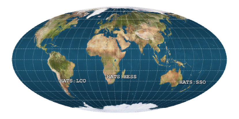
Figure 4.— Geographical location of the HATSouth sites on a Mollweide projection. These site provide near-optimal longitudinal separation, with LCO $\rightarrow$ SSO = $141\arcdeg$, SSO $\rightarrow$ HESS = $133\arcdeg$, and HESS $\rightarrow$ LCO = $86\arcdeg$. The three sites enable round-the-clock monitoring of selected southern stellar fields (image generated by xplanet).

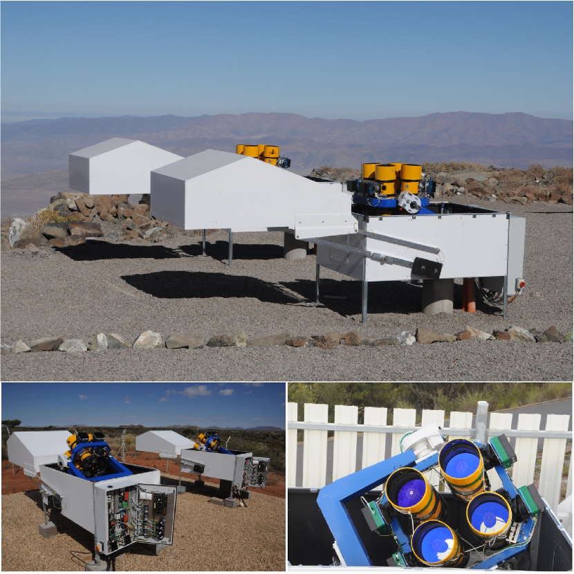
Figure 5.— The HS₄ units at Las Campanas Observatory, Chile (top), with the telescopes pointing towards the zenith. The HS₄ units at the HESS site in Namibia (bottom left), with telescopes stowed towards the south celestial pole. The electronic boxes are open showing the dome and telescope electronics described in § 2.1.5. A close-up view of an HS₄ unit at Siding Spring Observatory in Australia (bottom right), with part of the wind fence visible in the background.

The HATSouth network is operating at three premier astronomical sites in the southern hemisphere (Figure 4) that have a longitude coverage allowing for round-the-clock observations of nearly any celestial field in the southern hemisphere (that is close to the anti-solar point). The HS₄ units and control buildings were installed at all three sites in 2009, and the operations during 2009 predominantly involved commissioning of the network.

For the past two years, we have been continuously monitoring the meteorological conditions at the sites with 30 second time resolution using our weather sensing devices (§ 2.2). Of primary interest to us is the number of astronomically useful hours. By this we mean any time during the night when the weather server reports suitable observing conditions for our purposes. Based on monitoring during our commissioning period, suitable observing conditions exist only when:

1. The Sun elevation is below $-11\arcdeg$.

2. The sky temperature as measured by the Boltwood Cloud Sensor II is below $\sim-30\rm^{\circ}C\;$, indicating either cloud-free conditions or only thin, cold cirrus clouds. (The exact value has been adjusted depending on the site and the season.)

3. The average wind speed, as measured by the Vaisala weather-head in 30 s intervals, is below $13$ $\rm m\,s^{-1}$, in which case the amplitude of windshake will have a negligible effect on our image quality. Also, no gusts exceeding 18 $\rm m\,s^{-1}$occur.

4. The relative humidity as measured by the Vaisala weather-head is below 90%, which safeguards against dew condensing on the telescope front glass. Once the humidity exceeds 90%, it has to drop below 88% to declare the conditions suitable again.

5. The rate of lightning strikes as detected by the Boltek lightning sensor is below 50 strikes/min within 450 km of the site and less than 30/minute within 75 km, indicating there are no major electrical storms close to the site.

6. The precipitation rate as measured by the Vaisala weather-head is zero, indicating no rain, hail or snow.

We do not monitor atmospheric seeing, as our optical system delivers a stellar PSF of $\sim 10\arcsec$, which is much wider than the typical seeing at these sites ($\sim 1\arcsec$). We note that our criteria for suitable observing conditions relate critically to the specifics of our hardware and project. For example, other telescopes on the site may be able to operate at windspeeds and humidity levels above the HATSouth limits. Below we describe the three HATSouth sites, including their weather statistics (Fig. 7).

Chile

The Las Campanas Observatory (LCO) site ($70\arcdeg 42\arcmin 03.06\arcsec$ W, $29\arcdeg 00\arcmin 38.65\arcsec$ S) is located 110 km north-east of La Serena, Chile, and is operated by the Carnegie Institution for Science. LCO is famous for its extraordinary astronomical conditions, and hosts renowned telescopes, such as the twin 6.5 m Magellan telescopes, and the OGLE project, and will be the site of the future 25 m Giant Magellan Telescope (GMT). At 2285 m elevation, it has a dark sky and good transparency. The speed of the current network link requires us to manually ship most data back to the HSDC via Ultrium-4 800 GB tapes. There is very little seasonal pattern in the fraction of useful (clear) hours; the site is basically clear for most of the year. The yearly average of dark hours (Sun elevation $<-11\arcdeg$) is 10.2 hours. Based on two years of weather data (from 2010 March 15 until 2012 March 15), there are $\sim 8.48$ useful HATSouth observing hours per 24-hour period. Just 14% of the dark hours are cloudy, and only a further 3% of them not useful for reasons other than cloud (primarily high humidity or windspeed). The first two HS₄ units were installed at LCO in 2009 May, and operations started in 2009 July.

Figure 6.— Average number of dark hours for each site, broken down to useful (black), cloudy (light grey) or cloud-free but not useful (dark grey) due to other conditions (high humidity, wind, or lightning rate).

Namibia

The High Energy Spectroscopic Survey (HESS) site is located in the Khomas Highland (1800 m elevation) of Namibia, about 100 km south of Windhoek ($16\arcdeg 30\arcmin 10.17\arcsec$ E, $23\arcdeg 16\arcmin 23.32\arcsec$ S). Max Planck Institute for Astronomy (MPIA, Heidelberg, Germany) has access to the site through its partner institution, the Max Planck Institute for Nuclear Physics. Since the HESS project operates atmospheric Cherenkov detectors, the site was chosen for its very dark skies and good record of clear nights. There is a wet season from January through April, when the fraction of clear hours is significantly less than during the rest of the year. On average, we have $\sim 7.15$ useful HATSouth observing hours per 24-hour period at the HESS site. 26% of the dark hours are cloudy, with a further 5% not useful for reasons other than cloud (primarily high humidity or high lightning strike rates). We have a dedicated satellite-dish based Internet connection to the site with guaranteed 512 Kbit $\mathrm{s}^{-1}$ upload and download speed. This is marginally sufficient for monitoring the instruments and downloading the basic diagnostic plots. Similarly to the LCO site, data is shipped back via Ultrium tapes. The HS₄ units were installed to the site in 2009 August, and operations started shortly thereafter.

Australia

Siding Spring Observatory (SSO) is located in rural New South Wales in Australia ($149\arcdeg 03\arcmin 43.39\arcsec$ E, $31\arcdeg 16\arcmin 20.47\arcsec$ S). The site is owned and operated by the Australian National University’s (ANU) Research School of Astronomy and Astrophysics. SSO is the premier site for optical and infrared observation in Australia; it has excellent dark skies and substantial infrastructure, including a fast Internet link dedicated to research and training activities. Several Australian and international telescopes are located on the mountain, including the 3.9 m Anglo-Australian Telescope and the ANU’s 2.3m and SkyMapper telescopes. The ANU has permanent on-site technicians who can assist us if manual procedures are required. There is no strong seasonality in the fraction of clear hours. The typical wind conditions at the selected location for the HATSouth instruments necessitated building a wind-fence around the telescopes. This reduces windshake on the telescopes and ensures the dome hood can open and close without significant wind-load. High humidity, with otherwise clear skies and no wind, is more frequently an issue at SSO than at the LCO and HESS sites. The SSO site has had $\sim 4.64$ useful hours per 24-hour period over the past two years. 49% of the dark hours are cloudy, with a further 5% not being useful due to reasons other than cloud (primarily due to high humidity over the winter months). There is not much annual variation in the distribution of clear nights. We note that the current two-year statistics is certainly biased: based on annual rainfall records of the Australian Bureau of Meteorology, 2011 was the wettest year in Australia in the last century, and 2010 was among the top 10. The Internet connection between the HSDC in Princeton and SSO is very fast, reaching 40 Mbit/s both ways, which is high enough for us to transfer image data directly over the Internet without the need to ship tapes. The HS₄ units were installed in 2009 November, and operations started in 2009 December.

4.2. Scheme of nightly operations

The HS₄ units operate in a fully autonomous manner based on the vo (virtual observer) software (§ 3.1). The vo leaves its “daysleep” state an hour before sunset, and upon entering the “run” state, it starts cooling the CCDs and homes the mount. Whenever the photosensor permits, the vo opens the dome. The increased air-flow helps reaching a cooler set temperature for the CCDs, which in turn reduces CCD dark noise. The cameras are then kept at this fixed temperature during the entire night regardless of changes in the ambient air temperature so as to maintain CCD stability and ensure appropriate calibration frames are available for data reduction.

The vo starts the monfield task (our field monitoring program) when the Sun is at $-11\arcdeg$ elevation. All useful time between dusk and dawn (Sun elevation $<-11\arcdeg$) is spent executing the monfield task. For the purpose of selecting stars to monitor with HATSouth, we established a tiling of the entire sky consisting of 838 non-overlapping “nominal” fields, each $8\arcdeg\times 8\arcdeg$ wide. The HATSouth FOV is slightly larger than these fields, so by surveying them we gradually map the entire sky. We assign high priority to $\sim 12$ fields each year. These “primary” fields are chosen for observation based on several factors such as optimal visibility at the given time of the year, the expected sky density of dwarf stars, proximity of the field to Solar System objects, and prior history of observations. If none of the primary fields are visible for some reason, we select a field from a list of “secondary” fields. Our visibility calculations include distances from the Sun, Moon and bright Solar System planets, and constrain the zenith distance to be smaller than 60°.

Stability is of prime importance for maintaining high precision photometry. We make an effort to stabilize the positioning of the sources (astrometry), and the PSF of the sources (via focusing). Certain effects, however, are unavoidable; for example the differential refraction within the 8.2° field is 32″ at a zenith distance of 60°. The stellar profiles may also vary due to wind-shake.

4.3. Astrometric Stability

After each 240 s science frame we run “quick” astrometry on all four frames (originating from the four CCDs on the HS₄ unit), and adjust the position of the mount to track on the nominal field center. We typically achieve this to within 10″(rms). Astrometry is performed using the Two Micron All Sky Survey (2MASS; Skrutskie et al., 2006) catalog retrieved around the nominal position and a list of stars extracted from the image. The transformation between the two catalogs is determined using triangle matching, as described in Bakos et al. (2004) and Pál & Bakos (2006). Should this astrometry fail, we fall back on using astrometry.net (Lang et al., 2010), which can produce a robust (but less accurate) solution even for very large pointing errors. Failing astrometry is also an excellent diagnostic of various errors in automated operations, ranging from broken motors to poor initial orientation to the dome not opening. One unexpected effect we have noticed is “breathing” of the top frame holding the four telescope tubes, in the sense that the relative pointing of the four OTAs is a function of the hour angle (with an amplitude of $\sim 20\arcsec$).

4.4. PSF Stability

The stability of stellar PSF is maintained using a series of procedures. The encoder feedback and the RA TDM (§ 2.1.1) ensure accurate tracking, with no more than $\sim 1.2\arcsec$ positional change over four minutes exposure. Significant fork flexure at high hour angle can result in slightly elongated stars (primarily in the DEC direction), as the fork “unflexes” during the four minute exposure. We have quantified this effect for each HS₄ mount, and compensate for it by stepping the mount in DEC during the exposures. Also, we have developed an autofocusing routine to compensate for focus changes, due primarily to thermal effects adjusting the distance between the CCD cameras and the OTAs. First we take a series of frames with short (30 s) exposures, and adjust the focus in between the exposures. We then derive a map of the PSF parameters for each frame in this focus-series, and establish which frame exhibits the best focus. This is a non-trivial task due to the field curvature, CCD alignment, and the resulting variable PSF parameters across the field. We derive such a focus series once every two months. During normal field monitoring observations, we take a 30 s focus-frame every 3rd exposure. We derive the PSF map for the focus frame, and find the best match from our focus series. We then adjust the focus counter with the difference between the counter values for the best match and the originally established best focus. Short (30 s) exposures are required in order to minimize tracking errors, and fork flexure, and to decrease the effects of possible wind-shake, both for the initial focus series and for the regularly taken focus frames. The focus frames are not discarded, but instead are used for monitoring brighter stars that exceed their saturation limit by $\lesssim 2.3$ mag in the regular 240 s science frames.

The monfield task runs all night, taking 4 minute exposures, followed by $\sim 25$ s readout time and $\sim 12$ s time for astrometry and autofocusing. At the start of nautical twilight in the morning (Sun at $-11\arcdeg$ elevation) the vo starts taking skyflats in pre-selected regions close to the zenith, but always at least 40° away from the Moon. The skyflat task is terminated at around sunrise, at which point the dome is closed, and the vo launches the dark task which takes a series of 20 dark exposures of 240 s each. Finally the vo concludes the run by starting the bias task, which takes a series of 20 bias frames. The vo then enters “daysleep” state, the CCDs are warmed up to $\sim 0$$\rm{}^{\circ}C\;$(because in the daytime they would not be able to maintain the set temperature), and the vo waits for the the start of the next night.

Figure 7.— Observing statistics from the LCO, HESS and SSO sites. The top panel shows in light gray columns the good weather night-time hours for LCO as a function of date, since 2009 September. Dark gray columns show the actual hours spent with open shutters, averaged over the 8 CCDs per site. The panel immediately below shows the duty cycle, i.e. the ratio of the dark gray to light gray columns. The third and fourth panels show the same information for the HESS site, and the fifth and sixth panels refer to SSO.

4.5. Manual Interaction with the Telescopes

A number of software tools are available for manual interaction with the HATSouth control software components, notably with the virtual observer. These assume opening a secure shell (ssh) connection to the control computer. The software components can be started, stopped, restarted, or checked for operation. The weather status can be declared as inclement for operations, in which case, irrespective of the status shown by the weather sensors, the stations do not open up, but instead stay in daysleep or wthsleep state. This manual bad weather status can be issued when the user has advance information on e.g. a weather condition approaching the site (such as a storm system). We can query the detailed status of the observer, including information on the tasks scheduled, and the status of the individual hardware components.

The node computer on each site hosts a web-page that graphically displays the current and archival weather information in an easy-to-read format. The web-page also hosts the current and archival images from both the web camera that monitors the HS₄ units and the all-sky camera. Nightly movies are created from both these cameras and archived on the website. These webpages allow HATSouth team members across four continents to continuously check on both the weather conditions and operations at all three sites, and to make good decisions via manual intervention when conditions require.

4.6. Observing and operation statistics

Careful monitoring of the operational statistics is crucial for any automated survey. Such statistics can help in identifying and rectifying areas of the operation that are responsible for lost observing time. They can also reveal failing hardware components, and help in planning servicing missions to the sites, developing remote workaround solutions, or devising tests to clarify the nature of such failures. Surprisingly little is known of the operation statistics of automated surveys, and the reasons for failures are generally not documented.

Fig. 7 shows the weather and observing statistics for the three HATSouth sites. The light gray columns in Fig. 7 show the number of “useful” dark hours per night as a function of time for the past two years, where “useful” is defined to be when weather conditions meet the five criteria set out in § 4.1.

The number of hours the CCDs spent exposing on-sky per night are exhibited as dark gray bars in Fig. 7. If we had a 100% duty cycle, our total exposure time spent on-sky for science frames would be identical to the useful dark hours, i.e. the dark gray bars would perfectly match the light gray bars in Fig. 7. In reality, however, we lose time due to readout (25 s per frame), astrometry (12 s), and re-pointing of the telescope (2 s). Also, we take a bias frame after every 7 frames, and a 30 s focus frame after every 3 frames. Altogether, under ideal conditions, our duty cycle is 73%. We plot the actual duty cycle in Fig. 7 per night as a function of time for all three sites (the bottom parts of each panel, corresponding to the ratio of the dark gray to the light gray boxes). Chile, for example, is performing very stably at the 73% level. Higher duty cycle values were present in earlier stages of the project, when real-time astrometry and auto-focusing were not fully implemented. Consequently, the data quality during this “shake-down” period has been of lower quality.

The major reason for lower duty cycles has been due to ice crystals forming inside the chambers of many of the CCD cameras, which necessitated a lengthy process of returning them to the manufacturer for repair. Curiously, this only affected CCD cameras at the HESS (2011 April–July) and the SSO (e.g. 2010 March–July, and 2011 July–October) stations. Another serious cause of operational downtime was due to electronics being damaged by lightning storms both in Namibia and Australia, leading to about 1 month of time lost for each site. Other events that caused more limited downtime include: Internet outages (Namibia and Chile), instrument control software bugs, power outages (instruments shut down and not recovered, but the weather sensors operational), bush fire and excessive smoke (Namibia, Australia), cables chewed by rodents (Chile), and damaged printer port instrument control cards due to over-voltage. Also there is downtime during service missions, as we upgrade and test equipment.

In spite of the various failures presented above, the overall duty cycle of HATSouth has been very high. As of 2011 December 31, the HS₄ units opened up an average of 532 nights. We gathered $1\,060\,000$ $\rm 4K\times\rm 4K$ images at 4 minute integration time. Approximately 18 $8.2\arcdeg\times 8.2\arcdeg$ fields on the sky have been observed for an extensive time, accumulating more than $10\,000$ observations per field. Importantly we have never had an operational failure that resulted in a dome opening or remaining open in bad weather conditions which would compromise the safety of the hardware. We therefore believe the HATSouth operations strike the right balance between maximizing our duty cycle and minimizing the risk to the hardware.

5. Data flow and analysis

5.1. Data flow and data management

Many procedures relating to data have been carried over from the HATNet project, and have been described previously by Bakos et al. (2004) or Bakos et al. (2010). The most significant changes in the data of HATSouth with respect to HATNet are: i) a much larger overall data volume, ii) a more limited network bandwidth to the sites, iii) a more complex data structure due to the larger number of hardware components.

The HATSouth network creates a significant volume of data. Taking into account the fraction of useful hours for each site, HATSouth (all six HS₄ units) produces an average of 50 GB/day raw compressed data in the form of $\rm 4K\times\rm 4K$ FITS files. This corresponds to a rate of $\sim 150$ GB/day of calibrated, uncompressed (real) science frames from the network. The average yearly yield of the HATSouth network is 19 Terabytes (TB) of raw compressed pixel data, and 54 TB of calibrated science pixel data, plus $\sim 6.5$ TB of subsequent data products, such as photometry files and light curves.

On average HATSouth produces $\sim 20$ GB/day and 17 GB/day of raw, compressed data from our LCO and HESS sites respectively. Transferring these data to the HSDC in Princeton over the current Internet infrastructure is not feasible. We have therefore developed a scheme whereby each month the server computer writes this data to Ultrium-4 800 GB tapes. The tapes are then shipped to the HSDC in Princeton. Local help is needed to change tapes and ship them to the HSDC. This is, in fact, the only routine manual interaction needed to run the LCO and HESS sites. The situation is slightly different for SSO, where a gigabit data link between SSO and ANU in Canberra allows us to relatively simply transfer all raw, compressed data from SSO to the HSDC (averaging $\sim 13$ GB/day). We still write data to Ultrium-4 800 GB tapes at SSO for archival purposes, but regular shipping of these tapes is not required.

Figure 8.— The left panel shows the standard deviation of light curves around the median as a function of Sloan $r$ magnitude. The light (red) points refer to the fitted magnitudes (fitmag in § 5), and dark (blue) points refer to the TFA corrected tfamag values. Each point represents a light curve. The standard deviation has been corrected for the effect of using a number of template stars in the TFA fitting procedure. We use the optimal aperture (among three discrete choices) for each light curve, which choice is a function of the average magnitude of the star. We overplot the expected r.m.s. for each light curve, taking into account the expected photometric error for each observation within the light curve (calculated from the actual flux and sky background), and with scintillation noise (Dravins et al., 1998) added in quadrature to the noise term. We show the 10% (lowest), 50% (middle) and 90% percentile, as a function of magnitude, from the distribution of the expected r.m.s. The right panel shows the histogram of the number of stars in this particular (sparse) field with TFA r.m.s. smaller than 0.01 as a function of $r$ band magnitude (dark gray) and similar data for TFA r.m.s smaller than 0.02 (light gray).

Data management for HATSouth is non-trivial, as we are dealing with a large number of individual hardware components: 24 CCDs, 24 optical tubes, 6 HS₄ telescope mounts at 3 sites. Significant bookkeeping is required for distinguishing between these in the calibrations and subsequent data processing. For example, optimal processing of a light curve requires the knowledge of which hardware combination produced various subsets of the light curve. We also need to keep track of the time evolution of the components. Occasional servicing or fine-tuning of the system necessitates using a strict version control of the hardware. We thus maintain an extensive MySQL database describing all individual hardware components, along with their time evolution, expressed through version numbers. We illustrate this process by way of four examples.

1. If a CCD is returned for servicing, the gain, readout noise, bad pixel structure, cooling properties, and dark current structure may change, and calibrating pre-servicing data with post-servicing calibration frames (or the other way around) would be suboptimal. In such a case we thus introduce a new version number for the CCD, master bias, and master dark. Calibration is only permitted if version numbers match.

2. If a CCD is removed from the OTA, the filter is cleaned, and the CCD is installed back on the telescope, then the flatfield and pointing version numbers are incremented.

3. If a Takahashi optical tube requires re-alignment of the optical components, then the pointing model, flatfield version, and the PSF of the system will change, and a new focus series needs to be acquired.

4. If the telescope mount home proximity sensor is replaced, the pointing model of the system is incremented.

There is a long list of other possible hardware changes, ranging from the subtle (e.g. cleaning the telescope front glass) to the extreme (e.g. replacing CCD cameras). As long as the person servicing the telescope notes the changes in the central database, the pipeline will take them into account.

5.2. Data processing

Our data processing pipeline takes into account all of the data flow and data management considerations set out in § 5.1 to ensure an optimal calibration procedure. The pipeline has been developed in the python programming language. Routines where speed is an issue are written in C or C++. The pipeline is primarily run at the HSDC in Princeton. However the same pipeline, albeit with different sub-tasks, is also run on the on-site control and server computers.

Each control computer writes all FITS frames from its HS₄ unit’s CCD cameras to a directory created for that given night. Upon successful closing of the actual observing session by the vo (typically in the late morning, local time), that night’s image directory is “released”, and the calibration pipeline on the control computer is launched. It generates master bias, dark and flatfield frames for each CCD on the relevant HS₄ unit by combining the individual dark, bias and flatfield frames taken over the course of the night (average $\sim 30$ of each per night). Bias and dark master frames are the mean of the individual frames, after overscan correction and outlier pixel rejection. The master flatfield is a median average of the individual frames, after overscan, bias and dark corrections, and scaling the fluxes to the same median value in the center of the frame. Following this, all frames are transferred to our site server computer through the local network, thus providing an immediate backup of the data. The raw frames on the control computer are then compressed using a modified version of cfitsio/fpack, and are kept on the harddrives until they appear on our servers at the HSDC.

The site server computer produces a large variety of diagnostic plots for each HS₄ unit. Primarily these are plots of various telescope and image properties as a function of time or hour-angle. They are grouped by the image type (bias, dark, flat, object) or observed field. Examples of parameters plotted are pointing errors, focus positions, and the stellar profile. We also generate very small size, compressed (jpeg format) snapshots of selected regions of the science frames that can be readily transferred over the Internet for review. For certain diagnostics we need to perform on-the-fly calibrations using the on-site calibration master frames, however these on-site calibrated frames are deleted after the diagnostics have been determined. For all sites the master calibration frames, diagnostic plots, and observing logs (including MySQL database tables) are transferred to the HSDC each day, typically equating to $<500$ Mb of data transfer per site per day.

Due to the requirement to ship tapes from the LCO and HESS sites to the HSDC (see § 5.1), data arrives to the HSDC servers a few months after acquisition. Object frames are calibrated using the already transferred master calibration frames. Frames that have been successfully read-in from tape to our HSDC servers, and which have the same checksum as the original frames at the remote sites (checked via md5sum) are then purged from the remote site server and control computers. During the data transfer, we make sure that at least two copies of the data are kept at any given time (including data on the tapes).

The rest of the data processing takes place on the HSDC computer cluster at Princeton University. While “quick-astrometry” was already run on the frames during observations (§ 4.2), we refine the astrometric solutions using more time intensive procedures. Should the astrometry fail to find a solution for a frame, we exploit the astrometric information from the neighboring CCDs (with known geometrical offsets). The astrometry uses sixth order polynomial fits between pixel coordinates and the 2MASS catalog. We then perform aperture photometry at the fixed positions of the 2MASS stars in a series of apertures. Aperture photometry in 3 fixed radius apertures is performed with tools originally developed as part of the HATNet project (Pál, 2009b; Bakos et al., 2010), and modified for our purposes. Photometry and subsequent data products are kept in binary format to minimize storage requirements and improve performance in file I/O operations.

Basic variations in the photometry due to extinction, changing PSF size in the fixed aperture, etc., are removed by calibrating the photometry of individual frames to the photometry of a reference frame. This reference is selected to be a frame taken under dark and transparent sky conditions, and having the median FWHM of the other images. The procedure is done in an iterative way, excluding stars which display significant brightness variations after applying the magnitude transformation, as determined from a large ensemble of stars. Such variation might indicate the star is undergoing actual astrophysical variability. Stars are weighted by their individual formal photometric errors in this fitting procedure. After performing this correction to all observations of a given field, a new reference frame is generated by combining all corrected magnitudes, and the process is repeated by using the r.m.s. of their preliminary light curves as weights.

5.3. Light curves

We start with $\mathcal{O}(10^{4})$ magnitude-fitted photometry files (one for each frame) for a given field and CCD. Each photometry file has photometry information for each of the $\mathcal{O}(10^{4})$ sources in the frame. The photometry files are then transformed into light curves (information per source with $\mathcal{O}(10^{4})$ observations), while retaining the binary format. The fitted magnitude light curves (called fitmag light curves) have remaining trends removed by decorrelating against external parameters (resulting in epdmag light curves) (Bakos et al., 2010) and then using the Trend Filtering Algorithm (yielding tfamag light curves) (TFA; Kovács et al., 2005).

For the brightest non-saturated stars, the resulting light curves typically reach a per-point photometric precision of $\sim 6$ mmag r.m.s. around the median at 4-minute cadence. These light curves combine data from three different HS₄ units, one each at LCO, the HESS site, and SSO. The distribution of r.m.s. values is shown in Fig. 8 (left panel), where red (light) points show the r.m.s. of the fitmag light curves, and black (dark) points exhibit the r.m.s. of the final tfamag light curves. Each of the $\sim 27000$ points represent a light curve with $\sim 8000$ observations, taken from a moderately sparse field at galactic latitude $-40\arcdeg$. Observations were contributed by all three HATSouth sites. The standard deviation has been “unbiased” so as to correct for the effect of fitting the light curve with $\mathcal{O}(10^{2})$ coefficients (the number of template stars) in the TFA procedure. Clearly, the detrending procedures significantly decrease the r.m.s. values of the light curves. Theoretical estimates have also been overlaid in Fig. 8 as solid lines. In the left panel we show the 90th, 50th and 10th percentile curves for the expected r.m.s., as calculated from the photon and sky background noise values for each individual measurement, and an overall scintillation noise (Dravins et al., 1998) added in quadrature. That is, we expect 90% of the r.m.s. values would lie under the solid line on the top with these noise sources included in the overall noise budget. We are working on clarifying and trying to rectify the discrepancy between the expected and observed scatters of the light curves. There is room for improvement, and we believe that a major contribution to this discrepancy may be due to the complex sub-pixel structure of the microlensed and dual-gate front-illuminated pixels (§ 2.1.3), coupled with the anti-blooming effect, and the relatively narrow PSF. These effects appear to be not very well corrected by the EPD and TFA procedures. The right panel of Fig. 8 shows a histogram of stars in 0.2 mag bins as a function of $r$ band magnitude for stars having r.m.s.$<0.01$ and $<0.02$, respectively. The sub-percent r.m.s. actually attained for stars with $r<13.25$ allows us to achieve the primary science goal of HATSouth, namely the discovery of transiting hot Jupiters, and even Neptune-size planets (given the large number of data-points per field, and the often uninterrupted time-series). Figure 9 shows light curves for four representative variable stars identified from the HATSouth light curves.

Figure 9.— Phased HATSouth light curves for four representative variable stars identified from the observations obtained to date. These include a $P=37.9$ d periodic variable (upper left), a $P=0.24$ d periodic variable (upper right), a $P=1.4$ d transiting hot Jupiter (lower left), and a $P=16.6$ d transit candidate. The upper two examples are epdmag light curves (see § 5.3) with arbitrary reference phases, the lower two are tfamag light curves and are displayed with the transits at phase 0.5.

5.4. Transit search

We search the tfamag light curves for periodic transit events using the Box-fitting Least Squares algorithm (BLS; Kovács et al., 2002). We then subject potential transit candidates to a number of automatic filters to select reliable detections which are consistent with a transiting planet-size object, and are not obviously eclipsing binary star systems or other types of variables. For example, we constrain the maximum depth of the transit ($\lesssim 0.1$ mag), we require at least two transit events with altogether at least $50$ data-points in transit, we limit the maximum radius of the transiting object to be $\lesssim 2$ $R_{\rm J}$ (based on the transit depth, and assuming a zero-age main sequence host star with stellar radius estimated from the $J-K$ color index). We also check for the difference in $\chi^{2}$ between the best fit transit model, and the best fit model where even and odd transits are allowed to have different depths. The maximum gap in the phased light curve is also limited to be $\sim 0.2$. We note that the exact selection criteria may depend on the field, and we may perform multiple runs of automatic selections with different criteria. Altogether, the result is a machine-generated list of candidate TEP hosts, including relevant light curve details (period, apparent transit depth, etc.). The automated transit candidate selection procedure provides a manageable list of potential candidates which must then be inspected by eye to select and prioritize the most promising targets for follow-up. Typically a few hundred to one thousand potential candidates per $8.2\arcdeg\times 8.2\arcdeg$ field are identified by the automated procedures, which are then winnowed by hand to several dozen candidates per field deemed worthy of follow-up. First, the properties of the light curve are analyzed, such as its BLS frequency spectrum, alternate folding periods, out-of-transit variations, light curves of neighboring stars, appearance after running TFA with alternate templates, etc. In addition, a variety of resources are consulted, including archival plates, 2MASS digital archives, appearance on HATSouth frames, proper motions, and catalogs available through CDS/Vizier. At the end of this phase, relative priorities are assigned to surviving candidates and appropriate facilities for follow-up are identified.

6. Expected performance

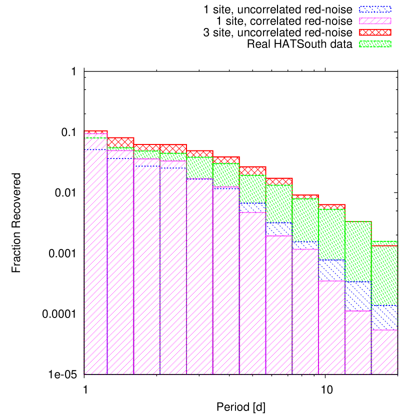
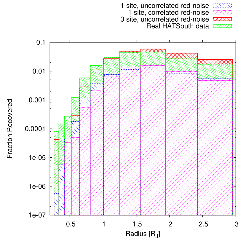
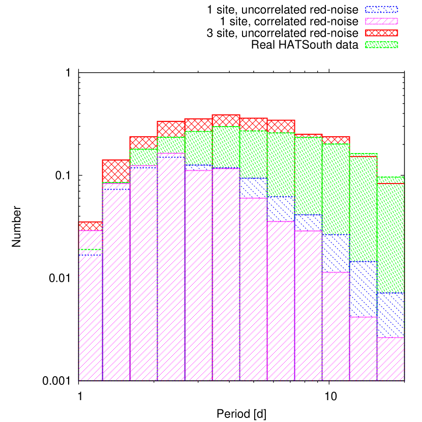
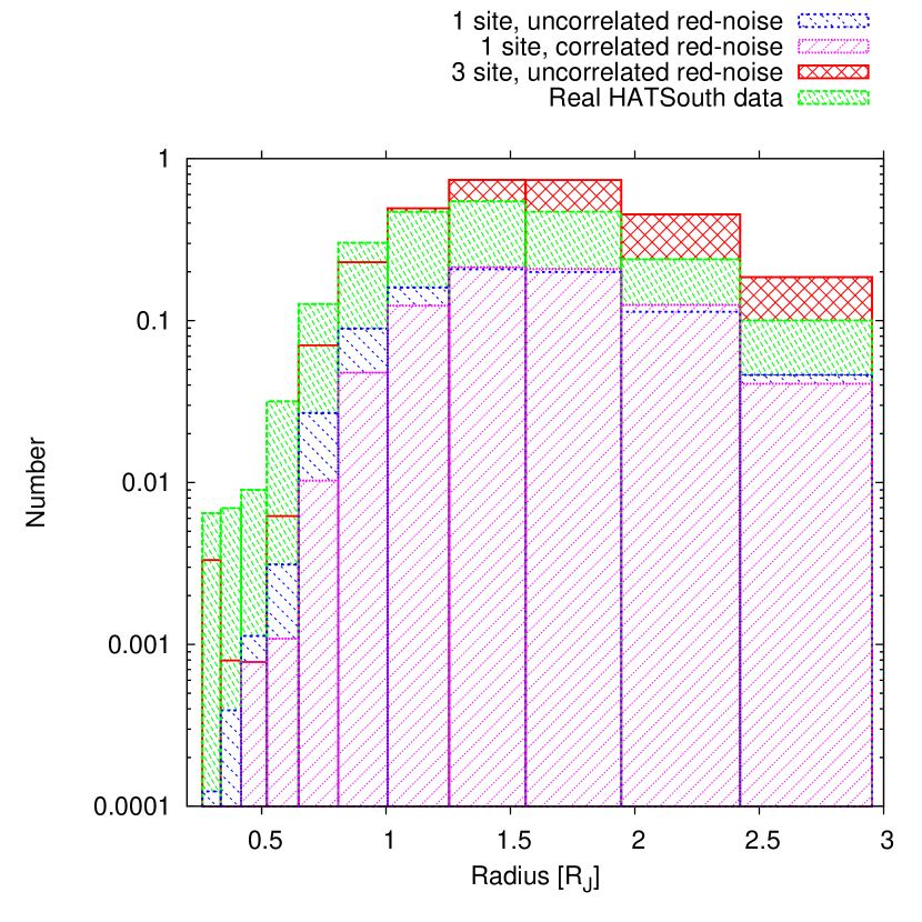
Figure 10.— The expected recovery rate of transiting planets as a function of period (upper left) and radius (upper right), marginalized in each case over the other parameter. Note the logarithmic scales. The recovery rates are displayed for the four sets of transit injection/recovery simulations listed in Section 6 (see the figure key; they are in the order of scenarios 1 through 4). These are combined with the intrinsic planet period and radius distributions, and corrected for the geometric transit probability, to determine the expected planet yield for a single HATSouth field as described in Section 6. We show the yield as a function of period (lower left) and radius (lower right).

In order to estimate the expected yield of transiting planets from the HATSouth survey we conduct transit injection and recovery simulations, following the procedure summarized below (see also Burke et al., 2006; Hartman et al., 2009a; and Bayliss and Sackett, 2011). Additional details are provided in Appendix A.

1. Use the Besançon Galactic model (Robin et al., 2003) to simulate a sample of stars which we might expect to observe in a typical HATSouth field.

2. Use the results from Howard et al. (2011), based on the Kepler mission, to determine the underlying joint distribution of planet periods and radii over the ranges of HATSouth sensitivity. This is a fundamental distinction from most previous attempts to estimate the expected planet yield of a transit survey where the planet distribution was either taken to be unknown, or was assumed to be constant over the period and radius ranges surveyed.

3. Generate a time-base (i.e. a set of observation times to use for the light curve simulations) resulting from a two-month observing campaign. This is generated taking into account the field visibility from each site, the exposure times and overheads, and the empirical weather statistics for each site.

4. Draw $>5\times 10^{5}$ samples from the above stellar and planetary distributions.

5. For each sample simulate a light curve with an injected transit. The light curve is generated with white and red noise appropriate for the magnitude of the star, with quadratic limb darkening parameters from Claret (2004) appropriate for the stellar atmospheric parameters, random transit phase, and with $\cos i$ uniformly distributed between $0$ and $(R_{\star}+R_{P})/a$ (i.e. we assume a uniform distribution of orientations for the orbits, with the condition that transits must occur). We assume circular orbits.

6. Apply the BLS and candidate selection algorithms used in the HATSouth search § 5.3 to the simulated light curves to recover the transits.

7. Based on the recovery rate, the geometric transit probability for each simulation, and the total fraction of stars with planets from Kepler within the period and radius ranges used for our simulations, determine the total expected planet yield as a function of planet period and radius.

We execute the above procedure four separate times for the following scenarios:

1. Three imaginary HATSouth instruments at a single site (we choose LCO as the site with the optimal weather statistics), red noise is uncorrelated between the instruments.

2. Three HATSouth instruments at a single site, red noise is correlated between the instruments.

3. One HATSouth instrument at each of the three sites. This simulates the actual configuration of HS₄ units (even though the real setup has two units per site), using a generated time-base and simulated light curves with appropriate noise parameters.

4. Transits are injected into actual HATSouth light curves for a field observed by 1 HATSouth instrument at each of the three sites over a two-month time-span.

The results from these simulations are shown in Figure 10. We plot the transit recovery rate both as a function of period and of planet radius (i.e. the fraction of transiting planets with a given period or radius that would be recovered by HATSouth), and the expected planet yield for a single HATSouth field (that is, the above, weighted by the actual occurrence rate of planets). The recovery rates and yields are shown for each of the four scenarios listed above. We find that for a single HATSouth field observed over two months the total expected planet yield is $0.85$, $0.77$, $2.9$ or $2.3$ planets for scenarios 1 through 4, respectively (by total we mean integrated over all radii and all periods). These results clearly show the significant increase in the expected planet yield by using a global network (simulations 3 and 4); a three site global network has an expected planet yield that is $>\!3$ times larger than the simulations where all of the instruments are kept at a single site (simulations 1 and 2). Assuming 12 fields observed per year, we expect to find $\sim 30$ transiting planets per year with HATSouth, including $\sim 1$ planet per year with $R\!<0.7\,R_{J}$ and $\sim 6$ planets per year with $P>10$ d. These numbers could be significantly improved by reducing the instrumental red noise. Of course, the final number of planets heavily depends on the follow-up time invested in confirming these candidates; this estimate assumes all candidates are followed up.

The expected $\sim 1$ planet per year with $R\!<0.7\,R_{J}$ could be a Neptune-mass, or even a super-Earth mass planet. It is worth noting that the unique sensitivity (among ground-based transit searches) to periods longer than 15 days opens up the possibility of finding transiting super-Earths with orbits within the Habitable Zone surrounding a mid-M dwarf. Thus, a super-Earth orbiting an M5 dwarf ($M_{\star}\sim 0.21\,M_{\sun}$; $R_{\star}\sim 0.27\,R_{\sun}$) at or slightly greater than a distance of 0.07 AU, which corresponds to the inner edge of the star’s Habitable Zone (Kasting, Whitmire, & Reynolds, 1993), would have an orbital period of about 15 days or a little longer, well within the reach of the HATSouth survey (Fig. 10).

7. Conclusions

HATSouth is the world’s first global network of identical and automated telescopes capable of 24-hour observations all year around. The telescopes are placed at three southern hemisphere sites with outstanding observing conditions (LCO in Chile, HESS site in Namibia, SSO in Australia). Long stretches of continuous observations are often achieved. Fig. 11 shows the contiguous blocks of clear weather periods as a function of Julian Date for the past two years. The longest uninterrupted clear period, based on the detailed weather logs for each of the three sites, is 130 hours long. Relatively long stretches, exceeding 24 hours, are quite frequent.

HATSouth builds on the successful northern hemisphere HATNet project (Bakos et al., 2004). However, it implements numerous changes with respect to HATNet. Broadly speaking, we reach into a fainter stellar population, having many more dwarf stars per square degree, thus increasing our overall sample, and also having more dwarfs relative to giant stars (which dilute the sample). The fraction of K and M dwarfs is also significantly higher, facilitating more efficient detection of smaller planets, such as super-Earths.

Each of the three sites hosts two HATSouth instruments, called HS₄ units. Each HS₄ unit holds four 0.18 m, fast focal ratio hyperbolic astrographs, tilted $\sim 4\arcdeg$ with respect to each other to produce a mosaic image spanning $8.2\arcdeg\times 8.2\arcdeg$ on the sky, imaged onto four $\rm 4K\times\rm 4K$ CCD cameras, at a resolution of 3.7$\rm\arcsec pixel^{-1}$. The photometric zero-point is $r\approx 18.9$ (meaning 1 ADU/s flux), and the 5-$\sigma$ detection threshold for the routinely taken 240 s images is $r\approx 18.5$. Stars become saturated at $r\approx 10.5\pm 0.5$ in the 240 s exposures, depending on the focus (thus width of the stellar profile), and the degree of vignetting at the position of the star. We also monitor stars as bright as $r\approx 8.25$ using shorter exposure (30 s) images.

Meteorological conditions are monitored by a weather station (wind, humidity, temperature, precipitation), a cloud detector (primarily cloud cover), a lightning detector (forecasting lightning storms), and an all-sky fisheye camera, all installed on our HATSouth control building. In addition, the individual HS₄ units are aided by a hardwired rain detector and a photosensor (for avoiding daytime opening of the dome). Each HS₄ unit is controlled by a single rack-mounted computer running Linux and Xenomai. We have developed a dedicated software environment for operating the telescopes, including all hardware components, such as the dome, telescope mount and CCDs. Virtual Observer (vo) is the intelligent software, managing all aspects of running the observatory, such as preparing devices, scheduling observations, monitoring the weather, handling exceptions, communicating with the outside world, and logging events and observations.

The network monitors selected fields on the southern sky for about 2 months per field. Fields are selected in a way that all dark time during the night is used. A significant effort is made to optimize the data quality, by re-focusing the optics every $\sim 15$ minutes, running real-time astrometry after the frames, and adjusting the pointing of the mount.

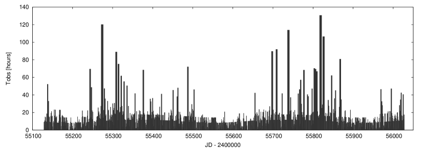
Figure 11.— Contiguous good weather stretches as a function of Julian Date. The height (and width) of the boxes represent the number of dark hours that were clear from either of the LCO, HESS or SSO sites without an interruption. Any bad weather longer than 10 minutes in duration is considered as an interruption. The longest stretch of clear period was about 130 hours (5.4 days) long.

This combination of precise weather monitoring, the use of a very stable operating system, and running a dedicated software environment has resulted in very robust operations. Indeed, the HATSouth network has taken over 1 million $\rm 4K\times\rm 4K$ science frames during its initial 2 years of operations. The six HS₄ units have each opened up an average of $\sim 500$ nights so far, without a single case of opening when weather conditions were not suitable.

We have developed a scheme that reduces the amount of data transferred from the remote sites to the HSDC in Princeton. The reduction pipeline keeps track of the large number of individual hardware components (24 OTAs, 24 CCDs, etc), and maintains a version control for the above, since hardware may change due to routine maintenance or instrument repairs. The current reduction procedure, after application of the Trend Filtering Algorithm (TFA Kovács et al., 2005), yields light curves reaching 6 mmag r.m.s. at 240 s cadence at around the saturation limit. The light curves are searched for transit candidates using a well-established methodology that has been developed for HATNet, and relies on the BLS (Kovács et al., 2002) algorithm and post-processing. The network is producing high quality planetary transit candidates, and general variability data (Fig. 9). Follow-up observations for these candidates are being performed as an intensive team-effort, and will be described in subsequent publications.

We have run detailed, realistic simulations on the expected yield of transiting planets from the HATSouth network. The simulations take into account the noise characteristics of the instruments, the weather pattern, the observing windows, the stellar population, the expected planetary population based on recent Kepler results, and our search methodology for transits. We compared two basic scenarios: all HS₄ telescopes are at a single site and observing the same field at higher S/N, or the telescopes are spread out to the current setup, and observe the same field at lower S/N (per unit time), but at much higher fill-factor. The simulations were performed both with uncorrelated and correlated “red”-noise components in the light curves. The results clearly prefer the networked setup, predicting a three-fold increase in the number of detected transiting planets, as compared to a single site setup. The long stretches of observations (Fig. 11), and uncorrelated noise between the stations, are clearly fundamental in this increased yield. Notably, the fraction of planets recovered at $P\approx 10$ d period is about 10 times that of a single-site installation (Fig. 10, top left panel), and the planetary yield after taking into account the Kepler distribution of planets and the geometric transit probability is also $\sim 10$ times higher than for the single-site installation (Fig. 10, bottom left panel). The peak sensitivity occurs at $P\approx 6$ days (marginalized over all planetary radii), and exhibits much slower decline towards long periods than the single-site setup. Similarly, there is a significant increase (factors of 3 to 10) in the detection efficiency as a function of planetary radius, especially at small radii. The peak sensitivity, however, occurs at $\sim 1.5\,R_{\rm J}$ for both the networked and single-site setups. Altogether, we expect that HATSouth is capable of the detection of $\sim 30$ transiting extrasolar planets per year, pending follow-up confirmation of these candidates.

Note that while the HATSouth stellar sample is somewhat fainter than that of HATNet, the candidates are still within the reach of follow-up resources available in the southern hemisphere. Examples for such spectroscopic follow-up resources (including those with reconnaissance or high precision radial velocity capabilities) are the Wide Field Spectrograph (WiFeS; Dopita et al., 2007) on the ANU 2.3 m telescope, FEROS on the MPG/ESO 2.2 m telescope, CORALIE on the Euler 1.2 m telescope, HARPS on the ESO 3.6 m telescope (all at La Silla, Chile), the Echelle spectrograph on the 2.5 m du Pont telescope at LCO, and the UCLES spectrograph on the 3.9 m AAT at SSO.

Global networks of telescopes present a powerful way of studying time-variable astronomical phenomena. By coupling this with telescopes that are identical and fully automated, it is possible to undertake large, long duration surveys that would have been completely unfeasible with manually operated or single site facilities. HATSouth is the first of many projects that will utilize the combination of these two concepts over the next decade and, we hope, make many exciting discoveries in the process.

Acknowledgements

Hardware costs for the HATSouth project were funded by NSF MRI grant NSF/AST-0723074. Construction of the infrastructure at the HESS site was funded by MPIA, and similar costs at SSO enjoyed partial funding from the ANU. We thank the Smithsonian Astrophysical Observatory for the Internal Research and Development (IR&D) funds that supported visiting students Gábor Kovács and Zoltán Csubry during the 2008–2009 development phase of the project. Following the installation and calibration, the overall operation of the HATSouth network has been supported by NASA grant NNX09AB29G.

We wish to thank directors Wendy Freedman (Carnegie – Las Campanas Observatory), Miguel Roth (Las Campanas), Harvey Butcher (ANU – Siding Springs Observatory), and Werner Hofmann (MPIK – HESS site) for their generous support towards accommodating the HATSouth instruments at the respective sites. Our home-base for development, procurement, installation, and early operation of the HATSouth network was at the Smithsonian Astrophysical Observatory. We greatly appreciate the outstanding support of SAO director Charles Alcock, and associate directors Nancy Brickhouse and Roger Brissenden. We also thank Matt Holman for his help in the initial phase of the project.

Installation to the respective HATSouth sites required team-work in a hectic schedule. We thank F. Rózsa for joining our installation team to Namibia and Australia. At Las Campanas, we are indebted to the whole staff for their help in installation, and particularly so to Francisco Figueroa, Marc Leroy, Juan Espoz, Juan Espoz, Jr., Andrés Rivera, Patricio Pinto, and Henry Cortes for their very generous support. Don Hector and the kitchen staff at LCO provided delicious meals that kept us going through the long installation days. We also thank Earl Harris (Carnegie) for his assistance in the transportation of telescope components to the site. At the HESS site, we are most grateful for the help of Toni Hanke, site manager, technical support Albert Jahnke, and our hosts Adele and Joachim Cranz. We greatly benefited from discussions with Michael Panther and German Herman (MPIK) in the initial planning phase of the project. At ANU’s Siding Springs Observatory, we thank Geoff White for his help during installation and the first two year’s of operation. Tammy Roderick at ANU helped identify many issues in relation to the first set of HATSouth images and we thank her very much for her contribution to the project. We greatly appreciate the help we received from Gabe Bloxham at ANU in relation to the telescope optics. We also thank Colin Vest at ANU for his help in servicing the Australian telescopes. We appreciate Vince O’Connor’s help in administrative matters regarding the installation. G.Á.B. was supported as an NSF Fellow (AST-0702843) by SAO during the development of this project. G.Á.B. is extremely thankful for the family of P. Sári for hosting and operating the prototype instrument in their garden at Pécel, Hungary, for an extended period of almost one year. G.Á.B. also wishes to thank the SAO administration for the swift management of the relevant grants, in particular to P. Sozanski, J. Lendall, N. Rathle, L. Linarte and E. Dotts. We thank T. Szklenár for his expert help in the system management of computers during 2011 at the remote sites and at Princeton. We also thank Gy. Medgyesi for his help in the mechanical design of the HATSouth units. We thank P. Jónás and his family for their help in the Australian installation. A.J. acknowledges support from Fondecyt project 1095213, Ministry of Economy ICM Nuclei P07-021-F and P10-022-F, Anillo ACT-086, BASAL CATA PFB-06 and FONDAP CFA 15010003. V.S. acknowledges support form BASAL CATA PFB-06. M.R. has been supported by ALMA-CONICYT projects 31090015 and 31080021, and by a FONDECYT postdoctoral project 3120097. G.K. is supported by RoPACS, a Marie Curie Initial Training Network funded by the European Commission’s Seventh Framework Programme.

Appendix A Details of the Planet Yield Simulations

The general procedure that we follow to determine the expected planet yield with HATSouth is outlined in Section 6, here we provide additional details concerning this procedure.

We use the online Besançon Galactic model simulator to generate a sample of stars observed in a typical HATSouth field centered at coordinates $\alpha=300^{\circ}$, $\delta=-22.\!\!^{\circ}5$, which is at $b=-24.\!\!^{\circ}6$ Galactic latitude. Importantly, this model gives both physical parameters (mass and radius) and observed parameters (magnitudes in various passbands) for each star, which are needed to simulate the transit light curves.

We use the underlying planet period and radius distribution from Howard et al. (2011, hereafter H11). This includes Equation 4 from H11 for the planet radius distribution:

$$\frac{{\rm d}f(R)}{{\rm d}\log R}=k_{R}R^{\alpha}$$ (A1)

with $\alpha=-1.92\pm 0.11$ and $k_{R}=2.9^{+0.5}_{-0.4}$ for planets with $P\!<\!50$ d, and Equation 8 from H11 for the planet period distribution:

$$\frac{{\rm d}f(P)}{{\rm d}\log P}=k_{P}P^{\beta}\left(1-e^{-(P/P_{0})^{\gamma}}\right)$$ (A2)

with values for $k_{P}$, $\beta$, $P_{0}$ and $\gamma$, which depend on the planet radius, taken from Table 5 of H11. They found that 16.6% of GK dwarf stars have planets in the range $P\!<\!50$ d and $2\,R_{\earth}\!<\!R\!<\!32\,R_{\earth}$. We restrict our simulations to the range $P\!<\!20$ d and $3\,R_{\earth}\!<\!R\!<\!32\,R_{\earth}$. Integrating the H11 distribution over the restricted ranges yields a planet occurrence frequency of 1.73%. This is used, together with the geometric transit occurrence probability for each planet, the total number of stars observed in the field, and the total number of fields observed by HATSouth per year, to scale the recovery frequency from our simulations to determine the expected yearly planet yield from HATSouth.

In drawing samples of stars and associated planets we assume that the stellar and planet distributions are independent. This is known to be a false assumption when considering stars over the spectral range from M to A (e.g. Johnson et al., 2011). However, the distribution of spectral types for the dwarf stars observed by HATSouth is expected to be fairly similar to that observed by Kepler, with perhaps a slight bias towards hotter stars in HATSouth given the brighter magnitude limits of the survey. Because the occurrence of massive planets on close-in orbits increases for hotter stars, assuming the Kepler planet distribution applies for all stars in the HATSouth survey most likely underestimates the total number of planets to which HATSouth is sensitive.

We follow two approaches to generating light curves with realistic noise properties. One approach is to simply use the real (observed) light curves (simulation 4 in Section 6) choosing for each simulated star the observed star from a given field that is closest to the simulated star in magnitude. The other approach is to simulate a light curve with both white and red noise (simulations 1 through 3 in Section 6). To do this we follow the wavelet-based procedure given in Section 4.2 of McCoy and Walden (1996) (see also Carter and Winn, 2009) to generate a uniformly sampled time-series with $\sim f^{-0.99}$ red noise using the publicly-available Vartools program (Hartman et al., 2008). This time series is then interpolated onto the time-base of the simulated observations, and scaled to have a standard deviation of $5$ mmag (our conservative estimate of the red-noise in the HATSouth light curves). To this light curve we add Gaussian random noise with standard deviation equal to the expected light curve standard deviation, based on the photometric errors (including photon noise from the star, sky noise, and read-noise), of the observed star from a given field that is closest to the simulated star in magnitude.

We use Vartools to inject Mandel and Agol (2002) model limb-darkened transit light curves into the simulated light curves. We assume only one transiting planet per star. Before injecting the transits we dilute the model signal by a factor of 0.8 which, based on our experience with HATNet, is the typical factor by which the TFA detrending algorithm, as applied to the HATSouth light curves, reduces the transit depths. We then apply BLS at the fixed period of the injected transit to determine the S/N of the transit in the light curve. In the great majority of cases the transits are much too shallow relative to the light curve noise to have any hope of detecting them (the stellar distribution increases towards fainter stars, while the planet distribution increases towards smaller radius planets on longer period orbits), we therefore use this quick cut on the S/N of the injected transit to immediately reject undetectable transits without executing the full BLS transit search, and reserving the computationally expensive search only for those simulations for which there is some chance that the transit could be recovered.

To simulate as closely as possible the HATSouth survey, as executed, we apply the same BLS search, peak identification, and automated candidate selection routines to the simulations passing the aforementioned S/N cut as we apply in the actual survey. The selection routines are applied to the top five peaks in the BLS spectrum of a light curve. To consider a simulation to be recovered we further require that one of the peaks that passes the automated selections corresponds to a frequency that is within $0.02$ d^-1 of the injected frequency. To account for the possibility that our by-eye selection of candidates rejects real planets which pass the automatic selections, we inspected by eye a randomly selected subset of the simulations which passed the automatic cuts. As a control, we mixed into this subset a random sample of simulated light curves for which the injected transit was not recovered, but for which a significant peak was identified in the BLS spectrum. We found that 95% of the automatically recovered transits also passed the by-eye selection (ranging from about 70% of the simulations with S/N near the cut-off value, to 100% of the simulations with S/N$>$12.5), while 90% of the non-recovered transits were rejected by our by-eye selection.

The total expected yearly yield of planets with periods between $P_{\rm min}\!<\!P\!<\!P_{\rm max}$ and radii between $R_{\rm min}\!<\!R\!<\!R_{\rm max}$ is given by:

$$N(P,R)=\frac{N_{\rm obs}}{N_{\rm sim}}f_{\rm tot}\sum_{i=1}^{N_{\rm sim}}\theta(R_{i}-R_{\rm min})\theta(R_{\rm max}-R_{i})\theta(P_{i}-P_{\rm min})\theta(P_{\rm max}-P_{i})\delta_{i}f_{\rm eye}(SN_{i})\frac{R_{\star,i}+R_{i}}{a_{i}}$$ (A3)

where $N_{\rm obs}$ is the number of dwarf stars expected to be surveyed per year (given by the number of dwarf stars in the Besançon simulation, times 12 fields observed per year), $N_{\rm sim}$ is the number of simulations conducted, $f_{\rm tot}$ is the total fraction of stars with planets within the period and radius ranges of the simulations (1.73%), and the sum is over all simulations, with $\theta(x)=1$ for $x>0$, $\theta(x)=0$ for $x\!<\!0$, $\delta_{i}=1$ if the simulated transit is recovered and $0$ if not, $f_{\rm eye}(SN_{i})$ is the fraction of automatically selected candidates with transit S/N$\sim SN_{i}$ that pass the by-eye selection, and $(R_{\star,i}+R_{i})/a_{i}$ is the geometric probability of transit for simulation $i$.

References

- Albrow et al. (1998) Albrow, M., et al. 1998, ApJ, 509, 687
- Akerlof et al. (1999) Akerlof, C., Balsano, R., Barthelmy, S., et al. 1999, Nature, 398, 400
- Akerlof et al. (2003) Akerlof, C. W., Kehoe, R. L., McKay, T. A., et al. 2003, PASP, 115, 132
- Alonso et al. (2004) Alonso, R., Brown, T. M., Torres, G., et al. 2004, ApJ, 613, L153
- Baglin et al. (2006) Baglin, A., Auvergne, M., Boisnard, L., et al. 2006, 36th COSPAR Scientific Assembly, 36, 3749
- Bakos et al. (2002) Bakos, G. Á., Lázár, J., Papp, I., Sári, P., & Green, E. M. 2002, PASP, 114, 974
- Bakos et al. (2004) Bakos, G. Á., Noyes, R. W., Kovács, G., Stanek, K. Z., Sasselov, D. D., & Domsa, I. 2004, PASP, 116, 266
- Bakos et al. (2010) Bakos, G. Á., et al. 2010, ApJ, 710, 1724
- Batalha et al. (2012) Batalha, N. M., Rowe, J. F., Bryson, S. T., et al. 2012, submitted to ApJS, arXiv:1202.5852
- Bayliss and Sackett (2011) Bayliss, D. D. R., & Sackett, P. D. 2011, ApJ, 743, 103
- Borucki et al. (2010) Borucki, W. J., Koch, D., Basri, G., et a. 2010, Science, 327, 977
- Boyd et al. (1984) Boyd, L. J., Genet, R. M., & Hall, D. S. 1984, International Amateur-Professional Photoelectric Photometry Communications, 15, 20
- Brown et al. (2010) Brown, T. M., Burleson, B., Crellin, M., et al. 2010, Bulletin of the American Astronomical Society, 42, #441.06
- Burke et al. (2006) Burke, C. J., Gaudi, B. S., DePoy, D. L., & Pogge, R. W. 2006, AJ, 132, 210
- Carter and Winn (2009) Carter, J. A., & Winn, J. N. 2009, ApJ, 704, 51
- Castro-Tirado (2010) Castro-Tirado, A. J. 2010, Advances in Astronomy, 2010,
- di Ciccio (2011) di Ciccio, D. 2011, S&T, October, 60
- Claret (2004) Claret, A. 2004, A&A, 428, 1001
- Dravins et al. (1998) Dravins, D., Lindegren, L., Mezey, E., & Young, A. T. 1998, PASP, 110, 610
- Dong et al. (2009) Dong, S., Bond, I. A., Gould, A., et al. 2009, ApJ, 698, 1826
- Dopita et al. (2007) Dopita, M., Hart, J., McGregor, P., Oates, P., Bloxham, G., & Jones, D. 2007, Ap&SS, 310, 255
- Filippenko et al. (2001) Filippenko, A. V., Li, W.‘D., Treffers, R. R., & Modjaz, M. 2001. In Small-Telescope Astronomy on Global Scales, ed. W. P. Chen, C. Lemme, and B. Paczyński (San Francisco: Astron. Soc. Pacific, Conf. Ser. Vol. 246), 121-130.
- Gould et al. (2010) Gould, A., Dong, S., Gaudi, B. S., et al. 2010, ApJ, 720, 1073
- Hartman et al. (2008) Hartman, J. D., Gaudi, B. S., Holman, M. J., et al. 2008, ApJ, 675, 1254
- Hartman et al. (2009a) Hartman, J. D., Gaudi, B. S., Holman, M. J., et al. 2009a, ApJ, 695, 336
- Harvey et al. (1988) Harvey, J. W., Abdel-Gawad, K., Ball, W., et al. 1988, Seismology of the Sun and Sun-Like Stars, 286, 203
- Henize (1958) Henize, K. G. 1958, in SAO Special Report #11, Status Reports on Optical Observations of Satellites 1958 Alpha and 1958 Beta, ed. G. F. Schilling.
- Holt (1893) Holt, J. R. 1893, A&A, 12, 646
- Howard et al. (2012) Howard, A. W., et al. 2012, ApJ, 749, 134
- Howard et al. (2011) Howard, A. W., Marcy, G. W., Bryson, S. T., et al. 2011, submitted to ApJ, arXiv:1103.2541
- Howard et al. (2010) Howard, A. W., Marcy, G. W., Johnson, J. W., et al. 2010, Science, 330, 653
- Johnson et al. (2011) Johnson, J. A., Clanton, C., Howard, A. W., et al. 2011, ApJS, 197, 26
- Kasting, Whitmire, & Reynolds (1993) Kasting, J. F., Whitmire, D. P., & Reynolds, R. T. 1993, Icarus, 101, 108
- Kim et al. (2010) Kim, S.-L., et al. 2010, Proc. SPIE, 7733
- Kovács et al. (2010) Kovács, G., et al. 2010, ApJ, 724, 866
- Konacki et al. (2011) Konacki, M., Kozlowski, S., Sybilski, P., Ratajczak, M., & Helminiak, K. 2011, American Astronomical Society, ESS meeting #2, #20.02, 2, 2002
- Kovács et al. (2002) Kovács, G., Zucker, S., & Mazeh, T. 2002, A&A, 391, 369
- Kovács et al. (2005) Kovács, G., Bakos, G. Á., & Noyes, R. W. 2005, MNRAS, 356, 557
- Lang et al. (2010) Lang, D., Hogg, D. W., Mierle, K., Blanton, M., & Roweis, S. 2010, AJ, 139, 1782
- Madhusudhan et al. (2011) Madhusudhan, N., Harrington, J., Stevenson, K. B., et al. 2011, Nature, 469, 64.
- Mandel and Agol (2002) Mandel, K., & Agol, E. 2002, ApJ, 580, L171
- Marchant, Smith, & Steele (2008) Marchant, J., Smith, R. J., & Steele, I. A. 2008, Proc. SPIE, 7012,
- Mayor et al. (2009) Mayor, M., Udry, S., Lovis, C., et al. 2009, A&A, 493, 639
- McCoy and Walden (1996) McCoy, E. J., & Walden, A. T. 1996, Journal of Computational and Graphical Statistics, Vol. 5, No. 1, pp. 26-56
- McCullough et al. (2005) McCullough, P. R., Stys, J. E., Valenti, J. A., et al. 2005, PASP, 117, 783
- McLaughlin (1924) McLaughlin, D. B. 1924, ApJ, 60, 22
- McNall et al. (1968) McNall, J. F., Miedaner, T. L., & Code, A. D. 1968, AJ, 73, 756
- Nather et al. (1990) Nather, R. E., Winget, D. E., Clemens, J. C., Hansen, C. J., & Hine, B. P. 1990, ApJ, 361, 309
- Pál & Bakos (2006) Pál, A., & Bakos, G. Á. 2006, PASP, 118, 1474
- Pál (2009b) Pál, A. 2009, arXiv:0906.3486, PhD thesis
- Pojmanski (2002) Pojmanski, G. 2002, AcA, 52, 397
- Pollacco et al. (2006) Pollacco, D. L., Skillen, I., Collier Cameron, A., et al. 2006, PASP, 118, 1407
- Pravdo et al. (1999) Pravdo, S. H., Rabinowitz, D. L., Helin, E. F., et al. 1999, AJ, 117, 1616
- Provencal et al. (2012) Provencal, J. L., et al. 2012, arXiv:1204.2558
- Rau et al. (2009) Rau, A., Kulkarni, S. R., Law, N. M., et al. 2009, PASP, 121, 1334
- Robin et al. (2003) Robin, A. C., Reylé, C., Derriére, S., & Picaud, S. 2003, A&A, 409, 523
- Rossiter (1924) Rossiter, R. A. 1924, ApJ, 60, 15
- Schlaufman (2010) Schlaufman, K. C. 2010, ApJ, 719, 602
- Schlesinger (1910) Schlesinger, F. 1910, Publication of the Allegheny Observatory of the University of Pittsburgh, 1, 123
- Schneider et al. (2011) Schneider, J., Dedieu, C., Le Sidaner, P., Savalle, R., & Zolotukhin, I. 2011, A&A, 532, 79
- Skrutskie et al. (2006) Skrutskie, M. F., et al. 2006, AJ, 131, 1163
- Stokes et al. (1998) Stokes, G. H., Shelly, F., Viggin, H. E. M., Blythe, M. S., & Stuart, J. S. 1998, Lincoln Laboratory Journal, Vol. 11, No. 1, pp. 27-40
- Tsapras et al. (2009) Tsapras, Y., Street, R., Horne, K., et al. 2009, AN, 330, 4
- Udalski et al. (2002) Udalski, A., Paczyński, B., Zebrun, K., et al. 2002, AcA, 52, 1
- Whipple & Hynek (1956) Whipple, F. L., & Hynek, J. A. 1956, AJ, 61, 191
- Wright et al. (2011) Wright, J. T., Fakhouri, O., Marcy, G. W., et al. 2011, PASP, 123, 412