Fault-tolerant linear solvers via selective reliablity

Energy increasingly constrains modern computer hardware, yet protecting computations and data against errors costs energy. This holds at all scales, but especially for the largest parallel computers being built and planned today. As processor counts continue to grow, the cost of ensuring reliability consistently throughout an application will become unbearable. However, many algorithms only need reliability for certain data and phases of computation. This suggests an algorithm and system codesign approach. We show that if the system lets applications apply reliability selectively, we can develop algorithms that compute the right answer despite faults. These “fault-tolerant” iterative methods either converge eventually, at a rate that degrades gracefully with increased fault rate, or return a clear failure indication in the rare case that they cannot converge. Furthermore, they store most of their data unreliably, and spend most of their time in unreliable mode.

We demonstrate this for the specific case of detected but uncorrectable memory faults, which we argue are representative of all kinds of faults. We developed a cross-layer application / operating system framework that intercepts and reports uncorrectable memory faults to the application, rather than killing the application, as current operating systems do. The application in turn can mark memory allocations as subject to such faults. Using this framework, we wrote a fault-tolerant iterative linear solver using components from the Trilinos solvers library. Our solver exploits hybrid parallelism (MPI and threads). It performs just as well as other solvers if no faults occur, and converges where other solvers do not in the presence of faults. We show convergence results for representative test problems. Near-term future work will include performance tests.

1 Introduction

Computational scientists tend to think of computer systems as reliable digital devices. Decades of experience confirmed this view, because any faults that did occur were infrequent enough that hardware or system software fault detection and correction schemes could handle them. However, many system designers predict that reliability will decline on future computers, especially for very high-end computers built of millions of components [30, 24]. This is because current and future hardware is energy constrained. All hardware or software methods for improving reliability require energy, because they all involve redundant storage and computation. This includes redundant data encoding (such as Reed-Solomon codes), and redundant arithmetic computation in space or time. Extreme-scale hardware is particularly energy constrained, and its large number of components makes the failure of any one of them more likely, increasing the demands on fault detection and correction. There are many efforts in the hardware development community to understand these issues, for example [14, 47]. Some studies already indicate that faults are appearing at the user level [19]. However, without fault detection in the user code, these faults are not always noticed, even though they may lead to incorrect results.

Most existing approaches to fault-tolerant algorithm development assume that a fault can occur at any time during program execution. In this paper we explore the use of variable reliability to develop algorithms that perform most computations using a less reliable computing mode, but perform some computations in a special, more highly-reliable environment. Using this approach, we show that with modest modifications, common iterative methods can exhibit reliable behavior even if faults occur during the computation. Furthermore, we believe this basic approach can be applied to many classes of algorithms such that, by performing a small fraction of an algorithm’s computations in highly-reliable mode, we can continue to make progress in our computations in the presence of some system unreliability.

Both hardware and system software architects must take ever more extreme measures to maintain the illusion of reliability with increasingly unreliable hardware. Yet, many algorithms do not need this level of reliability everywhere. Reducing energy requirements for future computers requires an algorithm / system codesign approach. We are using this research as a model to improve collaboration between these two fields.

2 Related work

Fault-tolerant algorithms have long been a topic of research. In numerical linear algebra, most fall within the category of algorithm-based fault tolerance (ABFT) (see e.g., [23]). Such approaches are interesting research, but often do not fully address the needs of applications. In particular, ABFT methods attempt to detect faults during the execution of some function such as a solver, and then recover solver state via metadata collected during execution or basic mathematical properties known about the algorithm. However, such approaches are impractical since solver state is only one portion of the total application state. If application state is not also recovered, the solver state is irrelevant. Furthermore, solver state is easily regenerated if application state is recovered. As a result, ABFT methods are not presently used in applications as far as we know. ABFT methods can become relevant if we can finally have in place the vertically integrated resilience capabilities mentioned in the context of hard fault situations. In this situation, faults detected and resolved in the solver can remain relevant if the application has also managed to recover its corresponding state.

Other authors have empirically investigated the behavior of iterative solvers when soft faults occur (e.g., [10, 22]), developed an approximate restart scheme for recovering from the loss of a node’s data [27], or even developed more energy-conserving hardware cache error correction schemes, based on observations of iterative methods’ cache use [29]. “Asynchronous” or “chaotic” iterations (see e.g., [3] for a bibliography) are linear solvers designed to tolerate message delays when applying the matrix in parallel, for certain classes of matrices. However, as far as we know, no one has yet developed iterative solver algorithms specifically to handle soft faults in computations and data.

3 Fault characterization

In this paper, we use fault to mean an abnormal operating condition of the computer system, which affects a running routine (in this case a linear solver) in some way. The routine fails only when one or more faults causes it to compute the wrong answer. That is, faults occur inside a routine; failure refers to the routine’s output, which does not meet the caller’s success criteria. This distinction between faults and failures is a simplified version of the multilevel model of software reliability presented in [31]. This definition nests: for example, if a nonlinear solver calls a linear solver repeatedly, the linear solver may produce a solution with residual norm greater than the caller’s tolerance (i.e., “fail”) on occasion, but the nonlinear solver may still converge. Thus, failure from the linear solver’s perspective may be a fault but not a failure from the nonlinear solver’s perspective. The rest of this paper considers faults and failures from the linear solver’s perspective. We leave studies of algorithms that consume linear solvers’ output (such as nonlinear solvers, optimization algorithms, and implicit methods for solving time-dependent systems of ordinary differential equations) for future work.

In this paper, we give two classifications of faults. The first is hard vs. soft:

• Hard faults: Cause program interruption and are outside the scope of what the executable program can directly detect. These faults can result from hardware failure or from data integrity faults that lead to an incorrect execution path.

• Soft faults: Do not cause immediate program interruption and are detectable via introspection by user code. Soft faults occur as “bit flips” such as incorrect floating point or integer data, or perhaps incorrect address values that still point to valid user data space. Although it is difficult to detect all soft faults, some modest amount of introspection can be very effective at dramatically reducing their impact.

An example of a hard fault would be the operating system crashing, causing the program to stop executing. (This would not be a failure if the system then restarts the program from a checkpoint, and the program completes and produces the correct answer.) In our experience, detecting and recovering from hard faults requires a concerted effort from all levels of the hardware and software stack. Although there may be algorithmic research required for this effort, the primary need is to determine roles, responsibilities and protocols for communicating between layers. This activity is underway in some layers, but is only starting to be addressed in a comprehensive way.

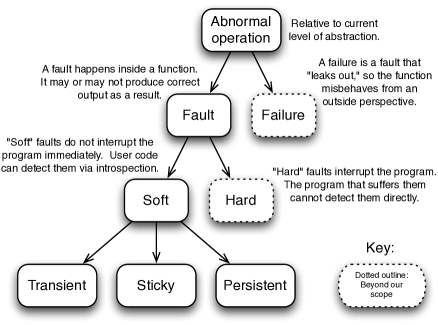
Figure 1: Classification of faults. Hard faults are outside the scope of our effort. We address soft faults in several ways.

The second characterization applies only to soft faults, and describes their temporal behavior:

• Persistent fault: The incorrect bit pattern will not change as execution proceeds. Example: The primary source of a data value (and any subsequent copies) are incorrect, so there is no ability to restore correct state.

• Sticky fault: The incorrect bit pattern can be corrected by direct action. Example: A backup source for the data exists and can be used to restore correct state.

• Transient fault: The incorrect pattern occurs temporarily. Example: Data in a cache is incorrect, but the correct value is still present in main memory and the cache value is flushed.

Figure 1 illustrates the relationship between the two characterizations of faults.

3.1 Potential for Soft Fault Detection and Correction

Although recovering from hard faults requires a coordinated effort across software and hardware layers, at least some soft faults can be effectively detected and corrected by user code. Furthermore, practically speaking, some applications spend much of their computation time in a small portion of the total program lines of code. Such applications can benefit from introducing fault-oriented introspection into that portion of the software. This situation occurs frequently in applications that generate and solve large linear systems of equations. In many cases, 80% or more of the computation time is spent in the linear solver. As problem sizes and processor counts increase, the solver can take more than 99% of the total execution time [28]. If we can incorporate introspection into the solvers for these cases, we can dramatically reduce the impact of soft faults.

One of the challenges for future system designers is determining how much fault resilience should be designed into the system. Historically, hardware and system architects have been very aggressive in capturing faults, so much so that users rarely experience a fault during normal system use. In the future, such approaches may be too expensive, resulting in a default reliability that must always be scrutinized. With this in mind, we introduce the concept of high vs. bulk reliability:

• Bulk reliability: The default reliability exhibited by system in normal execution mode. As system feature sizes shrink and component counts increase, we expect that bulk reliability will decrease to the point where users will need to pay attention to potential errors.

• High reliability: A special, presumably software-enabled mode, such that the user can declare data storage regions, data paths and execution regions that have better than bulk reliability.

Presently most algorithms lack robustness in the presence of soft faults. A single soft fault will not be detected and will eventually result in catastrophic failure. Assuming we have high reliability mechanisms in future programming environments, we have new opportunities for redesigning algorithms. Specifically, we seek algorithm designs such that decay in progress is proportional to the number of soft faults, at least in practice.

In this paper we focus on preconditioned iterative methods, and particularly on variants of GMRES (the Generalized Minimal Residual method [37]). We do so because, as we mentioned, many applications spend the vast majority of execution time in the solver, and GMRES is one of the most robust and popular methods for challenging problems. However, the approach we use is applicable to many algorithms. In fact, we believe that most, and maybe all, algorithms can eventually have fault-resilient formulations that introduce a very small runtime overhead while practically achieving the convergence equivalent to doing all computations in high reliability mode.

4 Models of reliability

In this section, we describe models of reliability that fault-tolerant numerical algorithms could use. The main goal of these models is to help algorithm developers reason about the quality of the computed solution. Without the promise of reliability for selected data and computations, no implementation of an algorithm can promise anything about the final result. Thus, all the models we propose in this section allow programmers to demand reliability as needed, and to allow data and control to flow between reliable and unreliable parts of the program.

A second goal of our reliability models is to convert hard faults into soft faults whenever our algorithms can handle the latter effectively. Reliability models govern the distinction between hard and soft faults. For example, the fail-stop model ensures that either the data and computations are reliable, or the program terminates with minimal side effects; it tries to turn all soft faults into hard faults. Current numerical algorithms assume a fail-stop model, which we assert can be relaxed in many cases. As long as algorithms can deal with soft faults without a large time-to-solution penalty, reducing the number of hard faults will improve performance by avoiding restarts and allowing reduction of the checkpoint frequency. It may even improve reliability, for example by avoiding the catastrophic situation of a second hard fault during recovery from one hard fault.

We begin in Section 4.1 by asking whether statistics could help us avoid considering models of reliability, and showing that it does not. Section 4.2 describes the “sandbox” model, which is the most general reliability model our fault-tolerant algorithms can use. The algorithm presented in Section 6 can work even in this model, but finer-grained models will allow us to define its convergence behavior more precisely. Therefore, we conclude with some desired features of finer-grained models in Section 4.3.

4.1 Statistical “model”

Increasingly numerical simulations use statistical techniques to account for uncertainty in the data as well as in the mathematical model. Many people refer to the study of representing and quantifying such uncertainties as uncertainty quantification (UQ). It seems reasonable that we also could apply these techniques to account for possibly unreliable solves, that is, “roll up” the solver’s uncertainty in that of the application itself. This would not require new solver algorithms or implementations. Instead, the problem would be solved multiple times using existing solvers, and statistics would be used to remove “outliers” and identify the most “believable” solution. This would comprise a “model” of reliability based on statistical belief, rather than on any guarantees made by the system or solver.

This “model” is no model of reliability at all. It implicitly assumes that faults may only occur in the solver, and that the statistical analysis that identifies the most believable solution is free of faults. In fact, these assumptions define the “sandbox” model of reliability described in the next section (4.2). Nevertheless, one might consider using statistical analysis to improve fault tolerance, in combination with a satisfactory fault model. We do not think this should be applied naïvely to existing fault-intolerant solvers, for two reasons. First, it may require running many solves to get statistical confidence. Second, it would throw away what numerical analysts have learned about how iterative solvers respond to certain kinds of faults. For example, perturbing the matrix $A$ affects convergence of iterative solvers more in earlier iterations than in later iterations (see Section 6.3). Finally, we will show in this paper that iterative methods can be modified to tolerate some soft faults, for much less cost than running a fault-intolerant solver many times. We do not dismiss statistical approaches completely, though. In particular, they may be useful to enhance detection of faults when invoking a solver. As we discuss in Section 7.3, our fault-tolerant inner-outer iteration can save some fault recovery work if it can detect faults reliably in the inner solves.

4.2 Sandbox model

Relaxing reliability of all data and computations may result in all manner of undesirable and unpredictable behavior. If instructions, pointers, array indices, and boolean values used for decisions may change arbitrarily at any time, we cannot assert anything about the results of a computation or the side effects of the program, even if it runs to completion without abnormal termination. The least we can do is force the fault-susceptible program to execute in a sandbox. This is a general idea from computer security, that allows the execution of untrusted “guest” code in a partition of the computer’s state (the “sandbox”) that protects the rest of the computer (the “host”) from the guest’s possibly bad behavior. Sandboxing can even protect the host against malicious code that aims to corrupt the system’s state, so it can certainly handle code subject to unintentional faults in data and instructions.

Sandboxes ensure isolation of a possibly unreliable phase of execution. They allow data to flow between reliable and unreliable phases of execution. Also, they let the host force guest code to stop within a predefined finite time, or if the host suspects the guest may have wandered astray. This feature is especially important in distributed-memory computation for preventing deadlock and other failures due to “crashed” or unresponsive nodes. In general, sandboxing converts some kinds of hard faults into soft faults, and limits the scope of soft faults to the guest subprogram.

Sandboxing may be implemented in different ways. For example, the guest may run in a virtual machine on the same hardware as the host. (See Smith and Nair [41] or Rosenblum [33] for accessible overviews of past and recent virtual machine technology.) Alternately, the guest may even run on separate hardware from the host program. For example, guests may run on a fast but unreliable subsystem, and the controlling host program may run on a reliable but slower subsystem.

Here is an example of the sandbox model in operation. In this example, the guest program is responsible for computing sparse matrix-vector products. It receives a vector $x$ from the host, computes $y:=A\cdot x$ (where $A$ is the sparse matrix), and returns $y$ to the host. The vectors $x$ and $y$ on the host are stored and computed with reliably. The guest makes no promises about the correctness of the values in the vector $y$ it returns. It may even return different values for the same $x$ input each time it is invokes. However, the sandbox ensures that the guest returns in finite time. (For example, it may kill the guest process if it takes too long, and return some arbitrary solution vector if the guest did not complete its computation.)

The fault-tolerant inner-outer iteration we will describe in Section 6 uses the sandbox model. There, the guest program performs the task “Solve a given linear system.” The host program invokes the guest repeatedly for different right-hand sides, and the host performs its own calculations reliably. See that section for details. Finer-grained models of reliability may improve accuracy of the inner solves, so we now go on to describe some desired features of these models.

4.3 Desired features of finer-grained models

The sandbox model of reliability makes only two promises of the unreliable guest: it returns something (which may not be correct), and it completes in fixed time. These already suffice to construct a working fault-tolerant iterative method, as we will show in Section 6. However, detecting faults or being able to limit how faults may occur would also be useful. All of these are more sophisticated forms of introspection. These finer-grained models of reliability can be used to improve accuracy of the iterative method, or to prove more specific promises about its convergence. We describe some of these below.

4.3.1 Detection

Knowing that no faults occurred in a bulk-reliability phase of execution can avoid robustness and recovery effort in the highly reliable phase. We discuss this more in Section 6 in the context of our inner-outer iteration. In general, if we know that the potentially unreliable inner solver experienced no faults, we know that its computed intermediate state (e.g., the Krylov subspace basis) is correct. We can then safely use that state to accelerate the next invocation of the inner solver. Fault detection is therefore a valuable feature of a reliability model, even without fault recovery. Many error-correcting storage schemes, such as those in DRAM memory, caches, and redundant disk storage, can detect more kinds of errors than those which they can correct. Extending those storage schemes to be able to correct those additional detectable errors requires additional hardware, energy consumption, and computation. Thus, if algorithms can exploit fault detection to handle faults efficiently, they can relieve hardware of the burden of recovery.

4.3.2 Transience

Faults should look as transient as possible. For example, consider solving the sparse linear system $Ax=b$ iteratively. If faults in the entries of $A$ persist throughout the iterative method, the method will be solving the wrong linear system $\tilde{A}x=b$. Worse yet, the algorithm will report that the computed approximate solution $\tilde{x}$ has a small residual norm $\|b-\tilde{A}\tilde{x}\|$, even though $\tilde{x}$ may be far from the actual solution. In contrast, many iterative methods naturally tolerate some kinds of occasional transient faults, so unreliable computations with only transient faults can still be useful. Indeed, before reliable electronic computers, the only “computers” were unreliable human beings. They could nevertheless solve real-world problems, because human faults are usually transient. (This is why, when balancing a checkbook by hand, it helps to repeat the process until one gets the same result more than once.)

Many hardware faults are not transient. This is particularly true of DRAM memory faults, as described for example in Schroeder et al. [38]. Permanent faults (which Schroeder et al. call “hard errors”) due to hardware failures are much more common than temporary faults. The so-called “chip-kill” DRAM error-correcting code (see Asanovic et al. [1]) was designed for the common case of an entire DRAM module failing permanently and producing incorrect values. In many cases, permanent faults interrupt a running program or even make the node fail, and are thus beyond the ability of an application to detect. That is, they are “hard faults” (see Section 3). However, applications may be able to detect and respond to these malfunctions as they first begin. Furthermore, “temporary” single-bit faults may persist and accumulate into multiple-bit faults, which some error-correcting codes cannot correct. Eliminating correctible faults before they become uncorrectible requires special measures (a “memory scrubber”) that may increase energy consumption and reduce available memory bandwidth.

This means the implementation of the reliability model likely will have to do extra work to give the appearance of transience. In terms of Section 3, the implementation must turn “persistent” faults into “sticky” or “transient” faults. For example, unreliable memory storing the sparse matrix $A$ could be refreshed every few iterations from a reliable backing store. Physical memory pages showing incorrect values during the refresh may be retired and replaced with other physical pages. The reliable backing store approach is also useful for checkpointing, and could be implemented with fast local storage (like flash memory).

4.3.3 Type system model

Consider implementing sparse matrix-vector multiply (the example of Section 4.2) as the guest program in the unreliable sandbox. If the guest can be arbitrarily unreliable, the sandbox has to do a lot of work to protect the host from things like invalid instructions (due to errors in instructions) or out-of-bounds array accesses (due to errors in index data). The sandbox could be much simpler if, for example, only the entries of the sparse matrix and vectors, and the floating-point computations with the matrix and vector values, are allowed to experience errors. This restriction would also make it easier for programmers to reason about what happens in code running inside the sandbox, so they would not need to write many redundant-looking checks that make code hard to read and maintain.

This example suggests a finer-grained programming model, in which developers can decide which data and computations they want to be reliable or unreliable, and mix the two in their program. For safety and ease of use, the default behavior of all data and computations should be as close to fail-stop reliability as possible. (That is, either the data and computations are reliable, or the program terminates.) Programmers may then relax reliability for certain data, or certain phases of computation, or both. In the above example, fail-stop default reliability ensures correctness of the sparse matrix indices and the sparse matrix-vector multiply routine, so the routine will not crash the entire program. This programming model is more demanding than the sandbox model, because it complicates the ways in which reliable and unreliable computations and data may interact.

We are currently exploring a special case of this model, in which programmers can allocate “unreliable memory” by calling a special version of C’s malloc routine. The operating system records and reports to the application any detected but uncorrectible memory faults in memory areas marked unreliable, but it does not kill the process that allocated this memory, as many operating systems do for ordinary memory allocations. We believe this programming interface - based approach will work for special cases of faults. However, we think the best way to generalize this reliability model for all kinds of faults in different hardware components would be to encode reliability in the type system of the programming language, much as existing type systems encode the precision of floating-point values or whether an object should be protected from simultaneous access by multiple threads. We do not require new programming language features for the numerical methods proposed in this paper, but we think it would make designing and implementing fault-tolerant algorithms much easier.

Encoding reliability in the type system is not a new idea. Chen et al. [13] observe that different data in different algorithms may need different levels of storage reliability, and that reliability costs energy, space, performance, or some combination of them. They propose programmer annotations for declaring reliability of subsets of multidimensional arrays. For the simple case of nested for loops over the arrays, they then use compiler analysis to derive what parts of the arrays should be stored reliably. Our suggested “reliability on demand” feature is also a kind of programmer annotation. However, it applies to entire data structures and computations, rather than subsets of arrays. Chen et al. require complicated compiler analysis of loops to derive the reliable regions of arrays and generate separate reliable and unreliable code. Our annotations would depend only on simple type declarations and compiler analysis, analogous to that already performed by compilers when combining values of different floating-point precisions.

4.3.4 Reliable parallel decisions

Parallel computing introduces new ways in which soft faults can turn into hard faults. For example, if the contents of messages between nodes of a distributed-memory computer may become corrupted, then different nodes may get different results in an all-reduce, even if each node computes its part of the all-reduce reliably. Many distributed-memory implementations of iterative methods use the result of an all-reduce in a predicate that tells the method when to stop iterating (for example, when the residual norm is less than some tolerance). The predicate is computed redundantly on each node, with the expectation that all nodes will get the same result. If they do not – for example, if they have different values for the residual norm – then some nodes may stop iterating while others continue. This can result in deadlock or application failure, that is, it can turn a soft fault into a hard fault. We would prefer that parallel decisions like this one be reliable.

This is not a new problem; Blackford et al. [8] discuss it in the less extreme context of heterogeneous clusters, where different processors may have different floating-point properties and thus may evaluate floating-point comparisons differently. They recommend in this case that one processor compute the stopping criterion and broadcast the Boolean result to all other processors. This would only solve the reliability problem for convergence tests if Boolean-valued messages cannot be corrupted or lost. In our case, it would be simpler, and probably no more costly, to require the original all-reduce and the predicate evaluation to be reliable and produce the same result on all nodes.

A different approach would be to observe that the stopping criterion is a special case of distributed agreement on a Boolean value. This is an instance of the thoroughly studied Byzantine Generals Problem (Lamport et al. [26]), for which practical solution algorithms exist (see e.g., Castro and Liskov [12]). This problem assumes that some of the entities participating in distributed agreement may intentionally attempt to deceive the others, which is an extreme but valid generalization of corrupted data and arithmetic on some processors. In practice, simple distributed agreement schemes should suffice. For example, an implementation could augment the all-reduce input for the convergence test with a simple integer variable which each processor would set to one if it has reached convergence. Then all processors would declare convergence if the sum of these integer values was greater than some portion of the total processors being used. Alternately, it may be simpler just to assume high reliability for all distributed-memory transactions. For example, practically speaking, the cost of an all-reduce is dominated by latency (or even just the fact that the message is transmitted off the node), so adding reliability by computing redundantly or by adding error detection and correction metadata to the all-reduce data package is almost free.

5 Desired properties of fault-tolerant iterations

Fault-tolerant iterative methods should have certain properties in order to be both useful and feasible to implement. In this section, we describe a few desired properties, and explain which make sense to implement. Section 5.1 introduces two desired convergence properties – eventual convergence and gradual degradation of convergence – and argues for eventual convergence as the most reasonable criterion. Section 5.2 discusses properties of implementations of these methods that will help them achieve good performance, with minimal changes to existing solver algorithms and implementations. These criteria will help us narrow the space of possible algorithms.

5.1 Convergence-related properties

We call what we see as the most important property eventual convergence: If a comparable but not fault-tolerant method would converge to the right answer in the case of no faults, the fault-tolerant solver should either converge to the right answer in a finite number of steps, or tell the caller that it did not. The fault-tolerant method may require more iterations or otherwise take more time, and it might also have an upper bound on the number or magnitude of faults it can tolerate. One iterative method that does not have the eventual convergence property is iterative refinement (an algorithm first described by Wilkinson [45]). Given sufficiently large faults, only one fault in the residual vector need happen at the “last iteration” for iterative refinement never to compute the right answer. Without eventual convergence, it would not be worthwhile to relax hardware reliability, since all the effort at previous iterations might be wasted by a single fault. It is often impossible to know when an fault will occur in a particular component, so a reasonable method should allow them to occur at any time. The algorithm we present in Section 6 does have the eventual convergence property.

Gradual degradation of convergence as the number of faults increases would also be desirable. This might be much harder to guarantee than eventual convergence. For example, consider an explicit Petrov-Galerkin projection method for solving the $n\times n$ system $Ax=b$, that adds basis vectors to two different bases $V_{k}=[v_{1},\dots,v_{k}]$ and $W_{k}=[w_{1},\dots,w_{k}]$. Implementing a method mathematically equivalent to GMRES, for instance, would require $\mathcal{R}\left(V_{k}\right)$ $=$ $\operatorname{span}\{r_{0}$, $Ar_{0}$, $\dots$, $A^{k-1}$ $r_{0}\}$ and $\mathcal{R}\left(W_{k}\right)=A\mathcal{R}\left(V_{k}\right)$. If the matrix-vector products were unreliable, we could still extend the basis in every iteration by adding a random basis vector and orthogonalizing it against the previous basis vectors, if the basis vectors are computed reliably. In the worst case, this unreliable method would not converge until $\mathcal{R}\left(W_{k}\right)$ spans the entire space, that is, on iteration $n-1$. In fact, GMRES cannot promise better than this even in the case of no faults. It is possible to construct $n\times n$ problems for which the residual in ordinary GMRES does not decrease until iteration $n-1$, or for which the residual exhibits any desired nonincreasing convergence curve [18]. Some real-life linear systems exhibit almost no convergence until some number of iterations, after which they converge rapidly. This suggests that eventual convergence is a more reasonable goal than gradual degradation of convergence. We will show in the numerical experiments in Section 8 that our FT-GMRES algorithm exhibits gradual degradation of convergence in practice. It may do so in theory also, though we do not attempt in this paper to prove this.

5.2 Implementation-related properties

We have already discussed different models of application-controlled reliability in Section 4. Making all data and arithmetic reliable would trivially result in a fault-tolerant iterative method. However, all of our models assume that reliability has a cost, which is some combination of additional energy or storage and reduced performance. Thus, a fault-tolerant algorithm should aim to store most of its data and spend most of its computations in unreliable mode. Second, fault-tolerant algorithms should not be too much slower than corresponding less tolerant algorithms. It is reasonable to expect that the longer an application runs, the more faults it will likely encounter. More faults mean either slower convergence, which compounds the problem, or even solver failure. If the fault-tolerant method is too slow, it may be faster just to run a less tolerant method over and over using an ensemble approach until the majority of answers agree. Finally, fault-tolerant methods should reuse existing algorithms and implementations as much as possible. In particular, they should accept existing preconditioner algorithms, and ideally even existing implementations. Preconditioners are often complicated and specific to their application. Our inner-outer iteration in Section 6 can call existing iterative solvers and their preconditioners as a “black box,” as long as they promise to terminate within a fixed time.

6 Fault-Tolerant GMRES

This section describes the Fault-Tolerant GMRES (FT-GMRES) algorithm, a Krylov subspace method for iterative solution of large sparse linear systems $Ax=b$. FT-GMRES computes the correct solution $x$ even if the system experiences uncorrected faults in both data and arithmetic [21]. It promises “eventual convergence” in the sense of Section 5.1: it will always either converge to the right answer, or (in rare cases) stop and report immediately to the caller if it cannot make progress. FT-GMRES accomplishes this by dividing its computations into reliable and unreliable phases, using the sandbox model of reliability described in Section 4.2. Rather than rolling back any faults that occur in unreliable phases, as a checkpoint / restart approach would do, FT-GMRES “rolls forward” through any faults in unreliable phases, and uses the reliable phases to drive convergence. FT-GMRES can also exploit fault detection in order to correct corrupted data during unreliable phases.

6.1 FT-GMRES is based on Flexible GMRES

Algorithm 1 (Right-preconditioned) GMRES

1:Linear system $Ax=b$ and initial guess $x_{0}$

2:Approximate solution $x_{m}$ for some $m\geq 0$

3:

4:$r_{0}:=b-Ax_{0}$$\triangleright$ Unpreconditioned initial residual vector

5:

6:$\beta:=\|r_{0}\|_{2}$

7:

8:$q_{1}:=r_{0}/\beta$

9:

10:for $j=1,2,\dots$ until convergence do

11:

12:Solve $q_{j}=Mz_{j}$ for $z_{j}$$\triangleright$ Apply preconditioner

13:

14:$v_{j+1}:=Az_{j}$$\triangleright$ Apply the matrix $A$

15:

16:for $i=1,2,\dots,k$ do$\triangleright$ Orthogonalize

17:

18:$H(i,j):=q_{i}^{*}v_{j+1}$

19:

20:$v_{j+1}:=v_{j+1}-q_{i}H(i,j)$

21:end for

22:

23:$H(j+1,j):=\|v_{j+1}\|_{2}$

24:

25:$q_{j+1}:=v_{j+1}/H(j+1,j)$$\triangleright$ New basis vector

26:

27:$y_{j}:=\operatorname{argmin}_{y}\|H(1:j+1,1:j)y-\beta e_{1}\|_{2}$

28:

29:$x_{j}:=x_{0}+M^{-1}[q_{1},q_{2},\dots,q_{j}]y_{j}$$\triangleright$ Compute solution update

30:end for

Algorithm 2 Flexible GMRES (FGMRES)

1:Linear system $Ax=b$ and initial guess $x_{0}$

2:Approximate solution $x_{m}$ for some $m\geq 0$

3:

4:$r_{0}:=b-Ax_{0}$$\triangleright$ Unpreconditioned initial residual

5:

6:$\beta:=\|r_{0}\|_{2}$

7:

8:$q_{1}:=r_{0}/\beta$

9:

10:for $j=1,2,\dots$ until convergence do

11:

12:Solve $q_{j}=M_{j}z_{j}$$\triangleright$ Apply current preconditioner

13:

14:$v_{j+1}:=Az_{j}$$\triangleright$ Apply the matrix $A$

15:

16:for $i=1,2,\dots,k$ do$\triangleright$ Orthogonalize

17:

18:$H(i,j):=q_{i}^{*}v_{j+1}$

19:

20:$v_{j+1}:=v_{j+1}-q_{i}H(i,j)$

21:end for

22:

23:$H(j+1,j):=\|v_{j+1}\|_{2}$

24:

25:Update rank-revealing decomposition of $H({1}\nobreak\mskip 1.0mu\mathpunct{}\nonscript\mkern-3.0mu{:}\mskip 1.0mu{}{j},{1}\nobreak\mskip 1.0mu\mathpunct{}\nonscript\mkern-3.0mu{:}\mskip 1.0mu{}{j})$

26:

27:if $H(j+1,j)$ is less than some tolerance then

28:

29:if $H({1}\nobreak\mskip 1.0mu\mathpunct{}\nonscript\mkern-3.0mu{:}\mskip 1.0mu{}{j},{1}\nobreak\mskip 1.0mu\mathpunct{}\nonscript\mkern-3.0mu{:}\mskip 1.0mu{}{j})$ not full rank then

30:

31:Did not converge; report error

32:

33:else

34:

35:Return at end of this iteration$\triangleright$ Discovered invariant subspace

36:end if

37:

38:else

39:

40:$q_{j+1}:=v_{j+1}/H(j+1,j)$

41:end if

42:

43:$y_{j}:=\operatorname{argmin}_{y}\|H({1}\nobreak\mskip 1.0mu\mathpunct{}\nonscript\mkern-3.0mu{:}\mskip 1.0mu{}{j+1},{1}\nobreak\mskip 1.0mu\mathpunct{}\nonscript\mkern-3.0mu{:}\mskip 1.0mu{}{j})y-\beta e_{1}\|_{2}$

44:

45:$x_{j}:=x_{0}+[z_{1},z_{2},\dots,z_{j}]y_{j}$$\triangleright$ Compute solution update

46:end for

FT-GMRES is based on Flexible GMRES (FGMRES) [34], shown here as Algorithm 2. FGMRES extends the Generalized Minimal Residual (GMRES) method of Saad and Schultz [37], by “flexibly” allowing the preconditioner to change in every iteration. We show standard right-preconditioned GMRES as Algorithm 1 for comparison. An important motivation of flexible methods are “inner-outer iterations,” which use an iterative method itself as the preconditioner. In this case, “solve $q_{j}:=M_{j}z_{j}$” (Line 12 of Algorithm 2) means “solve the linear system $Az_{j}=q_{j}$ approximately using a given iterative method.” This inner solve step preconditions the outer solve (in this case the FGMRES flexible iteration). Changing right-hand sides and possibly changing stopping criteria for each inner solve mean that if one could express the “inner solve operator” as a matrix, it would be different on each invocation. This is why inner-outer iterations require a flexible outer solver.

Flexible methods need not use an iterative method for the inner solves. The $M_{j}$ may be arbitrary functions from the range of $A$ to the domain of $A$. Most importantly, the preconditioners may change significantly from one iteration to another; flexible methods do not depend on the difference between successive preconditioners being small. This is the key observation behind FT-GMRES: flexible iterations allow successive inner solves to differ arbitrarily, even unboundedly. This suggests modeling faulty inner solves as “different preconditioners.” Taking this suggestion leads to FT-GMRES, which we present in the next section.

Flexible inner-outer iterations have the property that the dimension of the Krylov subspace from which they choose the current approximate solution grows at each outer iteration [39], as long as the break-down condition mentioned above does not occur. This ensures eventual convergence. Corresponding restarted Krylov methods lack this property; their convergence may stagnate. Even though this property of inner-outer iterations may not hold in the case of faulty inner solves, the numerical experiments in Section 8 show that inner-outer iterations offer better fault tolerance than simply restarting. Both restarting and inner-outer iterations correspond naturally to the sandbox reliability model when the number of iterations per restart cycle resp. inner solve is fixed.

There are flexible versions of other iterative methods besides GMRES, such as CG [17] and QMR [43], which could also be used as the outer solver. We chose FGMRES because it is easy to implement, robust, and can handle nonsymmetric linear systems. Experimenting with other flexible outer iterations is future work.

6.1.1 Flexible GMRES’ additional failure mode

FGMRES has an additional failure mode beyond those of standard GMRES. The quantity $H(j+1,j)=0$ does not necessarily indicate convergence, as it would in standard GMRES. This is because $H({1}\nobreak\mskip 1.0mu\mathpunct{}\nonscript\mkern-3.0mu{:}\mskip 1.0mu{}{j},{1}\nobreak\mskip 1.0mu\mathpunct{}\nonscript\mkern-3.0mu{:}\mskip 1.0mu{}{j})$ is always nonsingular in GMRES if $j$ is the smallest iteration index for which $H(j+1,j)=0$, whereas $H({1}\nobreak\mskip 1.0mu\mathpunct{}\nonscript\mkern-3.0mu{:}\mskip 1.0mu{}{j},{1}\nobreak\mskip 1.0mu\mathpunct{}\nonscript\mkern-3.0mu{:}\mskip 1.0mu{}{j})$ may not be nonsingular in FGMRES in that case. (This is Saad’s Proposition 2.2 [34].) This can happen even in exact arithmetic. For example, it may occur due to unlucky choices of the preconditioners: for example, $M_{j}^{-1}=A$ and $M_{j+1}^{-1}=A^{-1}$. In practice, this case is rare, even when inner solves are subject to faults. Furthermore, it can be detected inexpensively, since there are algorithms for updating a rank-revealing decomposition of an $m\times m$ matrix in $O(m^{2})$ time (see e.g., Stewart [42]). This is no more time than it takes to update the QR factorization of the upper Hessenberg matrix at iteration $m$. The ability to detect this rank deficiency ensures “trichotomy” of FGMRES: it either

1. converges to the desired tolerance,

2. correctly detects an invariant subspace, with a clear indication ($H(j+1,j)=0$ and $H({1}\nobreak\mskip 1.0mu\mathpunct{}\nonscript\mkern-3.0mu{:}\mskip 1.0mu{}{j},{1}\nobreak\mskip 1.0mu\mathpunct{}\nonscript\mkern-3.0mu{:}\mskip 1.0mu{}{j})$ is nonsingular), or

3. gives a clear indication of failure ($H(j+1,j)\neq 0$ and detected rank deficiency of $H({1}\nobreak\mskip 1.0mu\mathpunct{}\nonscript\mkern-3.0mu{:}\mskip 1.0mu{}{j},{1}\nobreak\mskip 1.0mu\mathpunct{}\nonscript\mkern-3.0mu{:}\mskip 1.0mu{}{j})$).

We base FT-GMRES’ “eventual convergence” on this trichotomy property. In the following section, we will discuss recovery strategies that FT-GMRES can use in case of the third condition above.

6.2 Fault-Tolerant GMRES

FGMRES’ acceptance of significantly different preconditioners at each iteration suggests modeling solver faults as “different preconditioners.” The least disruptive approach for existing solvers is to use the inner-outer iteration approach. The outer FGMRES iteration wraps any existing solver, which is used as the inner iteration. Any solver works, even a sparse direct method (in which case the inner “iteration” is not actually an iterative method), an iterative method with any or no preconditioner, or a specialized algorithm that exploits problem structure (such as an FFT or hierarchical matrix factorization). Existing preconditioners may also be used without algorithmic modifications. We call the resulting inner-outer iteration Fault-Tolerant GMRES. It is shown here as Algorithm 3. Inner-outer iterations with FGMRES have been used as a kind of iterative refinement in mixed-precision computation (see Buttari et al. [11]), but as far as we know, this is the first time it has been used for reliability and robustness against possibly unbounded errors.

Algorithm 3 Fault-Tolerant GMRES (FT-GMRES)

1:Linear system $Ax=b$ and initial guess $x_{0}$

2:Approximate solution $x_{m}$ for some $m\geq 0$

3:

4:$r_{0}:=b-Ax_{0}$

5:

6:$\beta:=\|r_{0}\|_{2}$

7:

8:$q_{1}:=r_{0}/\beta$$\triangleright$ Unpreconditioned initial residual vector

9:

10:for $j=1,2,\dots$ until convergence do

11:

12:Inner solve (unreliable) for $z_{j}$ in $q_{j}=Az_{j}$

13:

14:$v_{j+1}:=Az_{j}$$\triangleright$ Apply the matrix $A$

15:

16:for $i=1,2,\dots,k$ do$\triangleright$ Orthogonalize

17:

18:$H(i,j):=q_{i}^{*}v_{j+1}$

19:

20:$v_{j+1}:=v_{j+1}-q_{i}H(i,j)$

21:end for

22:

23:$H(j+1,j):=\|v_{j+1}\|_{2}$

24:

25:Update rank-revealing decomposition of $H({1}\nobreak\mskip 1.0mu\mathpunct{}\nonscript\mkern-3.0mu{:}\mskip 1.0mu{}{j},{1}\nobreak\mskip 1.0mu\mathpunct{}\nonscript\mkern-3.0mu{:}\mskip 1.0mu{}{j})$

26:

27:if $H(j+1,j)$ is less than some tolerance then

28:

29:if $H({1}\nobreak\mskip 1.0mu\mathpunct{}\nonscript\mkern-3.0mu{:}\mskip 1.0mu{}{j},{1}\nobreak\mskip 1.0mu\mathpunct{}\nonscript\mkern-3.0mu{:}\mskip 1.0mu{}{j})$ not full rank then

30:

31:Try recovery strategies discussed in text

32:

33:else

34:

35:Return at end of this iteration$\triangleright$ Discovered invariant subspace

36:end if

37:

38:else

39:

40:$q_{j+1}:=v_{j+1}/H(j+1,j)$

41:end if

42:

43:$y_{j}:=\operatorname{argmin}_{y}\|H({1}\nobreak\mskip 1.0mu\mathpunct{}\nonscript\mkern-3.0mu{:}\mskip 1.0mu{}{j+1},{1}\nobreak\mskip 1.0mu\mathpunct{}\nonscript\mkern-3.0mu{:}\mskip 1.0mu{}{j})y-\beta e_{1}\|_{2}$

44:

45:$x_{j}:=x_{0}+[z_{1},z_{2},\dots,z_{j}]y_{j}$$\triangleright$ Compute solution update

46:end for

The only part of FT-GMRES allowed to run unreliably is Line 12, which invokes the inner solver. FT-GMRES expects that inner solves do most of the work, so inner solves run in the less expensive unreliable mode. Inner solvers need only return with a solution in finite time (see Section 4.2). That solution may be completely wrong if errors occurrred. Within the inner solves, the matrix $A$, right-hand side $b$, and any other inner solver data may change arbitrarily, and those changes need not even be transient. However, each outer iteration of FT-GMRES must run reliably, and requires a correct version of the matrix $A$, right-hand side $b$, and additional outer solve data (the same that FGMRES would use).

Since FT-GMRES expects only a small number of outer iterations, interspersed by longer-running inner solves, we need not store two copies (unreliable and reliable) of $A$ and $b$ in memory. Instead, we can save them to a reliable backing store, or even recompute them. If the system provides fault detection capability, we can avoid recovering or recomputing these data if no faults occurred, or even selectively recover or recompute just the corrupted parts of the critical data. If the inner solve itself knows that no errors occurred, it could also aggressively continue improving the solution before returning to the outer iteration; we leave this option for future work.

One practical point is that the outer iteration must scan the result of each inner solve for invalid floating-point values (NaN and Inf), and replace any with valid values. The latter need not be correct – for example, they may be random numbers, or (better) averages of their neighbors with respect to the matrix structure. Many iterative methods perform this scan already for incomplete factorization preconditioning, since there often is no way to know in advance that the incomplete factors are nonsingular.

Line 31 of Algorithm 3 covers the case where the outer iteration appears to have converged, but the current upper Hessenberg matrix is rank deficient. This can happen in FGMRES as well, even with no faults. There, it indicates an unlucky combination of preconditioner applications. In the case of FT-GMRES, that unlucky combination may have occurred due to faults. One of the following recovery strategies may be appropriate:

1. retry the current iteration starting from Line 12 inclusive;

2. retry the current iteration after Line 12, but replace $z_{j}$ with a random vector (scaled appropriately according to best estimates of $\|A^{-1}\|$); or

3. stop and return $x_{j-1}$, the last good approximate solution.

In parallel, all these strategies require agreement between processors, and therefore global communication. However, the processors have to agree anyway whether to continue iterating based on the convergence criterion, so no additional communication is needed. In our numerical experiments discussed in Section 8, we found the rank-deficient upper Hessenberg case to be rare.

Another feature of the inner-outer iteration approach is that we can reuse information from previous inner iterations, if we know somehow that they were error-free. For example, we could use a Krylov basis recycling technique and restart, or simply keep the previous iteration’s data and continue without restarting (for an (F)GMRES inner iteration). Thus, the implementation can use whatever information about errors is available, though it does not require this information.

6.3 Inexact Krylov as an analysis tool

Inexact Krylov methods allow solving $Ax=b$ by using successive approximations $A_{k}$ of $A$. This makes them a generalization of flexible methods, since the matrix, as well as the preconditioner, may change in every iteration. For overviews and development of convergence theory, see Simonici and Szyld [40] and van den Eshof and Sleijpen [44]. These methods convergence when the error between the actual matrix $A$ and each approximation $A_{k}$ respects a varying bound. The bound starts small, but grows inversely as a function of the current residual norm. Inexact Krylov methods are motivated by applications where computing $A$ itself is prohibitively expensive, but computing $w=Av$ for a vector $v$ can be done approximately, and more effort in the approximation results in less error.

Inexact Krylov methods cannot be used to provide tolerance against arbitrary data and computational faults when applying the matrix $A$. This is because they require an error bound which is usually not as large as many possible bit flips. (Bit flips may occur in exponent bits as well as sign and significand bits.) Furthermore, if a fault in applying $A$ results in an error which is larger than the current bound, inexact Krylov methods cannot promise convergence. Nevertheless, inexact Krylov offers a framework for analyzing FGMRES convergence. If a reliability model lets us control and bound inner solves’ errors, we can use this framework.

Inexact Krylov methods also give insight into where to focus reliability efforts. For example, convergence of inexact GMRES depends more on orthogonality of the basis vectors than convergence of standard GMRES [40]. This suggests spending more effort on basis vector reliability than on reliability of the matrix and preconditioner. Furthermore, the inexact Krylov framework suggests that the matrix $A$ and preconditioner(s) should be applied more reliably in initial iterations, if possible. This coincides with our informal experimental observation that perturbing the matrix $A$ affects convergence of iterative solvers more in earlier iterations than in later iterations.

7 Programming model details

When we presented the FT-GMRES algorithm in Section 6, we declared few assumptions about the reliability programming model. The algorithm needs few; the “sandbox” model (Section 4.2) suffices for correctness, and maps naturally to inner-outer iterations in general. However, existing computer systems require few modifications to offer a richer model, which can also help us implement FT-GMRES more efficiently. In this section, we describe a programming model that is both suited for FT-GMRES, and is reasonable for systems architects to implement. This model promises reliable data and computations within the specified time and space bounds, and provides best-effort fault detection outside those bounds. It includes schemes for efficient local recovery of possibly corrupted data. We were able to implement a representative subset of this model for our performance prototype (Section 11) with reasonable effort.

In Section 7.1, we show how the data in FT-GMRES and analogous methods naturally separate into categories based on required reliability, and the amount of time and memory it consumes. Section 7.2 explains why we assume only best-effort fault detection, though better fault detection guarantees could improve performance. In Section 7.3, we describe how the FT-GMRES algorithm itself, plus best-effort fault detection, lead to a two-stage recovery scheme for corrupted data. This scheme makes approximate repairs in inner iterations, and performs preferably local full recovery of corrupted data in outer iterations.

Throughout this section, we refer to the subset of the model we implemented for the performance experiments discussed in Section 11. This system currently only handles detected but uncorrectible DRAM memory faults, not other kinds of faults such as incorrect arithmetic or corrupted MPI messages. This restriction was convenient for developing a prototype in reasonable time. We argue in Section 7.5 that a system that considers only memory faults nevertheless includes the right programming model elements for developing algorithms that can handle all kinds of faults. Finally, Section 7.6 proposes that our model is sufficiently general that it could work for other numerical methods based on subspace search and fixed-point iteration.

7.1 Which data reliable, when

In this section, we explain which data in our fault-tolerant iterative method we allow to experience faults, and when in the algorithm we allow those faults to occur. In particular, we allow faults in all “large” data and computations in the inner iterations only. “Large” data includes sparse matrices, preconditioners, and vectors, but does not include the small projected linear system or least-squares problem used to compute the solution update coefficients, nor does it include code or control data such as loop indices. We also explain which of the large data require occasional recovery to their original uncorrupted state. Finally, we argue that this programming model could apply to other Krylov subspace methods, and to subspace search and fixed-point iterations in general.

7.1.1 “Large” and “small” data

Krylov methods for solving linear systems spend most of their memory and time computing with two kinds of objects: “large” dense vectors, and linear operators (functions from a vector to a vector) of the same dimension(s). The latter include sparse matrices (where the function is sparse matrix-vector multiplication), linear operators implemented as a subroutine (e.g., by discretizing and solving a partial differential equation) rather than as a sparse matrix, and preconditioners (if applicable).

Krylov methods project a larger linear system onto a smaller linear system or least-squares problem which is inexpensive to solve using either dense factorizations, or an equivalent small number of scalar computations. This gives us a subjective but practical definition of “large” data: using a Krylov method to solve a linear system of that size saves time, memory, or both, relative to a dense factorization. Krylov methods also include “small” data: scalars or small dense matrices and vectors which represent the projected linear system or least-squares problem. The projected problem is used to solve for the coefficients of the solution update. The projected problem requires little memory or solution time computed with the large vectors and operators. Its small size makes it sensitive to corrupted data or computations, yet the resulting solution update coefficients have a large effect on the accuracy of the computed solution vector. Thus, we require that the projected problem be stored and computed reliably, and confine any unreliable data or computation to the large vectors and operators.

7.1.2 Both operators and vectors may be unreliable

The large matrix $A$ and preconditioner(s) typically take up much more memory than a single vector or corresponding size. Also, applying the matrix or a preconditioner to a vector takes more time than computing a single vector operation (such as a norm, inner product, or vector sum). However, the balance of time and memory between operator applications and vector operations varies between Krylov methods. For example, our inner solver uses GMRES (the Generalized Minimal Residual method [37]), which may spend more of its time in vector operations, depending on the restart length. Thus, we allow vectors as well as operators in the inner solver to be unreliable, since otherwise the solver might require too much unreliable data and computation. The goal is for a fault-tolerant solver to spend most of its time and memory in unreliable mode.

7.2 Best-effort fault detection

We pessimistically assume best-effort fault detection. This means that a significant fraction of faults might evade detection. We assume this in part due to technical limitations of our software prototype. Currently, it can only detect injected faults by simulating an ECC memory “patrol scrubber” in software, using a separate, asynchronously executing thread. Injected faults encountered by user code’s actual memory operations are not detected. This is because the current version of Linux, on which our software prototype depends, kills any user process whose memory operations encounter an uncorrectable fault. (It need not do this for faults detected by an actual patrol scrubber.) Changing this behavior would require a custom Linux patch, which in turn would prohibit us from running tests on computers we do not administer. Many other operating systems have this property.

Despite this technical limitation of our prototype, we believe that our pessimistic assumption is reasonable in production systems. For example, most current systems offer no hardware detection of arithmetic faults. Without expensive hardware replication, the best a system could do is insert occasional test instructions into the instruction stream. This would be mostly likely to detect “sticky” arithmetic faults, but not transient ones. Detection might also be asynchronous, so that faults contaminate other computations irreversibly before the system detects and reports them to the application. For instance, a hardware ECC memory patrol scrubber might discover uncorrectable corruption in a sparse matrix entry while the Krylov method is doing something else. Future systems may not necessarily promise anything about the delivery time of the resulting error report. Finally, fault detection does cost energy and / or performance. Our algorithm does not require infallible fault detection for correctness, so we are willing to relax this, as long as system architects can meet our reliability demands.

7.3 Repair of corrupted data

7.3.1 How Krylov methods use operators

Krylov methods for solving linear systems use “large” linear operators in two different ways. The first way is iterative: the method repeatedly applies the operator(s) to a vector, in order to build up one or more search spaces. The theory of inexact Krylov methods says that the operators need not be applied exactly at all iterations in order for the method to converge. We take this as inspiration for allowing these operator applications to vary arbitrary, due to unreliability. The second way is for computing the residual vector of the current approximate solution explicitly. The residual vector may then be used to verify the approximate solution, restart the iteration, or improve the solution in an outer iteration. These uses of the residual vector require an exact computation, not an approximation, using just the matrix $A$ and right-hand side $b$. Techniques like iterative refinement even require computing the residual vector in higher precision, in order for certain convergence results to hold.

Constructing the operators always happens outside of the Krylov method. Construction may be a complicated operation consuming a significant part of the application’s total run time, and many more lines of code than the linear solver. (Consider a structural dynamics application using the finite element method, for example.) It is usually a nonlocal operation as well: that is, it requires communication when running in parallel in a distributed-memory environment. (For example, in the finite element method, assembling elements with mesh points owned by different processors requires summing contributions from the involved processors.) However, the operators usually do not change or need expensive reconstruction during the Krylov method.

Note that solving linear systems with a Krylov method often requires an effective preconditioner. Preconditioners can be time-consuming to compute, and this computation often requires global communication. Algebraic multigrid is a good example. The only difference between a preconditioner and the matrix $A$ is that for GMRES variants, a left preconditioner is not needed in order to compute a residual vector. Many GMRES users prefer a right preconditioner anyway, since it ensures that the projected least-squares problem’s solution has the same residual norm as the approximate solution, in exact arithmetic. GMRES requires the right preconditioner in order to compute the approximate solution or current residual vector; thus, computing these vectors reliably requires applying the right preconditioner reliably.

7.3.2 What this says about operator recovery

The above two paragraphs say that (a) a fault-tolerant Krylov method must be able to apply operators both reliably and unreliably, and (b) constructing an operator is expensive and nonlocal. This suggests that a fault-tolerant Krylov method must be able to recover the original operators reliably, and that this recovery should not require recomputing the affected operator. We suggest implementing this using a local checkpointing scheme, which saves matrix and preconditioner data that may experience memory faults to reliable backing storage. We already assume that FT-GMRES marks this data as unreliable, and that FT-GMRES notifies the system on entry to each inner iteration that faults are allowed. The checkpointing mechanism need only pay attention to these notifications to decide when and what to checkpoint. The reliable backing store should be fast, nonvolatile, and local to each node. Recent projections for exascale-class systems predict much heavier use of node-local scratch storage (see e.g., [25, Section 5.6.3.1]). We expect, therefore, that future supercomputers will include node-local solid-state drives, meant for scratch storage or as a cache for input / output operations. We currently lack access to such hardware, so as a proxy, we implemented for this paper a reliable backing store using ordinary DRAM memory in which we do not allow detected but uncorrectible ECC faults (see Section 11).

7.3.3 Krylov basis vectors

We did not mention the Krylov basis vectors computed by the inner iteration in the paragraphs above. These vectors result from applying a possibly corrupted matrix or preconditioner; they are “corrupted by construction.” Thus, it does not make sense to save or restore them. Vectors computed by the outer iteration should be completely reliable, however. Corruption of Krylov basis vectors in the outer iteration may result in an incorrect solution.

7.3.4 Local and approximate recovery

Local recovery is important. Faults like bit flips in memory and incorrect arithmetic are local to the node (or even to the CPU). Recomputation of an operator typically involves global communication, whose pattern of dependencies typically make it a heavyweight global synchronization point. As supercomputers grow towards exascale, the increasing cost of communication makes favoring local operations more and more attractive. The checkpointing scheme mentioned above offers an exact local recovery method. If the system offers reliable detection of data corruption, including fault locations, approximate local repair is possible. As we explain in Section 11, existing ECC memory hardware provides this information to the operating system upon encountering an uncorrectible error. The application can then define a handler that repairs the fault. For example, a corrupted sparse matrix entry can be “smoothed out” by replacing it with the average of its neighbors. Simple handlers cost little more than the system interrupt caused by the fault itself.

Approximate repair is an inexpensive option for inner iterations. However, outer iterations require exact recovery of operators. Since corrupted data locations are unknown in advance, restoring the operators requires either full local checkpointing, or global recomputation. This suggests a two-fold recovery strategy. Start each inner iteration with the correct sparse matrix and preconditioner(s), but allow data corruption to occur. If possible, try to fix corrupted values during the inner iteration, but do so only locally, and as quickly as possible, even if that means the values are only recovered approximately. Quick fixes minimize the idle time of other processors which did not experience data corruption. Local fixing avoids communication overhead in the performance-critical inner iteration. At the end of the inner iteration, refresh the correct values in the sparse matrix, even if no faults were detected there. This ensures correctness even if undetected faults occurred. Perform the outer iteration, and continue. Since we expect outer iterations to occur infrequently, we can afford to spend more there on recovery than in inner iterations.

7.4 Summary of model

The above discussion implies three tiers of data and computation:

1. Always reliable data, such as the projected linear system, code, and control data (e.g., loop indices).

2. Data which may be unreliable in inner phases, must be reliable in outer phases, and which the outer iteration must be able to refresh to correct values. Examples: the matrix, preconditioner(s), and right-hand side of the linear system $Ax=b$ to solve.

3. Unreliable data which does not require saving or restoring, such as the Krylov basis vectors in inner iterations.

7.5 Memory faults are sufficient

The performance prototype of FT-GMRES we describe in this work was designed to handle faults in DRAM memory. Computer hardware may also experience corrupted caches or registers, arithmetic computations, or messages between processors. (This paper only considers faults that result in corrupted data; other fault-tolerance techniques apply to events like dropped messages or crashed nodes.) Nevertheless, we think that that the above programming model, and our fault-tolerant inner-outer iteration approach, apply more generally to all kinds of faults.

Floating-point arithmetic faults differ from memory faults, in that there is no storage location to recover to an original value. Thus, bounding them in space is impossible. Local fault recovery doesn’t make sense, because there is no storage location to recover. However, bounding them in time is possible; one can use any of various hardware or software approaches (e.g., triple modular redundancy) to do so. Furthermore, a reliable outer iteration can correct the effects of arithmetic faults in inner iterations, using an algorithmic approach. Thus, our solver could be easily made tolerant of floating-point arithmetic faults as well.

The possibility of corrupted distributed-memory messages would violate the principle our model assumes, namely that faults are local. However, corrupted messages can be changed from a global to a local issue by using error-correcting codes. Message-passing hardware often does this anyway. Such codes enable the receiver of a corrupted message to recover its original contents without communication. Since the latency of sending messages over a network is slow anyway compared with computation, it is worthwhile paying the computational and message bandwidth cost of an error correction scheme. Furthermore, we can model some kinds of corrupted messages (for example, when computing a distributed sparse matrix-vector multiply) as transient corruption of the operator. Iterative methods do require that stopping criteria (which are global Boolean decisions) be computed reliably. See [8, 9] for a discussion of this issue in the context of heterogeneous compute nodes. In practice, making stopping criteria robust has little performance penalty.

7.6 Our model applies to other numerical methods

Other numerical algorithms besides Krylov methods involve inner-outer iterations based on repeatedly applying operators to vectors. Newton’s method and its variants for solving nonlinear equations are one example. In this case, the repeated linear solves form the inner iterations. Practical implementations of Newton’s method typically expect some inner iterations to go awry, and ensure eventual convergence at the outer level using trust region techniques. In this case, the operators and vectors in the linear solves may experience occasional data or arithmetic faults. The outer solves’ residual, line search, and trust region computations must be reliable.

Fixed-point iterations such as Picard iteration, so-called “stationary iterative methods” like Schwarz domain decomposition, or even iterative refinement are other examples of inner-outer iterations based on repeated applications of operators to vectors. Depending on the algorithm, these may or may not have guarantees of eventual convergence in the presence of occasional faults. Nevertheless, in practice, the algorithms may still converge despite faults, so it would be worthwhile exploring adding the fault model to them.

8 Numerical experiments

We began our experiments by prototyping solvers and a fault injection framework in MATLAB. We used these to compare the convergence of FT-GMRES, restarted GMRES, and nonrestarted GMRES, for various fault rates in the inner solves’ sparse matrix-vector multiplies (SpMVs). For these experiments, we allowed only SpMV operations to experience faults, and did not apply preconditioning. Our performance prototype experiments described in Section 11 include preconditioning, and allow faults anywhere in the inner solves.

Our initial experiments show that FT-GMRES can often converge even when the majority of the inner solves’ SpMVs suffer faults. The other methods tested either did not converge, or converged much more slowly than FT-GMRES, when some of their SpMVs were faulty. Furthermore, FT-GMRES’ convergence exhibits the desired gradual degradation behavior as the fault rate increases. Section 8.1 describes our framework for numerical experiments, and the test problems and actual experiments we tried. We present results in Section 8.2.

8.1 Experimental framework

Our MATLAB prototype can inject faults either in the result of an SpMV, or an entire inner solve (for FT-GMRES). It decides deterministically whether to inject a fault, by using a repeating infinite sequence of Boolean values that we specify. Each “possibly faulty” operation reads the current Boolean value from the sequence, and if it is true, we add 1 to the first entry of the result of the operation (imitating [22]). For example, when running FT-GMRES with faulty SpMV operations, if the sequence is 0, 0, 1, then every third SpMV operation in the inner solve is faulty. Deterministic faults make it easy to reproduce experimental results. They also let us control which SpMV operations fail. (This is important because the theory of inexact Krylov methods (see Section 6.3) suggests that inaccurate matrix-vector products or preconditioner applications in the first few iterations matter more than in later iterations. We plan to explore this more in future work.)

Our MATLAB versions of GMRES and FT-GMRES do extra work for robustness. After invoking a possibly unreliable operation (either an SpMV or an inner solve), they scan the output vector for invalid floating-point values (Inf or NaN), and replace those with random data. Also, after orthogonalization, they check whether the norm of the resulting orthogonalized vector is an invalid floating-point value. If it is, they replace it with random data and reorthogonalize. Finally, we found that FT-GMRES converges faster if the first inner solve is successful. We implemented extra reliability for the first inner solve in a realistic way as follows. If the first inner solve did not reduce the residual norm at all, we try it once more. If that still did not reduce the residual norm, we replace the result of the first inner solve with the identity operator and continue. We include this only for the first outer iteration of FT-GMRES. In practice, our experiments rarely needed to retry the first inner solve.

We performed three sets of numerical experiments. First, for a given linear system and fault sequence, we compared the convergence of (a) FT-GMRES, with $s-k+1$ iterations per inner solve at outer iteration $k$, for a total of $t$ outer iterations ($k=1,\dots,t$); (b) restarted GMRES, with $s$ iterations per restart cycle and $t$ restart cycles; and (c) GMRES without restarting, $s\cdot t$ iterations. Decreasing the number of iterations per inner solve in FT-GMRES makes comparing an inner-outer iteration and a restarted method fair, by ensuring that both methods store the same number of left Krylov basis vectors [34]. We include nonrestarted GMRES just to show its lack of robustness in the presence of faults. For this set, we fixed $s=50$, to simulate the fixed-time requirement for inner solves. We set $t=10$ so that $s\cdot t$ nonrestarted GMRES iterations would complete in a reasonable time. Second, we tested only FT-GMRES with the same linear system, but with different fault rates. This set will show the desired gradual degradation of FT-GMRES’s convergence with respect to the fault rate. Here, we set $s-k+1$ iterations per inner solve with $s=50$ as before, but performed more outer iterations ($t=20$), since we did not have to run $s\cdot t$ iterations of nonrestarted GMRES. In the third set, we tested FT-GMRES for many outer iterations $t=300$ and a fixed number $s=50$ of iterations per inner solve, and varied the outer solves’ convergence tolerance and the fault rate. This will show that computational cost does not increase much as the fault rate increases.

Name	# rows	# nz	$\kappa(A)$
Diagonal	10,000	10,000	1.00e+10
Szczerba/	20,896	191,368	4.85e+09
Ill_Stokes
Sandia/	25,187	193,216	1.99e+14
mult_dcop_03

Table 1: Test problems for FT-GMRES numerical experiments. The “name” (except for “Diagonal”) comes from the University of Florida Sparse Matrix Collection. “# rows” gives the number of rows (and columns) in the matrix, “# nz” the number of stored sparse matrix entries, and “$\kappa(A)$” an (estimate of, via MATLAB’s condest) the matrix’s condition number to 3 significant figures.

We tested three types of matrices in our experiments: diagonal with positive entries with base-10 logarithmic spacing from 1 to $10^{-10}$, nonsymmetric matrices from discretizations of partial differential equations (PDEs), and nonsymmetric circuit simulation matrices. Our matrices from the latter two categories come from the University of Florida Sparse Matrix Collection (UFSMC) [15]. Table 1 names and describes the test problems. “Diagonal” is a diagonal matrix, Ill_Stokes comes from a discretization of Stokes’ equation, and mult_dcop_03 comes from a circuit simulation. Each UFSMC matrix includes a sample right-hand side from its application. For “Diagonal,” we chose the exact solution $x$ as a vector of ones, and computed the right-hand side $b$ via $b=A\cdot x$.

8.2 Results

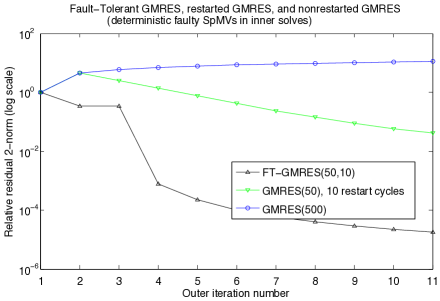
Figure 2: FT-GMRES vs. GMRES on Diagonal.

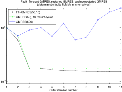
Figure 3: FT-GMRES vs. GMRES on Ill_Stokes.

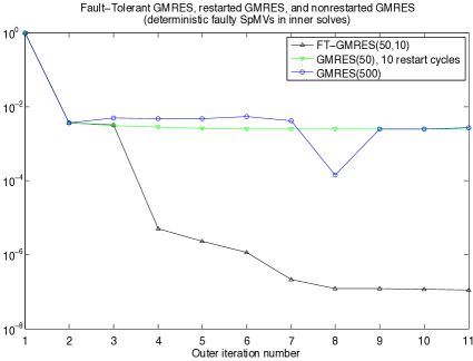
Figure 4: FT-GMRES vs. GMRES on mult_dcop_03.

Figures 2, 3, and 4 compare FT-GMRES (50 iterations per inner solve, 10 inner solves) with restarted GMRES (50 iterations per restart cycle, 10 restart cycles) and nonrestarted GMRES ($500=50\cdot 10$ iterations). Every first and third out of 10 SpMVs in GMRES, and in FT-GMRES’ inner solves, are faulty. In all cases, FT-GMRES converges faster than the other two methods, and faults cause restarted GMRES to stagnate or converge more slowly than FT-GMRES. Nonrestarted GMRES’ residual norm often fails to be monotonic. Figures 5, 6, and 7 show only FT-GMRES (50 iterations per inner solve, 20 inner solves), with different fault rates for SpMV operations in the inner solves: no faults, 1 out of 10, 3 out of 10, and 5 out of 10 SpMVs faulty. We found that increasing the fault rate only decreases the FT-GMRES convergence rate gradually. Finally, Figure 8 shows that, barring one outlier, the number of outer iterations to attain a given convergence rate increases little as the fault rate increases.

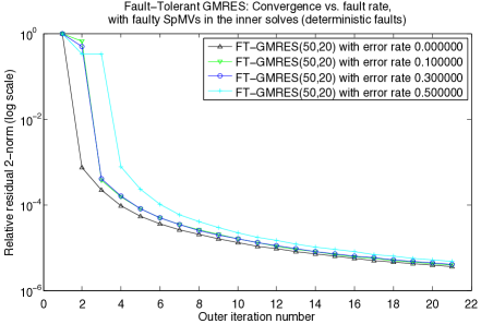
Figure 5: FT-GMRES on Diagonal problem, with different fault rates in inner solves’ SpMVs.

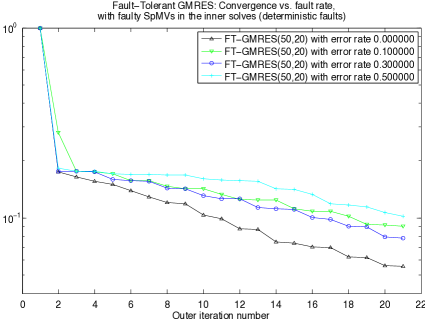
Figure 6: FT-GMRES on Ill_Stokes problem, with different fault rates in inner solves’ SpMVs.

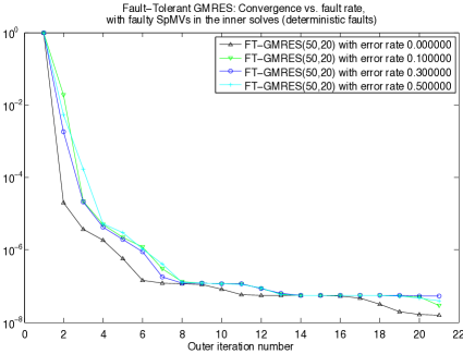
Figure 7: FT-GMRES on mult_dcop_03 problem, with different fault rates in inner solves’ SpMVs.

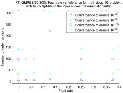
Figure 8: Number of outer iterations to convergence for FT-GMRES (50 iterations per inner solve, max 300 outer iterations) on mult_dcop_03 problem, vs. fault rate in the inner solves’ SpMVs, and the outer solves’ convergence tolerance.

9 Application / OS interface

This section describes the interface between the application and the operating system that implements a subset of the fault detection and recovery model described in Section 7. In Section 9.1, we present the interface itself. Section 9.2 outlines the implementation of this interface. Finally, we explain in Section 9.3 our technique for injecting artificial faults, which we use to test both the interface and also our FT-GMRES performance prototype. We describe fault detection separately from fault injection, in order to emphasize that our fault detection interface can work for actual memory faults as well as those which the injection framework described in Section 9.3 injects.

Our fault detection interface between the system and the application supports both actual and artificially injected memory faults. This means that the FT-GMRES implementation is ready for use with existing hardware and applications. However, the implementation of the system-application interface currently depends on artificial fault injection in order to be implemented in user space on Linux. Removing this limitation is technically possible, but requires operating system modifications, which prevents us from running tests on computers we do not administer. We leave this for future work.

9.1 Design

We have designed an application / operating system (OS) interface to support the fault and recovery models described in Section 7, and implemented a library to provide this interface. Our key design goals were to provide a simple interface for applications and algorithmic libraries, and to support existing OS-level interfaces to handling memory errors such as those provided by Linux.

/* Register callback for handling failure in a specific
 * allocation of failable memory at a specified byte offset
 * and length. arg is an opaque user-supplied argument. */
typedef void (*memfail_callback_t)( void *allocation,
                                    size_t offset,
                                    size_t len,
                                    void *arg);
void memfail_recover_init( memfail_callback_t cb, void *arg );

/* Mark resp. unmark memory as "failable" that was allocated
   with malloc().  Such memory should be freed with free(). */
void * malloc_failable( size_t len );
void free_failable( void *addr );

Figure 9: Application / Library interface to handle DRAM memory failures

This application level of this interface, shown in Figure 9, focuses on marking or unmarking contiguous memory regions that were allocated at run time using malloc(). In particular, the interface provides the application with separate calls for marking or unmarking allocations as failable memory – that is, memory in which failures will cause notifications to be sent to the application, rather than the usual fail-stop behavior of killing the application. In addition, the application also registers a callback with the library. The callback is called once for every active allocation when the library is notified by the OS of a detected but uncorrected memory fault in that allocation.

In addition to this interface, we also provide a simple producer-consumer bounded ring buffer that the application can use to queue up a sequence of failed allocations when signaled by the library. This ring buffer is non-blocking and atomic to allow asynchronous callbacks from the library to enqueue failed allocations that will be fully recovered at the end of an iteration. The application determines the size of this buffer when it is allocated; the number of entries needed must be sufficient to cover all of the allocations that could plausibly fail during a single iteration. For applications with relatively few failable allocations, this should be a minimal number of entries.

At the OS level, the library first notifies the operating system that it wishes to receive notifications of DRAM failures, either in general or in specific areas of its virtual address space depending upon the interface provided by the operating system. Second, the library keeps track of the list of failable memory allocated by the application so that it can call the application callback for each failed allocation when necessary. Finally, the library handles any error notifications from the operating system (e.g., using a Linux SIGBUS signal handler) and performs OS-specific actions to clear a memory error from a page of memory if necessary prior to notifying the application of the error.

9.2 Implementation

We added support for handling signaled memory failures as described in the previous section to an existing incremental checkpointing library for Linux, libhashckpt [16]. The library also helps track application memory usage, and provides checkpointing functionality to recover from memory failures for applications that cannot. Its ability to trap specific memory accesses eases the testing of simulated memory failures, as described later in Section 9.3. Future work may include using libhashckpt to implement efficient local save and restore of failable data. We modified libhashckpt to add the application API calls listed previously in Figure 9, with routines to mark or unmark memory as failable. This allocator also keeps a data structure sorted by allocation address of failable memory allocations.

Our fault detection system assumes that when the memory controller detects an error which ECC cannot correct, the controller notifies the operating system using a signal that indicates which cache line in which memory page failed. Linux notifies the library of DRAM memory failures, particularly failures caught by the memory scrubber using a SIGBUS signal that indicates the address of the memory page which failed. The library then unmaps this failed page using munmap(), maps in a new physical page using mmap(), and calls the application-registered callback with appropriate offset and length arguments for every failable application allocation that overlapped with the page that included the failure.

Note that Linux currently only notifies the application of DRAM failures detected by the memory scrubber. When the memory controller raises an exception caused by the application attempting to consume faulty data, Linux currently kills the faulting application. In addition, Linux only notifies applications of the page that failed and expects the application to discard the entire failed page. This approach is overly restrictive in some cases, as the hardware notifies the kernel of the memory bus line that failed, and some memory errors are soft and could be corrected simply by rewriting the failed memory line. This is not a limitation of the interface, but of the Linux operating system itself.

9.3 Fault injection

To provide support for testing DRAM memory failures, we added support to the incremental checkpointing library for simulating memory failures. In particular, we added code that randomly injects errors at a configurable rate into the application address space and uses page protection mechanisms, i.e., mprotect(), to signal the application with a SIGSEGV when it touches a page to which a simulated failure has been injected. The library then catches SIGSEGV and proceeds as if it had received a memory failure on the protected page. We model the occurrence of faults with a Poisson distribution, with a user-specified rate (faults per MB per hour). We model fault locations with a uniform distribution over all failable memory regions (i.e., those under control of our fault detection system). Faults that would occur in memory not currently marked failable are not injected.

We also implemented a software simulation of a memory “patrol scrubber” in the library. The software scrubber can asynchronously inject memory failures into the application by signaling the library when it scrubs a memory location at which a failure has been simulated. For each MPI process, we start a thread for injection. Every millisecond, that thread wakes up. (We use the POSIX Realtime Extension’s nanosleep() method to implement low-overhead sleeping.) The thread computes the number of faults that should have been injected since the last time the thread woke up, and then injects that many faults. Thus, fault occurrence “discretizes” the Poisson distribution, rather than obeying it exactly. Waking up the injection thread at longer intervals reduces its performance impact.

10 Performance prototype

In this section, we describe the implementation details of our performance prototype of FT-GMRES. We call it a performance prototype because while it may lack some features of a production-ready implementation, we expect it to have comparable performance. In particular, our solver uses the same linear algebra computational kernels and data structures as other production-ready iterative solvers. We made only minimal modifications to the linear algebra objects in order to support a fault-tolerant programming model; see the rest of this section for details. Using the same linear algebra objects means that when we turn off fault injection and detection, our implementation has the same performance characteristics as that of any other iterative solver in Trilinos. Second, our solver gains all the features of the linear algebra library “for free”: in this case, hybrid distributed- and shared-memory parallelism. Third, we can exploit libraries that use the linear algebra objects in order to use our solver in a more realistic way. For example, our performance results in Section 11 use a nontrivial incomplete factorization preconditioner, and we can inject and detect faults in the preconditioner as well. Our solver even has the same interface as other iterative solvers in Trilinos, so it may even be embedded in a real application without code changes.

We call our implementation a “prototype” because it does not attempt to handle all the kinds of hardware faults that we think the FT-GMRES algorithm could handle, given the right system support. In particular, our system library can only intercept machine check exceptions resulting from detected but uncorrectible DRAM faults. Our fault injection framework only injects faults of this kind. In Section 7.5, we argue that at least for Krylov subspace methods, bit flips are a good model for all kinds of hardware faults, including faulty arithmetic and corrupted messages. While our current run-time system may not be able to handle such faults, our more general programming model can.

10.1 Implementation outline

Our prototype relies on the application / OS interface presented in Section 9. The solver is built using components from a slightly modified version of the Trilinos solvers framework [20]. We use the implementations of GMRES [37] and Flexible GMRES [34] in Trilinos’ Belos package [7] for the inner resp. outer solvers. We preconditioned the inner iterations using the implementation of the ILUT preconditioner [35] in Trilinos’ Ifpack2 package [46]. All of these algorithms use the hybrid-parallel (threads + MPI) distributed sparse matrix and dense vector objects provided by Trilinos’ Tpetra package [4, 5]. Implementing the fault model required minor modifications to the aforementioned four Trilinos packages, in order to demonstrate a working linear solver. These modifications suffice to deploy FT-GMRES for use by any application that employs Trilinos’ Tpetra linear algebra stack, and the application would only interact with them by requesting FT-GMRES as the solver. Our entire solver prototype required only about 3000 lines of code, not including the minor Trilinos modifications.

10.2 The Failable interface

In order for FT-GMRES to control reliability of the inner and outer solves, we modified Trilinos to make all the large linear algebra objects that the solver users – the sparse matrix $A$, the preconditioner, and vectors – implement a Failable abstract interface. The Failable interface has methods for marking, unmarking, and checking whether the object’s data are allowed to experience bit flips. FT-GMRES mark failability of the relevant objects on entry to the inner solver, and unmarks them on exit. We describe below how we implemented this high-level interface using the low-level application / OS interface presented in Section 9.

Trilinos is built on the Petra framework of distributed linear algebra objects. Petra has two implementations: Epetra (Essential Petra), and Tpetra (Templated Petra). We use only Tpetra for our prototype, because Tpetra’s intranode parallel support library, Kokkos [6], has the necessary features to support our desired programming model. In particular, Kokkos allows us to intercept allocation and deallocation of large memory arrays, called compute buffers. Linear algebra objects such as sparse matrices, vectors, and preconditioners use compute buffers exclusively to store data on which they plan to execute parallel kernels. This lets us restrict where memory faults may occur, with minimal changes to the code of affected linear algebra objects. Kokkos also handles intranode parallelism in a generic way that encompasses both multicore CPU and GPU-based hardware. (In fact, this is why Kokkos needs control of memory allocation; it may need to place data on a GPU or other accelerator with a separate memory space from the CPU.) This lets our FT-GMRES prototype use hybrid parallelism (MPI and a threading library of our choice) without additional effort. Our software prototype currently works with multiple CPU-based threading libraries; we do not currently have GPU fault detection or injection capability, but this could be added at the level of the application / OS interface without changing our Trilinos modifications.

We first extended the Kokkos interface to support marking or unmarking a compute buffer as “failable.” This operation directly invokes the application / OS interface discussed in Section 9. Our Kokkos extension gives us two ways to mark failability. We may either mark or unmark all subsequent allocations of compute buffers of a particular type (e.g., double) as failable, or mark or unmark a particular compute buffer. The first option lets us experiment with faults in Tpetra-based libraries without modifying their code. (For example, we can compute the sparse matrix $A$ reliably, then intercept final assembly so that the matrix data are stored unreliably.) The second option – marking each buffer individually – lets us extend Tpetra linear algebra objects to implement the Failable interface.

We then made Tpetra sparse matrices (CrsMatrix) and dense vectors (MultiVector) implement the Failable interface. Just like compute buffers, Failable objects may be marked or unmarked failable. Certain data in the object may experience memory faults only if the object is currently marked failable. Marking a Failable object consisting of compute buffers means marking some of its compute buffers. The object’s implementation gets to control which compute buffers may experience faults. For example, our sparse matrices only mark their entries, not the sparsity structure. We can also compose more complicated Failable objects out of simpler Failable objects. For example, an ILUT incomplete factorization preconditioner consists of two sparse matrices (the $L$ and $U$ factors); marking the preconditioner failable means marking the $L$ and $U$ factors accordingly. We modified Ifpack2’s ILUT preconditioner in this way. Finally, we added an option to Belos’ GMRES solver, whether to allow memory faults in its Krylov basis vectors. This option was enabled for inner solves in all of our performance experiments in Section 11. By analogy, this makes GMRES implement Failable.

10.3 Proxy for local checkpointing

FT-GMRES needs to recover the correct the sparse matrix and preconditioner after exit of each inner solve. We implement this using a local checkpointing scheme for failable data in the sparse matrix and preconditioner, as we mentioned in Section 7. We only save the sparse matrix values, not the sparsity structure, since we only allow the values to experience memory faults. Since we do not currently have a test machine with a reliable persistent local store, our recovery method stores the “backup” in nonfailable memory as a proxy. This serves as a performance upper bound. We also used this method for saving and restoring Ifpack2’s ILUT preconditioner, since it stores its factors as Tpetra sparse matrices. This particular preconditioner is local, so we could have just recomputed it. However, many preconditioners are not local, and recomputing them often requires communication. (The coarse-grid operators in algebraic multigrid are a good example.) Moreover, recomputing the ILUT incomplete factorization each time would be expensive.

While the application / OS interface allows us to implement local approximate repair of sparse matrix values, as described in Section 7.3, we have not yet implemented this technique. The only repair we currently perform is to refresh all the sparse matrix values from reliable backing store on exit from the inner solve.

10.4 Operator wrappers

In our MATLAB-based numerical experiments (see Section 8.1), we scan the vector output of each sparse matrix or preconditioner application for invalid floating-point values (Inf or NaN), and replace them with random data. In our performance prototype, we implement a similar filter. In order to allow thread-parallel application of the filter without a thread-safe pseudorandom number generator, we implement “repairing” the vector by replacing an invalid value with the arithmetic mean of its nearest valid neighbors (within a fixed-size window of neighbors). We use the Kokkos parallel framework to apply this kernel in parallel.

11 Performance experiments

In this section, we present the results of experiments with our FT-GMRES performance prototype. We demonstrate the solver working with multiple threads and MPI processes, using production-quality software components from the Trilinos framework.

We tested FT-GMRES using the development (10.7) version of Trilinos, on a Intel Xeon X5570 (8 cores, 2.93 GHz) CPU with 12 GB of main memory. We chose for our test matrix an ill-conditioned Stokes partial differential equation discretization Szczerba/Ill_Stokes from the University of Florida Sparse Matrix Collection (UFSMC) [15]. It has 25,187 rows and columns, 193,216 stored entries, and an estimated 1-norm condition number of $4.85\times 10^{9}$. For initial experiments, we chose a uniform $[-1,1]$ pseudorandom right-hand side.

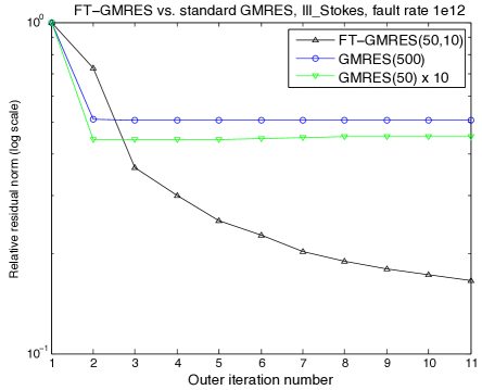
Figure 10: FT-GMRES (10 outer iterations, 50 inner iterations each), 500 iterations of non-restarted GMRES, and 10 restart cycles (50 iterations each) of restarted GMRES. (Down is good.)

We ran FT-GMRES with 10 outer iterations. Each inner solve used 50 iterations of standard GMRES (without restarting), right-preconditioned by ILUT (see e.g., Saad [36]) with level 2 fill, zero drop tolerance, 1.5 relative threshold and 0.1 absolute threshold. (These are not necessarily reasonable ILUT parameters, but they ensure a valid preconditioner for the problem tested.) We compared FT-GMRES with standard GMRES both with and without restarting: 500 iterations of each, restarting if applicable every 50 iterations. (This makes the memory usage of the two methods approximately comparable.) We set no convergence criteria except for iteration counts, so that we could fully observe the behavior of the methods. Our initial experiments use random fault injection at a rate of 1000 faults per megabyte per hour, which is high but demonstrates the solver’s fault-tolerance capabilities. Faults were allowed to occur in floating-point data belonging to the matrix and the ILUT preconditioner. Furthermore, to demonstrate the value of algorithmic approaches, our restarted GMRES implementation imitated FT-GMRES by also refreshing the matrix and ILUT preconditioner from reliable storage before every restart cycle. (We optimized by not refreshing if no memory faults were detected.)

Figure 10 shows our convergence results. FT-GMRES’ reliable outer iteration makes it able to roll forward through faults and continue convergence. The fault-detection capabilities discussed earlier in this work let FT-GMRES refresh unreliable data only when necessary, so that memory faults appear transient to the solver.

12 Conclusion

In this paper, we showed that our fault-tolerant iterative linear solver, FT-GMRES, can converge despite memory faults, whereas other iterative solvers could not. We demonstrated this both with numerical experiments using a Matlab prototype, and with a performance prototype that uses realistic fault injection and detection, implemented using production-grade solver components.

Our experiments also show that FT-GMRES’ convergence rate degrades gradually as the fault rate is increased, and that increasing the fault rate only modestly increases the total number of iterations (and therefore the total cost). While more experiments are needed, we think FT-GMRES and fault-tolerant iterative methods in general have great potential to improve solver robustness and relax hardware reliability constraints. The basic approaches we have used can be applied to many algorithms, greatly reducing the impact of the soft faults that are expected on future computing systems.

Our work has also opened up interesting collaborations with systems researchers, to develop programming interfaces for varying reliability, reporting faults, and selective checkpointing. These collaborations have the potential to influence hardware-software codesign, especially at extreme scales, where energy requirements will force system designers to reduce hardware reliability and rely more on software approaches. Fault-tolerant algorithms thus have the potential to influence computer hardware in a way analogous to RISC (Reduced Instruction Set Computer) architectures [32], by encouraging beneficial trade-offs between hardware and software.

References

- [1] K. Asanovic, R. Bodik, B. C. Catanzaro, J. J. Gebis, P. Husbands, K. Keutzer, D. A. Patterson, W. L. Plishker, J. Shalf, S. W. Williams, and K. A. Yelick, The Landscape of Parallel Computing Research: A View from Berkeley, Tech. Rep. UCB/EECS-2006-183, EECS Department, University of California, Berkeley, Dec 2006. See also the journal article Asanovic et al. [2].
- [2] K. Asanovic, R. Bodik, J. W. Demmel, T. Keaveny, K. Keutzer, J. Kubiatowicz, N. Morgan, D. A. Patterson, K. Sen, J. Wawrzynek, D. Wessel, and K. A. Yelick, A View of the Parallel Computing Landscape, Communications of the ACM, 52 (2009), pp. 56–67.
- [3] J. Bahi, S. Contasset-Vivier, and R. Couturier, Parallel Iterative Algorithms: From Sequential to Grid Computing, Chapman and Hall / CRC, 2007.
- [4] C. G. Baker, Engineering a kernel-agnostic distributed linear algebra library for multi/many-core in Trilinos. Refereed abstract in minisymposium “Parallel Programming Models and Algorithms for Scalable Manycore Systems,” SIAM Conference on Computational Science and Engineering 2011, Reno, NV, March 2011.
- [5] , Gradually transitioning library users to the hybrid-parallel paradigm. Refereed abstract in minisymposium “Creating the Next Generation of High Performance Numerical Computing Capabilities,” International Congress on Industrial and Applied Mathematics (ICIAM) 2011, Vancouver, B.C., July 2011.
- [6] C. G. Baker, H. C. Edwards, M. A. Heroux, and A. B. Williams, A light-weight API for portable multicore programming, in The 18th Euromicro International Conference on Parallel, Distributed and Network-Based Computing (PDP 2010), February 2010.
- [7] E. Bavier, M. Hoemmen, S. Rajamanickam, and H. Thornquist, Amesos2 and Belos: Direct and iterative solvers for large sparse linear systems, 2011. Submitted to Scientific Programming.
- [8] L. S. Blackford, A. Cleary, J. Demmel, I. Dhillon, J. Dongarra, S. Hammarling, A. Petitet, H. Ren, K. Stanley, and R. C. Whaley, Practical experience in the dangers of heterogeneous computing, Tech. Rep. UT-CS-96-330, University of Tennessee, Knoxville, July 1996. LAPACK Working Note #112.
- [9] , Practical experience in the numerical dangers of heterogeneous computing, ACM Trans. Math. Softw., 23 (1997), pp. 133–147.
- [10] G. Bronevetsky and B. de Supinski, Soft error vulnerability of iterative linear algebra methods, in Proceedings of the 22nd Annual International Conference on Supercomputing, ICS ’08, New York, NY, USA, 2008, ACM, pp. 155–164.
- [11] A. Buttari, J. Dongarra, J. Kurzak, P. Luszczek, and S. Tomov, Computations to enhance the performance while achieving the 64-bit accuracy, Tech. Rep. UT-CS-06-584, University of Tennessee Knoxville, November 2006. LAPACK Working Note #180.
- [12] M. Castro and B. Liskov, Practical Byzantine fault tolerance and proactive recovery, ACM Transactions on Computer Systems, 20 (2002), pp. 398–461.
- [13] G. Chen, M. Kandemir, M. J. Irwin, and G. Memik, Compiler-directed selective data protection against soft errors, in In Proceedings of the Asia and South Pacific Design Automation Conference (ASPDAC), Shanghai, China, January 2005.
- [14] Z. Chishti, A. R. Alameldeen, C. Wilkerson, W. Wu, and S.-L. Lu, Improving cache lifetime reliability at ultra-low voltages, in Proceedings of the 42nd Annual IEEE/ACM International Symposium on Microarchitecture, MICRO 42, New York, NY, USA, 2009, ACM, pp. 89–99.
- [15] T. A. Davis and Y. Hu, The University of Florida Sparse Matrix Collection, ACM Trans. Math. Softw. (to appear), (2011).
- [16] K. B. Ferreira, R. Riesen, R. Brightwell, P. G. Bridges, and D. Arnold, Libhashckpt: Hash-based incremental checkpointing using GPUs, in Proceedings of the 18th EuroMPI Conference, Santorini, Greece, September 2011.
- [17] G. H. Golub and Q. Ye, Inexact preconditioned conjugate gradient method with inner-outer iteration, SIAM J. Sci. Comput., 21 (1999), pp. 1305–1320.
- [18] A. Greenbaum, V. Ptak, and Z. Strakos, Any nonincreasing convergence curve is possible for GMRES, SIAM J. Matrix Anal. Appl., 17 (1996), pp. 465–469.
- [19] I. S. Haque and V. S. Pande, Hard data on soft errors: A large-scale assessment of real-world error rates in GPGPU, in Proceedings of the 2010 10th IEEE/ACM International Conference on Cluster, Cloud and Grid Computing, CCGRID ’10, Washington, DC, USA, 2010, IEEE Computer Society, pp. 691–696.
- [20] M. A. Heroux, R. A. Bartlett, V. E. Howle, R. J. Hoekstra, J. J. Hu, T. G. Kolda, R. B. Lehoucq, K. R. Long, R. P. Pawlowski, E. T. Phipps, A. G. Salinger, H. K. Thornquist, R. S. Tuminaro, J. M. Willenbring, A. Williams, and K. S. Stanley, An overview of the Trilinos project, ACM Trans. Math. Softw., 31 (2005), pp. 397–423.
- [21] M. A. Heroux and M. Hoemmen, Fault-tolerant iterative methods via selective reliability, Tech. Rep. SAND2011-3915 C, Sandia National Laboratories, 2011. Available at http://www.sandia.gov/~maherou/.
- [22] V. E. Howle, Soft errors in linear solvers as integrated components of a simulation, in Presented at the Copper Mountain Conference on Iterative Methods, Copper Mountain, CO, April 9, 2010.
- [23] K.-H. Huang and J. A. Abraham, Algorithm-based fault tolerance for matrix operations, IEEE Transactions on Computers, C-33 (1984).
- [24] T. Karnik, P. Hazucha, and J. Patel, Characterization of soft errors caused by single event upsets in CMOS processes, IEEE Trans. Dependable Secur. Comput., 1 (2004), pp. 128–143.
- [25] P. M. e. Kogge, ExaScale Computing Study: Technology Challenges in Achieving Exascale Systems, tech. rep., University of Notre Dame CSE Department Technical Report, TR-2008-13, September 28, 2008.
- [26] L. Lamport, R. Shostak, and M. Pease, The Byzantine Generals Problem, ACM Transactions on Programming Languages and Systems, 4 (1982), pp. 382–401.
- [27] J. Langou, Z. Chen, G. Bosilca, and J. Dongarra, Recovery patterns for iterative methods in a parallel unstable environment, SIAM J. Sci. Comput., 30 (2007), pp. 102–116.
- [28] P. T. Lin and J. N. Shadid, Towards large-scale multi-socket, multicore parallel simulations: Performance of an MPI-only semiconductor device simulator, J. Comput. Phys., 229 (2010), pp. 6804–6818.
- [29] K. Malkowski, P. Raghavan, and M. Kandemir, Analyzing the soft error resilience of linear solvers on multicore processors, in Proceedings of the Twenty-Fourth IEEE International Parallel and Distributed Processing Symposium (IPDPS), 2010.
- [30] N. Miskov-Zivanov and D. Marculescu, Soft error rate analysis for sequential circuits, in Proceedings of the Conference on Design, Automation and Test in Europe, DATE ’07, San Jose, CA, USA, 2007, EDA Consortium, pp. 1436–1441.
- [31] B. Parhami, Defect, fault, error, …, or failure?, IEEE Transactions on Reliability, 46 (1997).
- [32] D. A. Patterson and C. H. Sequin, RISC I: A Reduced Instruction Set VLSI Computer, in Proceedings of the Eighth Annual Symposium on Computer Architecture (ISCA), IEEE Computer Society Press, 1981.
- [33] M. Rosenblum, The reincarnation of virtual machines, Queue, 2 (2004).
- [34] Y. Saad, A flexible inner-outer preconditioned GMRES algorithm, SIAM J. Sci. Comput., 14 (1993), pp. 461–469.
- [35] , ILUT: a dual threshold incomplete ILU factorization, Num. Lin. Alg. Appl., 1 (1994), pp. 387–402.
- [36] , Iterative Methods for Sparse Linear Systems, SIAM, Philadelphia, second ed., 2003.
- [37] Y. Saad and M. H. Schultz, GMRES: A generalized minimal residual algorithm for solving nonsymmetric linear systems, SIAM J. Sci. Statist. Comput., 7 (1986), pp. 856–869.
- [38] B. Schroeder, E. Pinheiro, and W.-D. Weber, DRAM errors in the wild: A large-scale field study, in SIGMETRICS / Performance 2009, June 15–19, 2009, Seattle, WA, USA, 2009.
- [39] V. Simonici and D. B. Szyld, Flexible inner-outer Krylov subspace methods, SIAM J. Numer. Anal., 40 (2003), pp. 2219–2239.
- [40] , Theory of inexact Krylov subspace methods and applications to scientific computing, SIAM J. Sci. Comput., 25 (2003), pp. 454–477.
- [41] J. E. Smith and R. Nair, The architecture of virtual machines, Computer, 38 (2005), pp. 32–38.
- [42] G. W. Stewart, Updating a rank-revealing decomposition, SIAM J. Matrix Anal. Appl., 14 (1993), pp. 494–499.
- [43] D. B. Szyld and J. A. Vogel, FQMR: A flexible quasi-minimal residual method with inexact preconditioning, SIAM J. Sci. Comput., 23 (2001), pp. 363–380.
- [44] J. van den Eshof and G. L. G. Sleijpen, Inexact Krylov subspace methods for linear systems, SIAM J. Matrix Anal. Appl., 26 (2004), pp. 125–153.
- [45] J. H. Wilkinson, Rounding Errors in Algebraic Processes, Prentice Hall, Englewood Cliffs, NJ, 1963. This work has been republished in an inexpensive Dover paperback edition.
- [46] A. Williams, New Trilinos package: Ifpack2, 2010. Presentation at Trilinos Users’ Group meeting, Sandia National Laboratories, Albuquerque, New Mexico, 04 November 2010. Video available at http://trilinos.sandia.gov/events/trilinos_user_group_2010/.
- [47] S. Yang, W. Wolf, W. Wang, N. Vijaykrishnan, and Y. Xie, Low-leakage robust SRAM cell design for sub-100nm technologies, in Proceedings of the 2005 Asia and South Pacific Design Automation Conference, ASP-DAC ’05, New York, NY, USA, 2005, ACM, pp. 539–544.