Anomalous coarsening in disordered exclusion processes

Abstract

We study coarsening phenomena in three different simple exclusion processes with quenched disordered jump rates. In the case of the totally asymmetric process, an earlier phenomenological description is improved, yielding for the time dependence of the length scale $\xi(t)\sim t/(\ln t)^{2}$, which is found to be in agreement with results of Monte Carlo simulations. For the partially asymmetric process, the logarithmically slow coarsening predicted by a phenomenological theory is confirmed by Monte Carlo simulations and numerical mean-field calculations. Finally, coarsening in a bidirectional, two-lane model with random lane-change rates is studied. Here, Monte Carlo simulations indicate an unusual dependence of the dynamical exponent on the density of particles.

1 Introduction

Single-file transport is known to be susceptible to heterogeneities of the track on which the process takes place—one may think of formation of jams in vehicular traffic [1] or shocks in the intracellular traffic of molecular motors on the filamentary network [2]. Such systems are frequently modeled by some variant of the asymmetric simple exclusion process (ASEP) [3, 4], where particles jump stochastically on a lattice and interact through excluding multiple occupations on lattice sites. For this model, in its homogeneous form, many exact results are available [5, 6] and, therefore, it has become a paradigmatic model of non-equilibrium systems. Motivated by understanding transport in heterogeneous systems, the ASEP with quenched random jump rates has been the subject of ongoing research [7, 8, 9, 10, 11, 12, 13, 14, 15, 16, 17, 18]. Besides the experimental relevance, the effect of disorder on this model is also a challenging problem as general exact solutions are still lacking here, and the bulk of the results have been obtained by mean-field approximations, phenomenological theories based on extreme-value statistics and Monte Carlo simulations.

Since the ASEP can be mapped to a growth process of a $1+1$ dimensional surface [19] which is described by the Kardar-Parisi-Zhang equation [20], results for exclusion processes are also important to understand the fundamentals of surface physics [21] or directed polymers in random media [20]. Due to the steady current, the correlation length diverges in these systems and, consequently, they exhibit a non-equilibrium critical scaling behavior that can be classified into universality classes [22]. Understanding the effects of disorder on lattice gas models thus reveals the behavior of the corresponding interfaces. In particular, variants of the ASEP with quenched randomness in the hopping rates are related to surface growth models with columnar disorder (see [22]).

Typically, these models relax toward the steady state much slower than the corresponding homogeneous ones; in certain cases, the coarsening dynamics are logarithmically slow. Owing to this, confirming the predictions of phenomenological theories by Monte Carlo simulations is a very hard numerical task. As it has been recently shown, inhomogeneous exclusion processes can be parallelized and simulated efficiently on a GPU [23], similar to other interacting systems [24, 25, 26]. In this work, we shall get use of this new technique (among other methods, such mean-field approximation) in studying the dynamics of three variants of the disordered ASEP: (i) the disordered totally asymmetric simple exclusion process (DTASEP), where particles move unidirectionally, (ii) the disordered partially asymmetric simple exclusion process (DPASEP), where particles can move in both directions and (iii) a recently introduced bidirectional two-lane model, where the disorder appears in the lane-changes [27]. We shall see that the above disordered processes with parallel (or synchronous) update procedure have essentially the same physical properties as those with (the most frequently studied) random sequential (or asynchronous) update procedure. In comparing the results with the mean-field description we shall enlighten the limitations of the latter in case slow modes related to moving domain walls are present.

The paper is organized as follows. In section 2 and 3, the coarsening phenomenon in the DTASEP and in the DPASEP is investigated, respectively. Section 4 is devoted to the steady state and the coarsening in the bidirectional two-lane model. Finally, results are discussed in section 5. Some technical details concerning the parallelization are given in the Appendix.

2 Coarsening in the disordered totally asymmetric simple exclusion process

First, we shall study the disordered totally asymmetric simple exclusion process defined as follows. A one-dimensional periodic lattice with $L$ sites is given, on which $N$ particles reside, at most one on each site. The TASEP is a continuous-time stochastic process in which particles move from site $i$ to site $i+1$ independently with rate $p_{i}$ provided site $i+1$ is empty. The jump rates $p_{i}$ are independent random variables drawn from a bimodal distribution:

$$f(p_{i})=(1-\phi)\delta(p_{i}-1)+\phi\delta(p_{i}-r)\ \ ,$$ (1)

where $0<r<1$ and $0<\phi<1$. Although exact solutions are lacking for this model, the main features of the steady state and the non-stationary (coarsening) behavior are well understood by means of a phenomenological description [12, 16]. This rests on that particles accumulate behind consecutive stretches of bonds with rate $p_{i}=r$ (called bottlenecks) and form a high density domain where the local density is greater than $1/2$. Provided that the global density $N/L$ is close to $1/2$, and the system is initiated in a state with a uniform density, then high-density segments form behind bottlenecks and start to grow as time elapses. During this process, segments at short bottlenecks lose particles in favor of those at longer ones until the former gradually vanish. Ultimately, provided the system was finite, a single, macroscopic high density domain accumulates behind the longest bottleneck while in the rest of the system the local density is below $1/2$. So, the system undergoes a coarsening process which is characterized by the dependence of the typical size of segments $\xi(t)$ on time. In a simplified description of this phenomenon, the bottlenecks are treated to be independent and are characterized by a (length dependent) maximal current. Furthermore, the essence of the coarsening process is captured if one concentrates merely on the evolution of length of high density segments behind bottlenecks. Under these assumptions, the model reduces to a disordered zero-range process [28], where the dynamical exponent $z$ describing the coarsening as

$$\xi(t)\sim t^{1/z}$$ (2)

is known to depend on the asymptotics $\rho(w)\sim(w-c)^{n}$ of the distribution of jump rates at the lower edge $c$ as $z=(n+2)/(n+1)$ [29]. In the DTASEP, the maximal current through a bottleneck of length $l$ is [30]

$$J(l)=r/4+O(l^{-1})$$ (3)

and the distribution of the bottleneck length is geometric. This yields formally $n=\infty$ and $z=1$. In this special limit, non-rigorous arguments based on extreme value statistics indicate that the coarsening is not simply linear but logarithmic corrections arise as $\xi(t)\sim t/\ln t$ [12].

Here, we shall reconsider this reasoning and refine it by applying the statistics of extremes in a more precise way. Let us consider a growing high-density segment of length $\xi_{i}(t)$. Clearly, the rate of growth of $\xi_{i}(t)$ is determined the difference $\Delta J_{i}$ between the current $J_{i-1}$ through the bottleneck on the left hand side of the growing segment and the current $J_{i}$ through the bottleneck on its right hand side:

$$\dot{\xi_{i}}(t)\sim\Delta J_{i}.$$ (4)

The two bottlenecks are separated by a distance $O(\xi(t))$ and, in this domain, the bottleneck on the right hand side is the longest one (having length $l_{1}$) and the other one is the second longest one (having length $l_{2}$). Using Eq. (3), the current difference can be written in terms of bottleneck lengths as

$$\Delta J_{i}\sim 1/l_{2}-1/l_{1}=(l_{1}-l_{2})/l_{1}l_{2}.$$ (5)

Approximating, for the sake of simplicity, the geometric distribution of bottleneck lengths by the continuous exponential distribution $P_{<}(l)=1-e^{-\ln(1/Q)l}$, it is straightforward to show that the most probable values of $l_{1}$ and $l_{2}$ among $\xi$ events, $l_{1}^{*}\approx\ln\xi/\ln(1/Q)$ and $l_{2}^{*}\approx\ln(\xi/2)/\ln(1/Q)$, respectively, are shifted by a finite value. Furthermore, the variances of the distributions of $l_{1}$ and $l_{2}$ tend to finite values in the limit $\xi\to\infty$. Therefore the limit distribution of $l_{1}-l_{2}$ also has a finite most probable value and variance and, consequently, the typical current difference scales with $\xi$ as

$$\Delta J_{i}\sim 1/l_{1}l_{2}\sim 1/(\ln\xi)^{2}$$ (6)

for large $\xi$. Putting this into Eq. (4) and integrating yields for the growth of $\xi(t)$

$$\xi(t)\sim t/(\ln t)^{2}$$ (7)

in leading order for long times.

For measuring the typical length of segments we have made use of a well-known relationship between the ASEP and a simple one-dimensional surface growth model where height differences $\Delta h_{i}=h_{i+1}-h_{i}$ are related to the occupation number $n_{i}$ of the ASEP as $\Delta h_{i}=2n_{i}-2N/L$ [19]. A usual measure of the width of the surface is given by

$$W(L,t)=\Bigl{[}\frac{1}{L}\,\sum_{i=1}^{L}\,h^{2}_{i}(t)-\Bigl{(}\frac{1}{L}\,\sum_{i=1}^{L}\,h_{i}(t)\Bigr{)}^{2}\Bigr{]}^{1/2}\ .$$ (8)

In case of the coarsening DTASEP, the equivalent surface consists of roughly linearly ascending and descending parts corresponding to high and low density segments, respectively. Therefore the quantity given in Eq. (8) is proportional to the typical value of $\xi(t)$.

We performed numerical simulations of the model both with random sequential updates and parallel sub-lattice updates (see the Appendix) and used the bimodal distribution with parameters $\phi=1/2$ and $r=1/4$. The density of particles was $N/L=1/2$. We have considered systems with size $L=16000$ and $L=48000$ and measured the time evolution of the surface width. The average of $W(L,t)$ is plotted against $t/(\ln t)^{2}$ in Fig. 1.

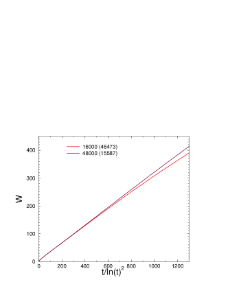
Figure 1: Dependence of the surface width of the DTASEP on time, obtained by Monte Carlo simulations with parallel updates for $L=16000,48000$. The number of independent samples are given in parentheses.

Here, a linear dependence can be seen for not too long times, where finite size effects are negligible. Data for finite sizes satisfactorily follow the scaling law

$$W(L,t)=L\tilde{W}(t/(\ln t)^{2}/L),$$ (9)

see Fig. 2, although, with strong corrections to scaling.

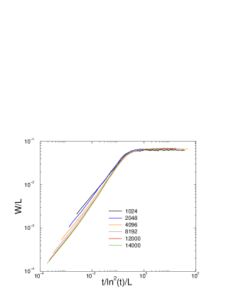
Figure 2: Scaling plot of the width $W(L,t)$ obtained for different system sizes by Monte Carlo simulations with parallel updates.

In order to compare the prediction in Eq. (7) with numerical results more precisely we have calculated the effective dynamical exponent by $1/z_{\rm eff}(t)=d\ln W(t,L)/d\ln t$. Due to the logarithmic factor in Eq. (7), the leading order correction term in the finite-time effective exponent is slowly decaying, having the form

$$1/z_{\rm eff}(t)=1-2/\ln t+\cdots$$ (10)

in an infinite system.

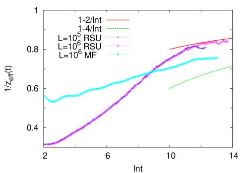
Figure 3: Effective dynamical exponents plotted against time obtained by Monte Carlo simulations with random sequential updates (+,$\times$) and by numerically solving the numerical mean field equations ($\ast$). The curves correspond to the predictions of the phenomenological theory.

As can be seen in Fig. 3, for moderate time scales the effective exponents still deviate from the predictions of the simple phenomenological theory, nevertheless, the agreement with Eq. (10) is satisfactory for long times. Due to the slow, logarithmic convergence, the estimates on the exponents obtained on small scales differ significantly from the asymptotic values, see the numerical results in Ref. [31].

Note, that the simplest scaling hypothesis for roughening surfaces, which is valid for, among others, the above model in the absence of disorder is of the form

$$W(L,t)=L^{\alpha}\tilde{W}(t/L^{z})$$ (11)

rather than that given Eq. (9). Here, according to the usual terminology, $\alpha$ is the roughness exponent characterizing the finite-size scaling of the stationary width of the surface, i.e. $W(L,t\to\infty)\sim L^{\alpha}$, while the surface growth exponent $\beta=z/\alpha$ describes the evolution of the surface width in an infinite system for long times as $W(L\to\infty,t)\sim t^{\beta}$. Hence, apart from the logarithmic correction, the surface growth model corresponding to the DTASEP is characterized by the exponents $\alpha=\beta=z=1$.

We have also studied the model within a mean-field approximation in which the expected values $\langle n_{i}(t)n_{i+1}(t)\rangle$ in the master equation of the process are replaced by $\langle n_{i}(t)\rangle\langle n_{i+1}(t)\rangle$. Then the master equation turns into the following evolution equations for the local densities $\rho_{i}(t)\equiv\langle n_{i}(t)\rangle$

$$\frac{d\rho_{i}}{dt}=p_{i-1}\rho_{i-1}(1-\rho_{i})-p_{i}\rho_{i}(1-\rho_{i+1}),\qquad i=1,2,\dots,L.$$ (12)

This approximation gives the general features of the ASEP correctly, but, since the correlations are neglected, it may yield incorrect critical exponents. From the point of view of the above phenomenological theory an important difference is that the finite-size corrections of the current in the mean-field model are in the order of $l^{-2}$ [31], rather than $l^{-1}$, see Eq. (3). Repeating the above calculations otherwise unchanged, leads to a different outcome for the form of the logarithmic correction; one obtains namely $\xi(t)\sim t/(\ln t)^{4}$ and, correspondingly, $1/z_{\rm eff}(t)=1-4/\ln t+\cdots$. We have solved Eqs. (12) numerically by using the 4th order Runge-Kutta method for $10^{2}$ samples with $L=10^{6}$. The calculated effective exponents are compared with the predictions of the theory in Fig. 3. As can be seen, on the time-scales of the numerical investigation a deviation from the predictions is present, which is, however, decreasing with increasing time.

3 Coarsening in the disordered partially asymmetric exclusion process

The dynamics are much different in the quenched disordered partially asymmetric exclusion process (DPASEP), where particles can move in both directions with random rates $p_{i}$ and $q_{i}$ to the right and to the left, respectively, from site $i$ [9, 8, 14, 16]. Here, due to the large fluctuations of the random potential landscape [32], which is itself a random walk, the displacement of a single particle increases ultra-slowly as

$$\overline{\langle x^{2}(t)\rangle}\sim(\ln t)^{2/\psi},$$ (13)

with the barrier exponent $\psi=1/2$, when the average force $F=\overline{\ln{(p_{i}/q_{i+1}})}$ acting on the particle is zero [33]. Here, $\langle\cdot\rangle$ denotes an average over different stochastic histories, whereas the overbar denotes an average over the random transition rates. In the following, we shall restrict ourselves to the unbiased case, i.e. $F=0$. In the presence of many particles (i.e. in the DPASEP), numerical simulations showed that the motion of a tagged particle follows the same law given in Eq. (13) [8] and, in accordance with the activated dynamics, the stationary current in finite rings of size $L$ behaves as [14]

$$-\ln|J(L)|\sim L^{\psi}.$$ (14)

When the system starts from a homogeneous state it shows a coarsening phenomenon similar to the DTASEP. Queues form at potential barriers, where the local density is close to one, leaving the rest of the lattice almost completely empty. As time elapses, queues at smaller barriers gradually dissolve and particles accumulate behind larger and larger barriers. Scaling considerations based on the finite-size scaling behavior of the current in Eq. (14) lead to that the typical size of high-density segments increases with time in an infinite system as [14]

$$\xi(t)\sim\ln^{1/\psi}[t/\ln(t)].$$ (15)

This means that the corresponding surface is characterized formally by the exponents $\alpha=1$, $\beta=0$ and $z=\infty$. We mention that, in the presence of a bias ($F>0$), the scaling is normal, i.e. has the form given in Eq. 11, with $\alpha=1$ and with $\beta$ and $z$ continuously varying with $F$ [14].

Our aim here is to test the coarsening law in Eq. (15) by measuring the dependence of the corresponding surface width $W(t)$ in Monte Carlo simulations. Numerical results obtained with the parallel updating procedure for different system sizes are shown in Fig. 4. As can be seen, not considering long times where the data are affected by the finite size of the system, the results are compatible with the law given in Eq. (15).

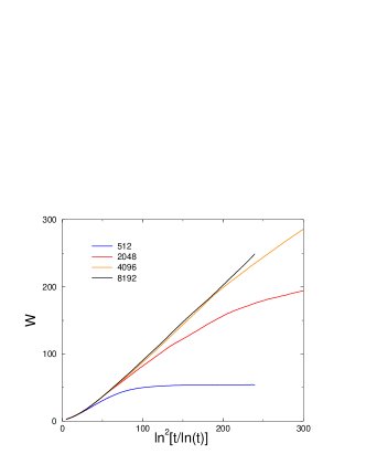
Figure 4: Dependence of the surface width of the DPASEP on time, obtained by Monte Carlo simulations for sizes $L=512,2048,4096,8192$.

We have also considered the model within the mean-field approximation, which has recently been demonstrated to describe both the stationary behavior and the dynamics of the model correctly [18]. The dynamical mean-field equations read for this model as

$$\frac{d\rho_{i}}{dt}=(p_{i-1}\rho_{i-1}+q_{i}\rho_{i+1})(1-\rho_{i})-[p_{i}(1-\rho_{i+1})+q_{i-1}(1-\rho_{i-1})]\rho_{i}.$$ (16)

In the earlier work, the coarsening length scale has been studied within the mean-field approximation indirectly by measuring the typical distance between adjacent peaks in the density profile [18]. Here, we have solved the equations Eqs. (16) numerically and calculated directly the surface width $W(t)$ as a function of time. Results shown in Fig. 5 are in good agreement with Eq. (15).

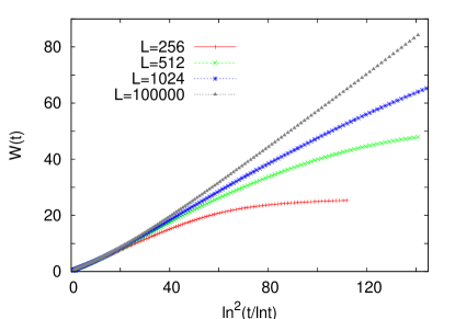
Figure 5: The same plot as in Fig. 4, but the data are obtained by solving the dynamical mean-field equations. The number of samples was $10^{2}$.

4 Dynamics of a bidirectional, two-lane exclusion process with random lane-change rates

4.1 Definition of the model and preliminaries

In the final part of this work, we shall study a recently introduced bidirectional, two-lane exclusion process, where the lane-change rates are random variables [34, 27]. The precise definition of the model is given as follows. Two parallel, one-dimensional, periodic lattices are given, each of them with $L$ sites. Particles move within a lane unidirectionally, following the dynamical rules of the TASEP with unit jump rates but the directions of motion in the two lanes are opposite. In addition two this, particles change lanes from site $i$ of lane A(B) to the neighboring site of lane B(A) with rate $u_{i}$($v_{i}$) provided the target site is empty. The model and its possible transitions are illustrated in Fig. 6.

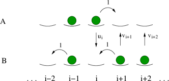
Figure 6: Sketch of the bidirectional, two-lane model under study. Allowed transitions with the corresponding rates are indicated.

Notice that the direction of motion of particles can be regulated in this model by tuning the asymmetry in the lane-change rates. This arrangement was intended to model traffic of molecular motors moving along oppositely oriented filaments, which can be realized in experiments and may be relevant with respect to in vivo processes [35]. A single motor in this environment with homogeneous and symmetric lane-change rates performs normal diffusion, however, with an enhanced diffusion coefficient compared to that of the symmetric random walk [36]. Recently, the model has been reinterpreted as a model of motors able to move bidirectionally along the filament [37].

We shall consider the disordered version of the above model where the pairs of rates $(u_{i},v_{i})$ are i.i.d. random variables. In case there is only a single particle in the system, one can introduce an effective potential, say, in lane A,

$$\Delta U_{i}\equiv U^{A}_{i}-U^{A}_{i-1}=\ln\frac{1+u_{i}}{1+v_{i}},$$ (17)

hence, the problem is essentially reduces to a one-dimensional random walk in the presence of the above potential field [27]. If $\overline{\Delta U_{i}}=0$, the time dependence of the displacement follows Sinai’s law given in Eq. (13) with $\psi=1/2$. What makes the model with many particles difficult is that no effective potential exists in that case and we have a genuine non-equilibrium process. An interesting consequence is the following. Having one particle in a finite, periodic system where the effective potential is single-valued, i.e. $U_{1}=U_{L+1}$, the expected velocity of the particle will be zero. But when putting more particles in the same system, the reduction to an effective potential field does not work anymore, and the expected velocity (or current) of particles will be non-zero (except when the sequence of random rates has a left-right symmetry). This interaction induced bias makes difficult to find a general criterion for the unbiased point $\overline{J}=0$ in terms of the distribution of lane-change rates. Nevertheless, a sufficient condition for this is that the joint distribution of rates $P(u,v)$ is symmetric under the interchange of $u$ and $v$. In the following we will focus on this case, which has not been studied so far.

The model has exclusively been investigated in the driven phase, where $\overline{J}\neq 0$ in finite periodic systems. It has been found that the steady state at a bottleneck with $u>v$ (while in the rest of the system $v>u$), is much different from that of the one-lane partially asymmetric exclusion process PASEP. In the latter, the front of the high-density cluster is localized, leading to an exponentially decreasing current with the size $l$ of the bottleneck, whereas in the former the front performs a symmetric random walk, resulting in a larger current in the order of $l^{-1}$ [27]. Based on this, the current in the driven phase of the disordered model was predicted to decay with the system size $L$ as $J(L)\sim 1/\ln L$, rather than the much faster algebraic decay in the corresponding phase of the one-lane DPASEP. Therefore, owing to the collective diffusive motion of the high-density cluster, particles overcome barriers more efficiently in the two-lane model than in the one-lane PASEP. We aim here at investigating whether this effect is present at the unbiased point. Since the phenomenological theory based on independent barriers breaks down here, we will resort to numerical methods.

4.2 Steady state

A special property of this model, which is due to a symmetry, is that if $N=L$, the stationary current is exactly zero for any set of the lane-change rates, and the local densities fulfill $\langle n_{i}^{A}\rangle=1-\langle n_{i}^{B}\rangle$ [27]. If the global density is smaller than $1/2$, the stationary current is non-zero (but vanishing in the limit $L\to\infty$) and the steady state is segregated, consisting of a half-filled domain where approximately $\langle n_{i}^{A}\rangle+\langle n_{i}^{B}\rangle\approx 1$ and a zero-density domain, where the density is almost zero. An appropriate measure of typical size of the half-filled domain is the corresponding surface width, but now the surface increment is related to the occupation numbers as $\Delta h_{i}=2(n_{i}^{A}+n_{i}^{B})-2N/L$. As it is clear from the above picture, the surface width in the steady state is proportional to the system size, i.e. $W(L,t\to\infty)\sim L$ for $N\neq L$. The steady state is, however, much different at half-filling ($N=L$). In that case, the half-filled phase covers the entire system, thus the mean profile $\langle n_{i}^{A}\rangle+\langle n_{i}^{B}\rangle$ is flat, like in a homogeneous system where $u_{i}=v_{i}=1$. As a comparison, we have investigated the homogeneous system by Monte Carlo simulations (data not shown) and found the surface width to obey the scaling relation $W(L,t)=L^{1/2}\tilde{W}(t/L^{2})$ for any density, similar to the symmetric simple exclusion process belonging to the Edwards-Wilkinson universality class [38]. Thereby one would expect the surface width in the disordered model for $N=L$ to be reduced, compared to that at other densities. Surprisingly, numerical simulations still indicate $W(L,t\to\infty)\sim L$, which refers to large fluctuations. The reason for this is the following. Besides the half-filled state, there are two other states, in which the current is trivially zero: the empty and the full lattice. In a half-filled system ($N=L$), let us imagine a state consisting of half-filled segments with $\langle n_{i}^{A}\rangle=1-\langle n_{i}^{B}\rangle$, as well as empty and fully occupied segments. In the homogeneous model, this state will not be stable (i.e. a steady state) since particles penetrate into the empty segments, just as holes into fully occupied segments and move there with a finite velocity for $u\neq v$, leading to that these segments ultimately dissolve and the whole system is occupied by the half-filled phase. In a disordered system, however, the half-filled phase is unstable. Here, fully occupied and empty segments are able to form spontaneously due to inhomogeneities and live for long times.

To illustrate this phenomenon, let us consider a caricature of a disordered system, which contains just two extended regions (called reverse bias regions) of length $l$, where $u>v$, and which are far from each other, while in the rest of the system $v>u$, see Fig 7.

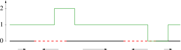
Figure 7: Snapshot of the density profile $\langle n_{i}^{A}\rangle+\langle n_{i}^{B}\rangle$ (green line) in a system consisting of two reverse bias regions (denoted by the dashed red sections). The arrows indicate the direction of motion of particles in the empty lattice and holes in the occupied lattice.

An interesting property of the model under study is that a particle in an otherwise empty region and a hole in an otherwise occupied region move in the same direction; from left to right (from right to left) if $v>u$ ($u>v$). Let us assume, that a small empty segment appears around the right end point of one of the reverse bias regions. This segment (or condensate of holes) is stable, as particles, penetrating into this segment from the surrounding half-filled phase (either from left or from right) move preferably away from the end point, i.e. they are forced back into the half-filled phase. So the domain walls, separating the empty segment from the surroundings are stable. Of course, due to the conservation of particles, a fully occupied segment must emerge at the right end point of the other reverse bias region, which will be stable, as well, from similar reasons given above. Although the mean particle current through the half-filled phase in between the two reverse bias regions is zero, its fluctuations result in that the size of empty and fully occupied segments fluctuates (in a correlated way due to particle conservation), as well. The empty (or the fully occupied) region can extend over a length of $l$ on both sides of the right end point of the reverse bias region, independently. These correlated fluctuations of the size of particle (and hole) condensates at the two reverse bias regions amount to a net displacement of particles from one reverse bias region to the other one and lead to fluctuations of the corresponding surface.

Concerning the inhomogeneous model, it can be divided into effective forward and reverse bias regions, where for the majority of links $v_{i}>u_{i}$ and $v_{i}<u_{i}$ hold, respectively. Therefore, similar fluctuations occur as in the above simplified system. The largest effective reverse bias region is macroscopic in the unbiased case [27], hence the surface width must scale linearly with the system size, in accordance with the observations.

4.3 Coarsening

When the system is started from a homogeneous initial state, a coarsening phenomenon can be observed, which is analogous to that in the previous two models if the system is not at half-filling. In this case, the system consists of half-filled and empty (fully occupied) segments if $N<L$ ($N>L$), the typical size of which is growing in time. This picture is qualitatively different for $N=L$, nevertheless, starting the system from a state with $W(t=0)=0$, the surface width must increase in time also at half-filling.

We have performed Monte Carlo simulations for systems of size $L=2\cdot 10^{5}$, starting from a regular configuration where $W(t=0)=0$ and measured the evolution of the surface width for not too long times, so that finite-size effects are negligible. We have considered different global densities $N/2L=1/2,3/8,1/4,1/8,1/16$ and several samples for each density. The effective dynamical exponents calculated from the average surface width are plotted against time in Fig. 8.

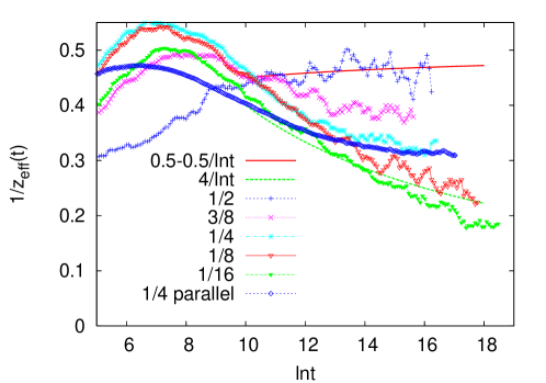
Figure 8: Effective dynamical exponents of coarsening in the bidirectional, two-lane model measured in Monte Carlo simulations at different global densities $N/2L=1/2,3/8,1/4,1/8,1/16$. Simulations have been perfomed with the random sequential update, except one of the data sets, which was obtained by the parallel update for $L=48000$ and $10^{2}$ samples.

As can be seen in the figure, at half-filling, the effective dynamical exponent seems to tend to $0.5$ but very slowly, possibly with a logarithmic correction. The solid curve fitting well to the data corresponds to the form $W(t)\sim(t/\ln t)^{1/2}$. Below half-filling, the effective exponent $1/z_{\rm eff}(t)$ is decreasing with $t$ for long times. For large enough densities, such as $3/8$ and $1/4$, it seems to tend to finite limiting values which decrease with the density. For smaller densities the effective exponents $1/z_{\rm eff}(t)$ decrease more quickly and from the data obtained at finite time scales it is difficult to decide whether they tend to finite values or to zero. The latter case may correspond to a logarithmic coarsening law $W(t)\sim[\ln(t/t_{0})]^{1/\psi}$ with some finite barrier exponent $\psi$. As a comparison, the dependence of the effective exponent $1/z_{\rm eff}(t)$ on time in this case with $\psi=0.25$ and $t_{0}=1$ is plotted in the figure.

4.4 The mean-field model

We have also studied the above model within the mean-field approximation. Here, one has the following evolution equations for the local densities $\rho_{i}(t)$ and $\pi_{i}(t)$ in lane A and B, respectively:

$$\frac{d\rho_{i}}{dt}=\rho_{i-1}(1-\rho_{i})-\rho_{i}(1-\rho_{i+1})+v_{i}\pi_{i}(1-\rho_{i})-u_{i}\rho_{i}(1-\pi_{i})$$

$$\frac{d\pi_{i}}{dt}=\pi_{i+1}(1-\pi_{i})-\pi_{i}(1-\pi_{i-1})-v_{i}\pi_{i}(1-\rho_{i})+u_{i}\rho_{i}(1-\pi_{i}),$$ (18)

for $i=1,2,\dots,L$. The steady state of the mean-field model is, however, much different from that of the original one, as can be seen from the steady state of the homogeneous model containing a reverse bias region. The mean-field treatment cannot describe the diffusive motion of the half-filled particle cluster mentioned in the previous section. Instead, the front of this cluster is pinned in the middle of the reverse bias region. This leads to an exponentially decreasing current with the length of the reverse bias region, and to Eq. (14) for the finite-size scaling of the current and to Eq. (15) for the coarsening dynamics in the disordered model. We have calculated the stationary current at a density $N/2L=1/4$ for different system sizes by solving Eqs. (18) in $10^{4}$ samples for each $L$. The distribution of the current shown in Fig. 9 indeed follows the law given in Eq. (14). In addition to this, we have followed the evolution of the surface width in large systems at the same density. The time dependence of the surface width averaged over a few samples is again in agreement with the prediction in Eq. (15), as can be seen in Fig. 9.

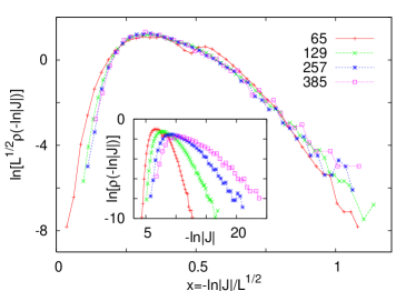
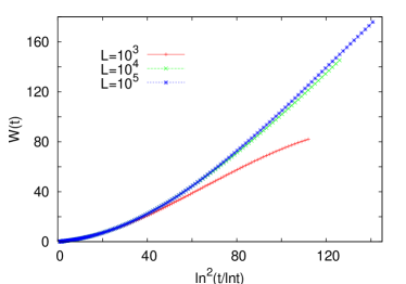
Figure 9: Left: Scaling plot of the distribution of the logarithm of the stationary current obtained for different sizes by the mean-field approximation. The unscaled data are shown in the inset. Right: Time-dependence of the surface width in the mean-field two-lane model.

5 Discussion

In this work, we have considered different exclusion processes, in which the disorder in the transition rates results in anomalous dynamics compared to the clean model. For the DTASEP, improving an earlier phenomenological model [12], we have obtained the form of logarithmic correction in the coarsening law, which is found to be compatible with results of Monte Carlo simulations. In the DPASEP, we have confirmed the earlier predicted logarithmically slow coarsening dynamics by numerical simulations.

Then we have studied a bidirectional, two-lane exclusion process with disordered lane-change rates, the dynamics of which are less known than in the case of the previous two models. In the absence of a potential, the steady state and the non-stationary behavior are non-trivial and are much different compared to those of the disordered partially asymmetric one-lane model. In the steady state, the disorder induces formation of particle and hole condensates of fluctuating size, which leads to anomalously large fluctuations of the equivalent surface. The fact that particle clusters accumulating at bottlenecks are delocalized makes possible a faster coarsening than in the DPASEP. Numerical simulations show that for particle densities not far from $1/2$, the coarsening is described by power-laws (apart from possible logarithmic corrections) with density-dependent dynamical exponents. For the particular case of the half-filled lattice, the dynamics are found to be characterized roughly by the exponents $\alpha=1$, $\beta=0.5$ and $z=2$, again with possible logarithmic corrections. For smaller densities, the inverse of the effective dynamical exponent seems to decrease constantly, but it is not possible to decide from the numerical data whether it tends to finite values.

The slowing of the dynamics with decreasing density is consistent with that the motion of a single particle is ultra-slow, characterized formally by an infinite dynamical exponent. Note, however, that approaching to the zero density through positive densities, i.e. performing $N/2L\to 0$ in an infinite system may give a limit dynamical law that is different from that of the single particle.

It is worth mentioning that even for densities close to $1/2$ the asymptotic region with a presumably finite dynamical exponent sets in only after a very long transient. In the transient, the coarsening, as well as the finite-size scaling of the stationary current (not shown) can be well described by an actived scaling with some effective barrier exponent $\psi$, that is smaller than $1/2$. Probing the dynamics of the model by finite-size scaling of the distribution of the stationary current is hard since, due to the long transient, large system sizes are needed and samples in the small-current tail of the distribution have extemely long relaxation times. The mean-field version of the above model, where particle clusters at bottlenecks are localized, shows logarithmically slow coarsening formally with an infinitely large dynamical exponent. So we can conclude, that the slow modes related to the delocalized particle clusters near barriers are important with respect to the dynamics of coarsening.

In Table 1, we have summarized the finite-size scaling behavior of the stationary current in disordered variants of the ASEP investigated here or earlier.

Table 1: Comparison of the finite-size scaling of the stationary current in the one-lane DPASEP and the bidirectional, two-lane model with disordered lane-change rates.

type of model	one-lane	two-lane
single barrier of length $l$	$J\sim e^{-cl}$	$J\sim 1/l$
biased ($F>0$)	$J\sim L^{-a(F)}$	$J\sim 1/\ln(L)$
unbiased ($F=0$)	$-\ln|J|\sim L^{1/2}$	density dependent

Interesting extensions of these investigations would be the study of dynamics in multi-lane transport systems or in the disordered ASEP in higher dimensions [39].

6 Acknowledgments

This paper was supported by the János Bolyai Research Scholarship of the Hungarian Academy of Sciences (RJ), by the Hungarian National Research Fund OTKA under grant nos. T77629, K75324, and by the bilateral German-Hungarian exchange program DAAD-MÖB under grant nos. 50450744, P-MÖB/854. The authors thank NVIDIA for supporting the project with high-performance graphics cards within the framework of Professor Partnership.

Appendix A

We have performed the Monte Carlo simulations with parallel updates according to the following scheme. In the case of the DTASEP, we used a parallel two-sub-lattice update shown in Fig. 10. Here, the lattice is divided into even and odd sub-lattices, which are updated alternately. In the case of the DPASEP, a similar two-sub-lattice update has been applied as given above.

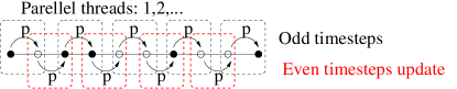
Figure 10: Illustration of the parallel, two-sub-lattice update applied for the DTASEP

In the case of the bidirectional, two-lane model with parallel update each Monte Carlo step consists of the following operations: (i) even sub-lattice updates of the lanes $A$ and $B$, with probabilities $1/2$, (ii) lane changes with probabilities $u_{i}$ and $v_{i}$, (iii) odd sub-lattice updates of the lanes $A$ and $B$ with probabilities $1/2$, (iv) lane changes with probabilities $u_{i}$ and $v_{i}$. Further details can be found in Ref. [23].

References

References

- [1] Chowdhury D, Santen L, and Schadschneider A 2000 Phys. Rep. 329 199
- [2] Konzack S, Rischitor P E, Enke C and Fischer R 2005 Mol. Biol. Cell 16 497; Nishinari K, Okada Y, Schadschneider A and Chowdhury D 2005 Phys. Rev. Lett. 95 118101; Greulich P, Garai A, Nishinari K, Schadschneider A and Chowdhury D 2007 Phys. Rev. E 75 041905
- [3] MacDonald C T, Gibbs J H and Pipkin A C 1968 Biopolymers 6 1
- [4] Spitzer F 1970 Adv. Math. 5 246
- [5] Liggett T M 1999 Stochastic interacting systems: contact, voter, and exclusion processes (Berlin, Springer)
- [6] Schütz G M 2001 in Phase Transitions and Critical Phenomena, vol. 19, edited by Domb C and Lebowitz J L (Academic, San Diego)
- [7] Ramaswamy R, Barma M 1987 J. Phys. A: Math. Gen. 20 2973
- [8] Koscielny-Bunde E, Bunde A, Havlin S, and Stanley H E 1988 Phys. Rev. A 37 1821
- [9] Tripathy G, Barma M 1997 Phys. Rev. Lett. 78 3039; 1998 Phys. Rev. E 58 1911
- [10] Goldstein S, Speer E R 1998 Phys. Rev. E 58 4226
- [11] Kolwankar K M, Punnoose A 2000 Phys. Rev. E 61 2453
- [12] Krug J, 2000 Braz. J. Phys. 30 97
- [13] Harris R J, Stinchcombe R B 2004 Phys. Rev. E 70 016108
- [14] Juhász R, Santen L and Iglói F 2005 Phys. Rev. Lett. 94 010601; 2006 Phys. Rev. E 74 061101
- [15] Juhász R, Lin Y-C, Iglói F 2006 Phys. Rev. B 73 224206
- [16] Barma M 2006 Physica A 372 22
- [17] Greulich P, Schadschneider A 2008 J. Stat. Mech. P04009
- [18] Juhász R 2011 J. Stat. Mech. P11010
- [19] Plischke M, Rácz Z and Liu D 1987 Phys. Rev. B 35 3485
- [20] Kardar M, Parisi G and Zhang Y 1986 Phys. Rev. Lett. 56 889
- [21] Barabási A L and Stanley H E 1995 Fractal Concepts in Surface Growth Cambridge University Press, Cambridge
- [22] Ódor G 2008 Universality in Nonequilibrium Lattice Systems World Scientific; 2004 Rev. Mod. Phys. 76 663
- [23] Schulz Henrik, Ódor Géza, Ódor Gergely, Nagy F. Máté 2011 Comp. Phys. Comm. 182 1467
- [24] Preis T at al 2009 J. of Comp. Phys. 228 4468
- [25] Weigel M 2012 J. of Comp. Phys. 231 3064.
- [26] Bernaschi M, Parisi G, Parisi L arXiv:1006.2566v1
- [27] Juhász R 2010 J. Stat. Mech. P03010
- [28] Evans M R and Hanney T 2005 J. Phys. A: Math. Gen. 38 R195
- [29] Jain K and Barma M 2003 Phys. Rev. Lett. 91 135701
- [30] Krug J and Meakin P 1990 J. Phys. A: Math. Gen. 23 L987
- [31] Queiroz S L A and Stinchcombe R B 2008 Phys. Rev. E 78 031106
- [32] Bouchaud J P, Georges A 1990 Phys. Rep. 195 127
- [33] Sinai Ya.G. 1982 Theory Probab. Appl. 27 256
- [34] Juhász R 2007 Phys. Rev. E 76 021117
- [35] Gross S P 2004 Phys. Biol. 1 R1
- [36] Klumpp S and Lipowsky R 2005 Phys. Rev. Lett. 95 268102
- [37] Ashwin P, Lin C, Steinberg G 2010 Phys. Rev. E 82 051907
- [38] Edwards S F, Wilkinson D R 1982 Proc. R. Soc. 381 17
- [39] Ódor G, Liedke B, and Heinig K-H 2010 Phys. Rev. E 81 031112