Inversion of circular means and the wave equation
on convex planar domains

Abstract

We study the problem of recovering the initial data of the two dimensional wave equation from values of its solution on the boundary $\partial\Omega$ of a smooth convex bounded domain $\Omega\subset\mathbb{R}^{2}$. As a main result we establish back-projection type inversion formulas that recover any initial data with support in $\Omega$ modulo an explicitly computed smoothing integral operator $\mathcal{K}_{\Omega}$. For circular and elliptical domains the operator $\mathcal{K}_{\Omega}$ is shown to vanish identically and hence we establish exact inversion formulas of the back-projection type in these cases. Similar results are obtained for recovering a function from its mean values over circles with centers on $\partial\Omega$. Both reconstruction problems are, amongst others, essential for the hybrid imaging modalities photoacoustic and thermoacoustic tomography.

1 Introduction

Let $\Omega\subset\mathbb{R}^{2}$ be a convex bounded domain in the plane with smooth boundary $\partial\Omega$. Suppose that $f\colon\mathbb{R}^{2}\to\mathbb{R}$ is a smooth function that vanishes outside $\Omega$, and denote by $u\colon\mathbb{R}^{2}\times\left(0,\infty\right)\to\mathbb{R}$ the solution of the initial value problem

$$\left\{\begin{aligned} \left(\partial_{t}^{2}-\Delta_{x}\right)u\left(x,t\right)&=0&\text{ for }\left(x,t\right)\in\mathbb{R}^{2}\times\left(0,\infty\right)\\ u\left(x,0\right)&=f\left(x\right)&\text{ for }x\in\mathbb{R}^{2}\\ \left(\partial_{t}u\right)\left(x,0\right)&=0&\text{ for }x\in\mathbb{R}^{2}\end{aligned}\right.\,.$$ (1.1)

In this paper we study the problem of recovering the unknown initial data $f$ from the values of the solution $u$ on the observation surface $\partial\Omega\times\left(0,\infty\right)$. Because the solution of (1.1) can be expressed in terms of circular means (and vice versa), the inversion of the wave equation is basically equivalent to the problem of recovering the function $f$ from its averages over circles with centers on $\partial\Omega$. Both reconstruction problems are essential for the novel hybrid imaging methods photoacoustic tomography (PAT) and thermoacoustic tomography (TAT). The standard setups in PAT/TAT using point-like detectors require the inversion of the wave equation in three spatial dimensions [1, 2]. The two dimensional version considered in this paper arises in a variant of PAT/TAT that uses linear integrating detectors instead of point-like ones (see [3, 4]). Inversion of circular means and the wave equation is also relevant for other imaging modalities, such as SONAR [5] or ultrasound tomography [6].

In the recent years, many reconstruction techniques for the wave inversion and the inversion from circular means (or spherical means in higher dimensions) have been developed. These techniques can be classified in iterative reconstruction methods (see [4, 7, 8, 9, 10]), model based time reversal (see [11, 12, 13, 14]), Fourier domain algorithms (see [6, 15, 16, 17, 18, 19]), and algorithms based on explicit reconstruction formulas of the back-projection type (see [5, 12, 20, 21, 22, 23, 24, 25, 26, 27]). The back-projection approach is particularly appealing since it is theoretically exact, stable with respect to data and modeling imperfections, mathematically elegant, and quite straightforward to implement numerically. Until recently, however, exact back-projection type reconstruction formulas were only known for the cases where $\partial\Omega$ is a spherical, planar or cylindrical surface (in three spatial dimensions) and a circle or a line (in two spatial dimensions). Many researchers even believed that exact reconstruction formulas of the back-projection type exist only in such cases. Only very recently the so called universal back-projection formula (originally introduced to PAT/TAT in [27]) has been shown in [25] to provide theoretically exact reconstruction for ellipsoids in $\mathbb{R}^{3}$. In the same paper it has further be shown that for general convex domains in $\mathbb{R}^{3}$ the universal back-projection formula is exact modulo an explicitly given smoothing integral operator.

In this paper we establish back-projection type reconstruction formulas for the inversion of the two dimensional wave equation on convex domains $\Omega\subset\mathbb{R}^{2}$. As their counterparts in three spatial dimensions, the derived formulas provide exact reconstruction modulo an explicitly computed smoothing integral operator $\mathcal{K}_{\Omega}$. We further show that for elliptical and circular domains the operator $\mathcal{K}_{\Omega}$ vanishes and therefore we obtain exact back-projection type reconstruction formulas in these cases. The same type of results are derived for reconstructing a function from its mean values over circles with centers on the boundary of a convex domain in the plane. Note that our reconstruction formulas as well as the proofs differ from the ones given in [25]. This partially accounts for the fact that the three dimensional wave equation satisfies a strong form of Huygens principle, whereas the two dimensional wave equation does not.

1.1 Notation

Before presenting our main results we introduce some notation that will be used throughout this article.

For any $k\in\mathbb{N}\cup\left\{\infty\right\}$, we denote by $C_{c}^{k}\left(\Omega\right)$ the set of all $k$-times continuously differentiable functions $f\colon\mathbb{R}^{2}\to\mathbb{R}$ which have support in $\Omega$. For given $f\in C_{c}^{\infty}\left(\Omega\right)$ we denote by $\mathcal{U}f\colon\mathbb{R}^{2}\times\left(0,\infty\right)\to\mathbb{R}$ the solution of the wave equation (1.1) with initial data $f$. Further, for some integrable function $f\colon\mathbb{R}^{2}\to\mathbb{R}$, the circular mean transform $\mathcal{M}f\colon\mathbb{R}^{2}\times\left(0,\infty\right)\to\mathbb{R}$ is defined by

$$\left(\mathcal{M}f\right)\left(x,r\right):=\frac{1}{2\pi}\int_{S^{1}}f\left(x+r\omega\right)\mathrm{d}\omega\qquad\text{ for }\left(x,r\right)\in\mathbb{R}^{2}\times\left(0,\infty\right)\,.$$ (1.2)

Here and below $S^{1}:=\left\{x\in\mathbb{R}^{2}:\left|x\right|=1\right\}$ denotes the unit sphere in $\mathbb{R}^{2}$ with $\lvert x\rvert$ being the Euclidian norm of $x\in\mathbb{R}^{2}$. The corresponding inner product of two points $x_{0},x_{1}\in\mathbb{R}^{2}$ will be denoted by $x_{0}\cdot x_{1}$. Similarly, the (classical) Radon transform $\mathcal{R}f\colon S^{1}\times\mathbb{R}\to\mathbb{R}$ is defined by

$$\left(\mathcal{R}f\right)\left(n,a\right):=\int_{\mathbb{R}}f\left(an+bn^{\bot}\right)\mathrm{d}b\qquad\text{ for }\;\left(n,a\right)\in S^{1}\times\mathbb{R}\,,$$

where $n^{\bot}\in S^{1}$ denotes a unit vector orthogonal to $n$. The derivative of a function $\phi\colon S^{1}\times\mathbb{R}\to\mathbb{R}$ with respect to the second variable will be denoted by $\left(\partial_{a}\phi\right)\left(n,a\right)$, and $\left(\mathcal{H}_{a}\phi\right)\left(n,a\right)$ will be used to denote the Hilbert transform of $\phi$ in the second argument, defined as the distributional convolution with $1/(\pi a)$.

We further write $\chi_{\Omega}\colon\mathbb{R}^{2}\to\mathbb{R}$ for the characteristic function of the domain $\Omega$ (taking the value one inside $\Omega$ and zero outside) and set

$$\hat{n}\left(x_{1},x_{0}\right):=\frac{x_{1}-x_{0}}{\left|x_{1}-x_{0}\right|}\,,\;\;\hat{a}\left(x_{1},x_{0}\right):=\frac{1}{2}\;\frac{\left|x_{1}\right|^{2}-\left|x_{0}\right|^{2}}{\left|x_{1}-x_{0}\right|}\qquad\text{ for }\;x_{1}\neq x_{0}\in\mathbb{R}^{2}\,.$$ (1.3)

Finally, for any $f\in C_{c}^{\infty}\left(\Omega\right)$ and any $x_{0}\in\Omega$, we define

$$\left(\mathcal{K}_{\Omega}f\right)\left(x_{0}\right):=\frac{1}{8\pi}\int_{\Omega}f\left(x_{1}\right)\frac{\left(\partial_{a}^{2}\mathcal{H}_{a}\mathcal{R}\chi_{\Omega}\right)\left(\hat{n}\left(x_{1},x_{0}\right),\hat{a}\left(x_{1},x_{0}\right)\right)}{\left|x_{1}-x_{0}\right|}\,\mathrm{d}x_{1}\,.$$ (1.4)

It can be readily verified that the line $\ell\left(x_{1},x_{0}\right)=\{x\in\mathbb{R}^{2}:\hat{n}\left(x_{1},x_{0}\right)\cdot x=\hat{a}\left(x_{1},x_{0}\right)\}$ consists of all points having the same distance between $x_{0}$ and $x_{1}$; compare with Figure 1.1.

\psfrag{a}{\scriptsize$x_{0}$}\psfrag{b}{\scriptsize$x_{1}$}\psfrag{s}{\scriptsize$\hat{a}\left(x_{1},x_{0}\right)$}\psfrag{O}{\scriptsize domain $\Omega$}\psfrag{S}{\scriptsize boundary $\partial\Omega$}\psfrag{m}{\scriptsize$\left(x_{1}+x_{0}\right)/2$}\psfrag{E}{\scriptsize$\ell\left(x_{1},x_{0}\right)$}\includegraphics[width=216.81pt]{domain.eps}

Figure 1.1: Let $\ell\left(x_{1},x_{0}\right)$ denote the line of all points having the same distance between $x_{1}$ and $x_{0}$. Then $\hat{n}\left(x_{1},x_{0}\right)=(x_{1}-x_{0})/\lvert x_{1}-x_{0}\rvert$ is the normal vector to $\ell\left(x_{1},x_{0}\right)$ and $\hat{a}\left(x_{1},x_{0}\right)=(\lvert x_{1}\rvert^{2}-\lvert x_{0}\rvert^{2})/\left(2\lvert x_{1}-x_{0}\rvert\right)$ is the oriented distance of the line $\ell\left(x_{1},x_{0}\right)$ from the origin.

1.2 Main results

Our first pair of results states that a back-projection type inversion formula applied to the solution of the wave equation (1.1) recovers any initial data $f$ modulo the term $\mathcal{K}_{\Omega}f$.

Theorem 1.1 (Inversion of the wave equation).

Let $\Omega\subset\mathbb{R}^{2}$ be a convex bounded domain with smooth boundary $\partial\Omega$. Then, for every function $f\in C_{c}^{\infty}\left(\Omega\right)$ and every reconstruction point $x_{0}\in\Omega$, we have

$$f\left(x_{0}\right)-\left(\mathcal{K}_{\Omega}f\right)\left(x_{0}\right) =\frac{1}{\pi}\,\nabla_{x_{0}}\cdot\int_{\partial\Omega}\nu_{x}\left(\int_{\left|x-x_{0}\right|}^{\infty}\frac{\left(\mathcal{U}f\right)\left(x,t\right)}{\sqrt{t^{2}-\left|x-x_{0}\right|^{2}}}\,\mathrm{d}t\right)\mathrm{d}s\left(x\right)\,,$$ (1.5)

$$f\left(x_{0}\right)-\left(\mathcal{K}_{\Omega}f\right)\left(x_{0}\right) =\frac{1}{\pi}\,\int_{\partial\Omega}\nu_{x}\cdot\left(x_{0}-x\right)\left(\int_{\left|x-x_{0}\right|}^{\infty}\frac{\left(\partial_{t}t^{-1}\mathcal{U}f\right)\left(x,t\right)}{\sqrt{t^{2}-\left|x-x_{0}\right|^{2}}}\,\mathrm{d}t\right)\mathrm{d}s\left(x\right)\,.$$ (1.6)

Here $\mathcal{U}f$ is the solution of (1.1), $\mathcal{K}_{\Omega}f$ is defined by (1.4), $\mathrm{d}\ell$ is the usual arc length measure on $\partial\Omega$, $\nu_{x}$ denotes the outwards pointing unit normal to $\partial\Omega$, and $\nabla_{x_{0}}\cdot$ denotes the divergence with respect to $x_{0}$.

Proof.

See Section 3. ∎

We also prove the following corresponding formulas for recovering a function from its mean values over circles centered on the boundary $\partial\Omega$.

Theorem 1.2 (Inversion from circular means).

Let $\Omega\subset\mathbb{R}^{2}$ be a convex bounded domain with smooth boundary $\partial\Omega$. Then, for every $f\in C_{c}^{\infty}\left(\Omega\right)$ and every $x_{0}\in\Omega$, we have

$$f\left(x_{0}\right)-\left(\mathcal{K}_{\Omega}f\right)\left(x_{0}\right) =\frac{1}{\pi}\,\nabla_{x_{0}}\cdot\int_{\partial\Omega}\nu_{x}\left(\int_{0}^{\infty}\frac{r\left(\mathcal{M}f\right)\left(x,r\right)}{r^{2}-\left|x-x_{0}\right|^{2}}\,\mathrm{d}r\right)\mathrm{d}s\left(x\right)\,,$$ (1.7)

$$f\left(x_{0}\right)-\left(\mathcal{K}_{\Omega}f\right)\left(x_{0}\right) =\frac{1}{\pi}\,\int_{\partial\Omega}\nu_{x}\cdot\left(x_{0}-x\right)\left(\int_{0}^{\infty}\frac{\left(\partial_{r}\mathcal{M}f\right)\left(x,r\right)}{r^{2}-\left|x-x_{0}\right|^{2}}\,\mathrm{d}r\right)\mathrm{d}s\left(x\right)\,.$$ (1.8)

Here both inner integrals have to be taken in the principal value sense, $\mathcal{M}f$ is the circular mean transform defined by (1.2), and $\mathcal{K}_{\Omega}$, $\nu_{x}$, $\mathrm{d}\ell$ and $\nabla_{x_{0}}$ are as in Theorem 1.1.

Proof.

See Section 4. ∎

Remark 1.3 (Smoothing effect of $\mathcal{K}_{\Omega}$).

If $\Omega\subset\mathbb{R}^{2}$ is smooth and convex, then the Radon transform of $\chi_{\Omega}$ is smooth except for such pairs of $\left(n,a\right)\in S^{1}\times\mathbb{R}$ where the line $\left\{x\in\mathbb{R}^{2}:n\cdot x=a\right\}$ is tangential to the boundary $\partial\Omega$. Notice further, that for $x_{1}\neq x_{0}\in\Omega$ the line $\ell\left(x_{1},x_{0}\right)$ is never tangential to $\partial\Omega$; see Figure 1.1. Since the operator $\partial_{a}^{2}\mathcal{H}_{a}$ preserves the locations of the singularities of $\mathcal{R}\chi_{\Omega}$ this shows that the kernel in (1.4) has at most a weak singularity proportional to $1/\left|x_{1}-x_{0}\right|$ and hence is at least smoothing by one degree.

For special domains, the integral operator $\mathcal{K}_{\Omega}$ may vanish, in which cases Theorems 1.1 and 1.2 provide exact reconstruction formulas for the inversion of the wave equation and the inversion from circular means, respectively. We verify that this is indeed the case for circular and elliptical domains.

Theorem 1.4 (Exact inversion for circular and elliptical domains).

Let $\Omega\subset\mathbb{R}^{2}$ be a circular or elliptical domain and let $f\colon\mathbb{R}^{2}\to\mathbb{R}$ be a $C^{\infty}$ function with support in $\Omega$. Then $\mathcal{K}_{\Omega}f$ vanishes identically on $\Omega$. In particular, the following hold:

1. The function $f$ can be recovered from the solution of the wave equation (1.1) by means of either of the following formulas:

   $$f\left(x_{0}\right) =\frac{1}{\pi}\,\nabla_{x_{0}}\cdot\int_{\partial\Omega}\nu_{x}\left(\int_{\left|x-x_{0}\right|}^{\infty}\frac{\left(\mathcal{U}f\right)\left(x,t\right)}{\sqrt{t^{2}-\left|x-x_{0}\right|^{2}}}\,\mathrm{d}t\right)\mathrm{d}s\left(x\right)\,,$$ (1.9)

   $$f\left(x_{0}\right) =\frac{1}{\pi}\,\int_{\partial\Omega}\nu_{x}\cdot\left(x_{0}-x\right)\left(\int_{\left|x-x_{0}\right|}^{\infty}\frac{\left(\partial_{t}t^{-1}\mathcal{U}f\right)\left(x,t\right)}{\sqrt{t^{2}-\left|x-x_{0}\right|^{2}}}\,\mathrm{d}t\right)\mathrm{d}s\left(x\right)\,.$$ (1.10)

2. The function $f$ can be recovered from the circular averages $\mathcal{M}f$ defined in (1.2) by means of either of the following formulas:

   $$f\left(x_{0}\right) =\frac{1}{\pi}\,\nabla_{x_{0}}\cdot\int_{\partial\Omega}\nu_{x}\left(\int_{0}^{\infty}\frac{r\left(\mathcal{M}f\right)\left(x,r\right)}{r^{2}-\left|x-x_{0}\right|^{2}}\,\mathrm{d}r\right)\mathrm{d}s\left(x\right)\,,$$ (1.11)

   $$f\left(x_{0}\right) =\frac{1}{\pi}\,\int_{\partial\Omega}\nu_{x}\cdot\left(x_{0}-x\right)\left(\int_{0}^{\infty}\frac{\left(\partial_{r}\mathcal{M}f\right)\left(x,r\right)}{r^{2}-\left|x-x_{0}\right|^{2}}\,\mathrm{d}r\right)\mathrm{d}s\left(x\right)\,.$$ (1.12)

   Here both inner integrals have to be taken in the principal value sense.

Proof.

See Section 5. ∎

1.3 Prior work and innovations

In the case that $\Omega$ is a spherical domain in $d\geq 2$ dimension, various exact back-projection type inversion formulas for the inversion of the wave equation and the inversion from spherical means have been derived in [3, 12, 21, 23, 27]. In particular, the inversion formula [3] coincides with our formula (1.10) for the wave inversion, and the formula of [23] for the inversion from circular means (if rewritten as in [28]; see [29] for a different derivation) coincides with our formula (1.11). However, in [3, 23] these formulas are neither shown be exact for elliptical domains, nor are they investigated for more general domains.

Inversion formulas for the spherical mean transform on elliptical domains have been derived recently in [26]. The methods and results there are different from ours and no statements are made for general convex domains. Even the reconstruction formula of [26] for ellipses differs from each of our formulas (1.11), (1.12). Our results are more closely related to the one of [25], where corresponding results have derived for convex domains in $\mathbb{R}^{3}$. Note further that in three spatial dimensions a statement similar to our Theorem 1.1 is also present in [27] (where, however, no explicit expression for the operator $\mathcal{K}_{\Omega}$ has been derived). Anyway, none of the papers [25, 27] considers the two-dimensional case.

1.4 Outline

The following sections are devoted to the proofs of the theorems presented in Section 1.2. In Section 2 we derive auxiliary statements that we require for the proofs of these results. In Section 3 we then derive the formulas for the wave inversion claimed in Theorem 1.1 and in Section 4 we establish the corresponding results for the inversion from circular means. The cases of circular and elliptical domains are considered in Section 5, where we show that the operator $\mathcal{K}_{\Omega}$ vanishes in these cases and hence we establish the exact inversion formulas claimed in Theorem 1.4. The paper concludes with a short discussion in Section 6.

2 Auxiliary results

For the following considerations recall the definitions of the circular mean transform $\mathcal{M}$, the Radon transform $\mathcal{R}$, and the operator $\mathcal{U}$ that maps any initial data $f\in C_{c}^{\infty}\left(\Omega\right)$ to the solution of (1.1); see Section 1.1. We will further make use of the operator $\mathcal{V}$, which maps any $f\in C_{c}^{\infty}\left(\Omega\right)$ to the solution $v\colon\mathbb{R}^{2}\times\left(0,\infty\right)\to\mathbb{R}$ of the initial value problem

$$\left\{\begin{aligned} \left(\partial_{t}^{2}-\Delta_{x}\right)v\left(x,t\right)&=0&\text{ for }\left(x,t\right)\in\mathbb{R}^{2}\times\left(0,\infty\right)\\ v\left(x,0\right)&=0&\text{ for }x\in\mathbb{R}^{2}\\ \left(\partial_{t}v\right)\left(x,0\right)&=f\left(x\right)&\text{ for }x\in\mathbb{R}^{2}\end{aligned}\;.\right.$$ (2.1)

One easily recognizes that $\mathcal{U}$ and $\mathcal{V}$ are related by the identity $\mathcal{U}f=\partial_{t}\mathcal{V}f$. Indeed, if $v$ solves (2.1), then by definition $u=\partial_{t}v$ satisfies the wave equation $(\partial_{t}^{2}-\Delta_{x})u=0$ and the initial condition $u\left(x,0\right)=f\left(0\right)$. Further, the wave equation yields $(\partial_{t}u)\left(x,0\right)=(\partial_{t}^{2}v)\left(x,0\right)=\left(\Delta_{x}v\right)\left(x,0\right)=0$ which shows that $u$ is a solution of (1.1).

Next we proof a simple integral identity that we require for the following considerations.

Lemma 2.1.

Suppose that $f\in C_{c}^{\infty}\left(\Omega\right)$ and that $\phi\colon\mathbb{R}^{2}\to\mathbb{R}$ is continuously differentiable on $\bar{\Omega}$ and vanishes outside $\bar{\Omega}$. Then, for every $x_{1}\in\Omega$, we have

$$\int_{\mathbb{R}^{2}}\phi\left(x\right)\left(\int_{0}^{\infty}\left(\partial_{r_{0}}\mathcal{M}f\right)\left(x,r_{0}\right)\ln\left|r_{0}^{2}-\left|x-x_{1}\right|^{2}\right|\mathrm{d}r_{0}\right)\mathrm{d}x\\ =\frac{1}{2\pi}\int_{\mathbb{R}^{2}}\frac{f\left(x_{0}\right)}{\left|x_{1}-x_{0}\right|}\left(\int_{\mathbb{R}}\left(\partial_{a}\mathcal{R}\phi\right)\left(\hat{n},a\right)\ln\left|2\left|x_{1}-x_{0}\right|\left(a-\hat{a}\right)\right|\mathrm{d}a\right)\mathrm{d}x_{0}\,.$$ (2.2)

Here $\hat{n}=\hat{n}\left(x_{1},x_{0}\right)$ and $\hat{a}=\hat{a}\left(x_{1},x_{0}\right)$ are defined by Equation (1.3).

Proof.

We first verify (2.2) with $\Phi\left(\,\cdot\,\right)$ in place of $\ln\left|\,\cdot\,\right|$, where $\Phi\colon\mathbb{R}\to\mathbb{R}$ is continuously differentiable and integrable. Hence we show that for every $x_{1}\in\Omega$ the following holds:

$$\int_{\mathbb{R}^{2}}\phi\left(x\right)\left(\int_{0}^{\infty}\left(\partial_{r_{0}}\mathcal{M}f\right)\left(x,r_{0}\right)\Phi\left(r_{0}^{2}-\left|x-x_{1}\right|^{2}\right)\mathrm{d}r_{0}\right)\mathrm{d}x\\ =\frac{1}{2\pi}\int_{\mathbb{R}^{2}}\frac{f\left(x_{0}\right)}{\left|x_{1}-x_{0}\right|}\left(\int_{\mathbb{R}}\left(\partial_{a}\mathcal{R}\phi\right)\left(\hat{n},a\right)\Phi\left(2\left|x_{1}-x_{0}\right|\left(a-\hat{a}\right)\right)\mathrm{d}a\right)\mathrm{d}x_{0}\,.$$ (2.3)

After performing one integration by parts, using the definition of the circular mean transform, and introducing polar coordinates around the center $x$ afterwards, the inner integral on the left hand side of (2.3) can be written as

$$\int_{0}^{\infty}\left(\partial_{r_{0}}\mathcal{M}f\right)\left(x,r_{0}\right)\Phi\left(r_{0}^{2}-\left|x-x_{1}\right|^{2}\right)\mathrm{d}r_{0} =-2\int_{0}^{\infty}r_{0}\left(\mathcal{M}f\right)\left(x,r_{0}\right)\Phi^{\prime}\left(r_{0}^{2}-\left|x-x_{1}\right|^{2}\right)\mathrm{d}r_{0}$$

$$=-\frac{1}{\pi}\int_{0}^{\infty}\int_{S^{1}}r_{0}f\left(x+r_{0}\omega_{0}\right)\Phi^{\prime}\left(r_{0}^{2}-\left|x-x_{1}\right|^{2}\right)\mathrm{d}\omega_{0}\mathrm{d}r_{0}$$

$$=-\frac{1}{\pi}\int_{\Omega}f\left(x_{0}\right)\Phi^{\prime}\left(\left|x-x_{0}\right|^{2}-\left|x-x_{1}\right|^{2}\right)\mathrm{d}x_{0}\,.$$

By straight forward computation one verifies that $\left|x-x_{0}\right|^{2}-\left|x-x_{1}\right|^{2}=2\left(x_{1}-x_{0}\right)\cdot\left(x-\left(x_{1}+x_{0}\right)/2\right)$. Therefore, one application of Fubini’s theorem, the definition of the Radon transform and the definitions of $\hat{n}=\hat{n}\left(x_{1},x_{0}\right)$ and $\hat{a}=\hat{a}\left(x_{1},x_{0}\right)$ yield

$$\int_{\mathbb{R}^{2}}\phi\left(x\right)\int_{0}^{\infty}\left(\partial_{r_{0}}\mathcal{M}f\right)\left(x,r_{0}\right)\Phi\left(r_{0}^{2}-\left|x-x_{1}\right|^{2}\right)\mathrm{d}r_{0}\mathrm{d}x\\ \begin{aligned} &=-\frac{1}{\pi}\int_{\Omega}f\left(x_{0}\right)\int_{\mathbb{R}^{2}}\phi\left(x\right)\Phi^{\prime}\left(2\left(x_{1}-x_{0}\right)\cdot\left(x-\left(x_{1}-x_{0}\right)/2\right)\right)\mathrm{d}x\mathrm{d}x_{0}\\ &=-\frac{1}{\pi}\int_{\Omega}f\left(x_{0}\right)\left(\int_{\mathbb{R}}\int_{\mathbb{R}}\phi\left(a\hat{n}+b\hat{n}^{\bot}\right)\Phi^{\prime}\left(2\left|x_{1}-x_{0}\right|\left(a-\hat{a}\right)\right)\mathrm{d}b\mathrm{d}a\right)\mathrm{d}x_{0}\\ &=-\frac{1}{\pi}\int_{\Omega}f\left(x_{0}\right)\left(\int_{\mathbb{R}}\left(\mathcal{R}\phi\right)\left(\hat{n},a\right)\Phi^{\prime}\left(2\left|x_{1}-x_{0}\right|\left(a-\hat{a}\right)\right)\mathrm{d}a\right)\mathrm{d}x_{0}\end{aligned}$$

Finally, after performing one further integration by parts in the inner integral, the last expression is seen to be equal to

$$\frac{1}{2\pi}\int_{\Omega}\frac{f\left(x_{0}\right)}{\left|x_{1}-x_{0}\right|}\left(\int_{\mathbb{R}}\left(\partial_{a}\mathcal{R}\phi\right)\left(\hat{n},a\right)\Phi\left(2\left|x_{1}-x_{0}\right|\left(a-\hat{a}\right)\right)\mathrm{d}a\right)\mathrm{d}x_{0}\,.$$

This shows that (2.3) indeed holds for all $\Phi\in C^{1}\left(\mathbb{R}\right)\cap L^{1}\left(\mathbb{R}\right)$. In order to verify the corresponding identity for $\ln\left|\,\cdot\,\right|$ in place of $\Phi$ we may write $\ln\left|\,\cdot\,\right|$ as the $L^{1}$-limit of continuously differentiable functions $\Phi_{n}$. Application of (2.3) with $\Phi_{n}$ in place of $\Phi$ and taking the limit $n\to\infty$ afterwards then implies the desired identity (2.2). ∎

The next Lemma is the key for the results in this paper.

Lemma 2.2.

For all $f,g\in C_{c}^{\infty}\left(\Omega\right)$ we have

$$\int_{\Omega}\left(\int_{0}^{\infty}\left(\mathcal{U}f\right)\left(x,t\right)\left(\mathcal{V}g\right)\left(x,t\right)\,\mathrm{d}t\right)\mathrm{d}x\\ =-\frac{1}{8\pi}\int_{\Omega}\int_{\Omega}f\left(x_{0}\right)g\left(x_{1}\right)\frac{\left(\mathcal{H}_{a}\mathcal{R}\chi_{\Omega}\right)\left(\hat{n}\left(x_{1},x_{0}\right),\hat{a}\left(x_{1},x_{0}\right)\right)}{\left|x_{1}-x_{0}\right|}\,\mathrm{d}x_{0}\mathrm{d}x_{1}\,.$$ (2.4)

Here $\mathcal{H}_{a}$ is the Hilbert transform in the second argument, $\chi_{\Omega}$ is the characteristic function of $\Omega$, and $\hat{n}=\hat{n}\left(x_{1},x_{0}\right)$ and $\hat{a}=\hat{a}\left(x_{1},x_{0}\right)$ are defined by Equation (1.3).

Proof.

First recall that the explicit expressions for the solutions of the initial value problems (2.1) and (1.1) (see, for example, [30, p. 134]) are given by

$$\left(\mathcal{V}g\right)\left(x,t\right) =\int_{0}^{t}\frac{r\left(\mathcal{M}g\right)\left(x,r\right)}{\sqrt{t^{2}-r^{2}}}\,\mathrm{d}r\,,$$

$$\left(\mathcal{U}f\right)\left(x,t\right) =\partial_{t}\int_{0}^{t}\frac{r\left(\mathcal{M}f\right)\left(x,r\right)}{\sqrt{t^{2}-r^{2}}}\,\mathrm{d}r\,.$$

After performing one integration by parts and differentiating under the integral sign, the expression for $\mathcal{U}f$ can be rewritten as

$$\left(\mathcal{U}f\right)\left(x,t\right)=\partial_{t}\int_{0}^{t}\left(\partial_{r}\mathcal{M}f\right)\left(x,r\right)\sqrt{t^{2}-r^{2}}\,\mathrm{d}r\\ =\int_{0}^{t}\left(\partial_{r}\mathcal{M}f\right)\left(x,r\right)\frac{t}{\sqrt{t^{2}-r^{2}}}\,\mathrm{d}r\,.$$ (2.5)

These identities and Fubini’s theorem yield

$$\int_{0}^{\infty}\left(\mathcal{U}f\right)\left(x,t\right)\left(\mathcal{V}g\right)\left(x,t\right)\mathrm{d}t\\ \begin{aligned} &=\lim_{T\to\infty}\int_{0}^{T}t\left(\int_{0}^{t}\frac{\left(\partial_{r_{0}}\mathcal{M}f\right)\left(x,r_{0}\right)}{\sqrt{t^{2}-r_{0}^{2}}}\mathrm{d}r_{0}\right)\left(\int_{0}^{t}\frac{\left(r_{1}\mathcal{M}g\right)\left(x,r_{1}\right)}{\sqrt{t^{2}-r_{1}^{2}}}\mathrm{d}r_{1}\right)\mathrm{d}t\\ &=\lim_{T\to\infty}\int_{0}^{\infty}\left(r_{1}\mathcal{M}g\right)\left(x,r_{1}\right)\int_{0}^{\infty}\left(\partial_{r_{0}}\mathcal{M}f\right)\left(x,r_{0}\right)\left(\int_{\max\left\{r_{0},r_{1}\right\}}^{T}\frac{t\mathrm{d}t}{\sqrt{t^{2}-r_{0}^{2}}\sqrt{t^{2}-r_{1}^{2}}}\right)\mathrm{d}r_{0}\mathrm{d}r_{1}\,.\end{aligned}$$

The inner integral in the above expression evaluates to

$$\int_{\max\left\{r_{0},r_{1}\right\}}^{T}\frac{t\,\mathrm{d}t}{\sqrt{t^{2}-r_{1}^{2}}\sqrt{t^{2}-r_{0}^{2}}}\\ =\ln\left(\sqrt{T^{2}-r_{0}^{2}}+\sqrt{T^{2}-r_{1}^{2}}\right)-\frac{1}{2}\ln\left(\left|r_{0}^{2}-r_{1}^{2}\right|\right)\,.$$ (2.6)

Hence we obtain

$$\int_{0}^{\infty}\left(\mathcal{U}f\right)\left(x,t\right)\left(\mathcal{V}g\right)\left(x,t\right)\mathrm{d}t\\ \begin{aligned} &=\lim_{T\to\infty}\int_{0}^{\infty}\int_{0}^{\infty}\left(\partial_{r_{0}}\mathcal{M}f\right)\left(x,r_{0}\right)\left(r_{1}\mathcal{M}g\right)\left(x,r_{1}\right)\ln\left(\sqrt{T^{2}-r_{0}^{2}}+\sqrt{T^{2}-r_{1}^{2}}\right)\mathrm{d}r_{0}\mathrm{d}r_{1}\\ &\hskip 28.45274pt-\frac{1}{2}\int_{0}^{\infty}\int_{0}^{\infty}\left(\partial_{r_{0}}\mathcal{M}f\right)\left(x,r_{0}\right)\left(r_{1}\mathcal{M}g\right)\left(x,r_{1}\right)\ln\left|r_{0}^{2}-r_{1}^{2}\right|\mathrm{d}r_{0}\mathrm{d}r_{1}\,.\end{aligned}$$

After one integration by parts and performing the limit $T\to\infty$ afterwards, the first term on the right hand side is seen to vanish. Therefore, by integrating over the variable $x$, interchanging the order of integration and introducing polar coordinates, we obtain

$$\int_{\Omega}\int_{0}^{\infty}\left(\mathcal{U}f\right)\left(x,t\right)\left(\mathcal{V}g\right)\left(x,t\right)\mathrm{d}t\mathrm{d}x\\ =-\frac{1}{4\pi}\int_{\Omega}g\left(x_{1}\right)\left(\int_{\mathbb{R}^{2}}\chi_{\Omega}\left(x\right)\int_{0}^{\infty}\left(\partial_{r_{0}}\mathcal{M}f\right)\left(x,r_{0}\right)\ln\left|r_{0}^{2}-\left|x-x_{1}\right|^{2}\right|\mathrm{d}r_{0}\mathrm{d}x\right)\mathrm{d}x_{1}\,.$$

According to Lemma 2.1, the double integral in brackets equals

$$\frac{1}{2\pi}\int_{\Omega}\frac{f\left(x_{0}\right)}{\left|x_{1}-x_{0}\right|}\left(\int_{\mathbb{R}}\left(\partial_{a}\mathcal{R}\chi_{\Omega}\right)\left(\hat{n},a\right)\ln\left|2\left|x_{1}-x_{0}\right|\left(a-\hat{a}\right)\right|\mathrm{d}a\right)\mathrm{d}x_{0}\,.$$

Next note that the distributional derivative of $\ln\left|a\right|$ is $\mathrm{P.V.}\frac{1}{a}$. After recalling the definition of the Hilbert transform we therefore obtain

$$\int_{\Omega}\int_{0}^{\infty}\left(\mathcal{U}f\right)\left(x,t\right)\left(\mathcal{V}g\right)\left(x,t\right)\mathrm{d}t\mathrm{d}x\\ \begin{aligned} &=-\frac{1}{8\pi^{2}}\int_{\Omega}\int_{\Omega}\frac{f\left(x_{0}\right)g\left(x_{1}\right)}{\left|x_{1}-x_{0}\right|}\left(\int_{\mathbb{R}}\left(\partial_{a}\mathcal{R}\chi_{\Omega}\right)\left(\hat{n},a\right)\ln\left|2\left|x_{1}-x_{0}\right|\left(a-\hat{a}\right)\right|\mathrm{d}a\right)\mathrm{d}x_{0}\,\mathrm{d}x_{1}\\ &=-\frac{1}{8\pi^{2}}\int_{\Omega}\int_{\Omega}\frac{f\left(x_{0}\right)g\left(x_{1}\right)}{\left|x_{1}-x_{0}\right|}\left(\mathrm{P.V.}\int_{\mathbb{R}}\left(\mathcal{R}\chi_{\Omega}\right)\left(\hat{n},a\right)\frac{\mathrm{d}a}{\hat{a}-a}\right)\mathrm{d}x_{0}\,\mathrm{d}x_{1}\\ &=-\frac{1}{8\pi}\int_{\Omega}\int_{\Omega}\frac{f\left(x_{0}\right)g\left(x_{1}\right)}{\left|x_{1}-x_{0}\right|}\left(\mathcal{H}_{a}\mathcal{R}\chi_{\Omega}\right)\left(\hat{n},\hat{a}\right)\,\mathrm{d}x_{0}\mathrm{d}x_{1}\,.\end{aligned}$$

Hence we have verified (2.4) which concludes the proof ∎

We are now ready to derive the following auxiliary theorem from which we will extract all formulas presented in the introduction.

Theorem 2.3.

For all $f,g\in C_{c}^{\infty}\left(\Omega\right)$ we have

$$-2\int_{\partial\Omega}\nu_{x}\cdot\left(\int_{0}^{\infty}\left(\mathcal{U}f\right)\left(x,t\right)\left(\nabla_{x}\mathcal{V}g\right)\left(x,t\right)\mathrm{d}t\right)\mathrm{d}s\left(x\right)\\ =\int_{\Omega}f\left(x_{0}\right)g\left(x_{0}\right)\mathrm{d}x_{0}-\int_{\Omega}\left(\mathcal{K}_{\Omega}f\right)\left(x_{0}\right)g\left(x_{0}\right)\mathrm{d}x_{0}\,.$$ (2.7)

Here $\mathcal{U}$ and $\mathcal{V}$ denote the solution operators of the initial value problems (1.1) and (2.1), respectively, $\mathcal{K}_{\Omega}f$ is defined by (1.4), and $\nu_{x}$ denotes the outward pointing unit normal to $\partial\Omega$.

Proof.

Application of Greens second identity to the functions $\left(\mathcal{U}f\right)\left(\,\cdot\,,t\right)$ and $\left(\mathcal{V}g\right)\left(\,\cdot\,,t\right)$ with fixed $t$ followed by an integration over the temporal variable yields

$$\int_{0}^{\infty}\left(\int_{\Omega}\left(\left(\mathcal{V}g\right)\left(x,t\right)\left(\Delta_{x}\mathcal{U}f\right)\left(x,t\right)-\left(\mathcal{U}f\right)\left(x,t\right)\left(\Delta_{x}\mathcal{V}g\right)\left(x,t\right)\right)\mathrm{d}x\right)\mathrm{d}t\\ =\int_{0}^{\infty}\left(\int_{\partial\Omega}\nu_{x}\left(\left(\mathcal{V}g\right)\left(x,t\right)\left(\nabla_{x}\mathcal{U}f\right)\left(x,t\right)-\left(\mathcal{U}f\right)\left(x,t\right)\left(\nabla_{x}\mathcal{V}g\right)\left(x,t\right)\right)\mathrm{d}s\left(x\right)\right)\mathrm{d}t\,.$$

Since $\mathcal{V}f$ and $\mathcal{U}g$ are both solutions of the wave equation we have the equalities $\Delta_{x}\mathcal{U}f=\partial_{t}^{2}\mathcal{U}f$ and $\Delta_{x}\mathcal{V}g=\partial_{t}^{2}\mathcal{V}g$. Together with the relation $\left(\mathcal{V}g\right)\left(\nabla_{x}\mathcal{U}f\right)=\nabla_{x}\left(\mathcal{V}g\mathcal{U}f\right)-\left(\nabla_{x}\mathcal{V}g\right)\left(\mathcal{U}f\right)$ and one application of the divergence theorem this further implies

$$\int_{\Omega}\left(\int_{0}^{\infty}\left(\left(\mathcal{V}g\right)\left(x,t\right)\left(\partial_{t}^{2}\mathcal{U}f\right)\left(x,t\right)-\left(\mathcal{U}f\right)\left(x,t\right)\left(\partial_{t}^{2}\mathcal{V}g\right)\left(x,t\right)\right)\mathrm{d}t\right)\mathrm{d}x\\ =\int_{0}^{\infty}\left(\int_{\Omega}\Delta_{x}\left(\left(\mathcal{V}g\right)\left(x,t\right)\left(\mathcal{U}f\right)\left(x,t\right)\right)\mathrm{d}x\right)\mathrm{d}t-2\int_{0}^{\infty}\left(\int_{\partial\Omega}\nu_{x}\left(\left(\mathcal{U}f\right)\left(x,t\right)\left(\nabla_{x}\mathcal{V}g\right)\left(x,t\right)\right)\mathrm{d}s\left(x\right)\right)\mathrm{d}t\,.$$

After integrating the inner integrals on the right hand side by parts and using the initial conditions $\left(\mathcal{U}f\right)\left(\,\cdot\,,0\right)=f$, $\left(\partial_{t}\mathcal{U}f\right)\left(\,\cdot\,,0\right)=0$ and $\left(\partial_{t}\mathcal{V}g\right)\left(\,\cdot\,,0\right)=g$, the expression on the left hand side evaluates to $\int_{\Omega}f\left(x_{0}\right)g\left(x_{0}\right)\mathrm{d}x_{0}$ which yields

$$\int_{\Omega}f\left(x_{0}\right)g\left(x_{0}\right)\mathrm{d}x_{0}=\int_{\Omega}\int_{0}^{\infty}\Delta_{x}\left(\left(\mathcal{U}f\right)\left(x,t\right)\left(\mathcal{V}g\right)\left(x,t\right)\right)\mathrm{d}t\mathrm{d}x\\ -2\int_{\partial\Omega}\nu_{x}\int_{0}^{\infty}\left(\mathcal{U}f\right)\left(x,t\right)\left(\nabla_{x}\mathcal{V}g\right)\left(x,t\right)\mathrm{d}t\mathrm{d}s\left(x\right)\,.$$ (2.8)

Next notice that

$$\Delta_{x}\left(\left(\mathcal{U}f\right)\left(\mathcal{V}g\right)\right) =\left(\Delta_{x}\mathcal{U}f\right)\left(\mathcal{V}g\right)+2\left(\nabla_{x}\mathcal{V}f\right)\cdot\left(\nabla_{x}\mathcal{U}g\right)+\left(\mathcal{U}f\right)\left(\Delta_{x}\mathcal{V}g\right)$$

$$=\left(\mathcal{U}\Delta_{x}f\right)\left(\mathcal{V}g\right)+2\left(\mathcal{V}\nabla_{x}f\right)\cdot\left(\mathcal{U}\nabla_{x}g\right)+\left(\mathcal{U}f\right)\left(\mathcal{V}\Delta_{x}g\right)\,,$$

where $\mathcal{V}\nabla_{x}f$ (and similarly $\mathcal{U}\nabla_{x}g$) is defined by component-wise application of $\mathcal{V}$ to $\nabla_{x}f$. Hence in view of Lemma 2.2 and by repeated application of the divergence theorem we obtain

$$\int_{\Omega}\int_{0}^{\infty}\Delta_{x}\left(\left(\mathcal{U}f\right)\left(x,t\right)\left(\mathcal{V}g\right)\left(x,t\right)\right)\mathrm{d}t\mathrm{d}x\\ \begin{aligned} =&-\frac{1}{8\pi}\int_{\Omega}\int_{\Omega}\left(\nabla_{x_{0}}+\nabla_{x_{1}}\right)^{2}\left(f\left(x_{0}\right)g\left(x_{1}\right)\right)\frac{\left(\mathcal{H}_{a}\mathcal{R}\chi_{\Omega}\right)\left(\hat{n}\left(x_{1},x_{0}\right),\hat{a}\left(x_{1},x_{0}\right)\right)}{\left|x_{1}-x_{0}\right|}\,\mathrm{d}x_{0}\mathrm{d}x_{1}\\ =&-\frac{1}{8\pi}\int_{\Omega}\int_{\Omega}f\left(x_{0}\right)g\left(x_{1}\right)\left(\nabla_{x_{0}}+\nabla_{x_{1}}\right)^{2}\left(\frac{\left(\mathcal{H}_{a}\mathcal{R}\chi_{\Omega}\right)\left(\hat{n}\left(x_{1},x_{0}\right),\hat{a}\left(x_{1},x_{0}\right)\right)}{\left|x_{1}-x_{0}\right|}\right)\,\mathrm{d}x_{0}\mathrm{d}x_{1}\,.\end{aligned}$$

As easily verified, the following relations hold true:

$$\left(\nabla_{x_{1}}+\nabla_{x_{0}}\right)\hat{n}\left(x_{1},x_{0}\right)=0\,,$$

$$\left(\nabla_{x_{1}}+\nabla_{x_{0}}\right)\hat{a}\left(x_{1},x_{0}\right)=\left(x_{1}-x_{0}\right)/\left|x_{1}-x_{0}\right|\,,$$

$$\left(\nabla_{x_{1}}+\nabla_{x_{0}}\right)\left|x_{1}-x_{0}\right|^{-1}=0\,,$$

$$\left(\nabla_{x_{1}}+\nabla_{x_{0}}\right)\cdot\left(x_{1}-x_{0}\right)=0\,.$$

These relations imply

$$\left(\nabla_{x_{1}}+\nabla_{x_{0}}\right)^{2}\frac{\left(\mathcal{H}_{a}\mathcal{R}\chi_{\Omega}\right)\left(\hat{n},\hat{a}\right)}{8\pi\left|x_{1}-x_{0}\right|}=\left(\nabla_{x_{1}}+\nabla_{x_{0}}\right)\frac{x_{1}-x_{0}}{8\pi\left|x_{1}-x_{0}\right|^{2}}\left(\partial_{a}\mathcal{H}_{a}\mathcal{R}\chi_{\Omega}\right)\left(\hat{n},\hat{a}\right)=\frac{\left(\partial_{a}^{2}\mathcal{H}_{a}\mathcal{R}\chi_{\Omega}\right)\left(\hat{n},\hat{a}\right)}{8\pi\left|x_{1}-x_{0}\right|}\,,$$

and therefore

$$\int_{\Omega}\int_{0}^{\infty}\Delta_{x}\left(\left(\mathcal{U}f\right)\left(x,t\right)\left(\mathcal{V}g\right)\left(x,t\right)\right)\mathrm{d}t\mathrm{d}x\\ =-\frac{1}{8\pi}\int_{\Omega}\int_{\Omega}f\left(x_{0}\right)g\left(x_{1}\right)\frac{\left(\partial_{a}^{2}\mathcal{H}_{a}\mathcal{R}\chi_{\Omega}\right)\left(\hat{n}\left(x_{1},x_{0}\right),\hat{a}\left(x_{1},x_{0}\right)\right)}{\left|x_{1}-x_{0}\right|}\,\mathrm{d}x_{0}\mathrm{d}x_{1}=\int_{\Omega}\left(\mathcal{K}_{\Omega}f\right)\left(x_{1}\right)g\left(x_{1}\right)\mathrm{d}x_{1}\,.$$

Inserting the last displayed equation into Equation (2.8) finally yields the claimed identity (2.7). ∎

3 Proof of Theorem 1.1

In this section we establish the reconstruction formulas stated in Theorem 1.1 as a consequence of Theorem 2.3 and the following Lemma that is easy to establish.

Lemma 3.1.

For every $f,g\in C_{c}^{\infty}\left(\Omega\right)$ we have

$$\int_{\partial\Omega}\nu_{x}\cdot\int_{0}^{\infty}\left(\mathcal{U}f\right)\left(x,t\right)\left(\nabla_{x}\mathcal{V}g\right)\left(x,t\right)\mathrm{d}t\mathrm{d}s\left(x\right)\\ =-\frac{1}{2\pi}\int_{\mathbb{R}^{2}}\left(\nabla_{x_{0}}\cdot\int_{\partial\Omega}\nu_{x}\int_{\left|x-x_{0}\right|}^{\infty}\frac{\left(\mathcal{U}f\right)\left(x,t\right)}{\sqrt{t^{2}-\left|x-x_{0}\right|^{2}}}\,\mathrm{d}t\mathrm{d}s\left(x\right)\right)g\left(x_{0}\right)\mathrm{d}x_{0}\,.$$

Proof.

The identity $\nabla_{x}\mathcal{V}g=\mathcal{V}\nabla_{x}g$ (again $\mathcal{V}\nabla_{x}g$ is defined component-wise) and the explicit expression for the solution of the wave equation (2.1) imply

$$\int_{\partial\Omega}\nu_{x}\cdot\int_{0}^{\infty}\left(\mathcal{U}f\right)\left(x,t\right)\left(\nabla_{x}\mathcal{V}g\right)\left(x,t\right)\mathrm{d}t\mathrm{d}s\left(x\right)\\ \begin{aligned} &=\phantom{-}\frac{1}{2\pi}\int_{\partial\Omega}\nu_{x}\cdot\int_{0}^{\infty}\left(\mathcal{U}f\right)\left(x,t\right)\int_{\mathbb{R}^{2}}\left(\nabla_{x_{0}}g\right)\left(x_{0}\right)\frac{\chi\left\{\left|x-x_{0}\right|<t\right\}}{\sqrt{t^{2}-\left|x-x_{0}\right|^{2}}}\mathrm{d}x_{0}\mathrm{d}t\mathrm{d}s\left(x\right)\\ &=\phantom{-}\frac{1}{2\pi}\int_{\mathbb{R}^{2}}\left(\nabla_{x_{0}}g\right)\left(x_{0}\right)\cdot\int_{\partial\Omega}\nu_{x}\int_{\left|x-x_{0}\right|}^{\infty}\frac{\left(\mathcal{U}f\right)\left(x,t\right)}{\sqrt{t^{2}-\left|x-x_{0}\right|^{2}}}\mathrm{d}t\mathrm{d}s\left(x\right)\mathrm{d}x_{0}\\ &=-\frac{1}{2\pi}\int_{\mathbb{R}^{2}}\left(\nabla_{x_{0}}\cdot\int_{\partial\Omega}\nu_{x}\int_{\left|x-x_{0}\right|}^{\infty}\frac{\left(\mathcal{U}f\right)\left(x,t\right)}{\sqrt{t^{2}-\left|x-x_{0}\right|^{2}}}\,\mathrm{d}t\mathrm{d}s\left(x\right)\right)g\left(x_{0}\right)\mathrm{d}x_{0}\,.\end{aligned}$$

This is already the desired identity and concludes the proof of Lemma 3.1. ∎

3.1 Proof of formula (1.5)

By Theorem 2.3 and Lemma 3.1, for all $f$, $g\in C_{c}^{\infty}\left(\Omega\right)$ the following identity holds true:

$$\frac{1}{\pi}\int_{\mathbb{R}^{2}}\left(\nabla_{x_{0}}\cdot\int_{\partial\Omega}\nu_{x}\int_{\left|x-x_{0}\right|}^{\infty}\frac{\left(\mathcal{U}f\right)\left(x,t\right)}{\sqrt{t^{2}-\left|x-x_{0}\right|^{2}}}\,\mathrm{d}t\mathrm{d}s\left(x\right)\right)g\left(x_{0}\right)\mathrm{d}x_{0}\\ =\int_{\mathbb{R}^{2}}f\left(x_{0}\right)g\left(x_{0}\right)\mathrm{d}x_{0}-\int_{\mathbb{R}^{2}}\left(\mathcal{K}_{\Omega}f\right)\left(x_{0}\right)g\left(x_{0}\right)\mathrm{d}x_{0}\,.$$

This implies that (1.5) holds almost everywhere. Since both sides of (1.5) are continuous functions the equality must also hold pointwise.

3.2 Proof of formula (1.6)

The second identity given in Theorem 1.1 is an easy corollary of the first one just established. Indeed, from the chain rule and one integration by parts we obtain

$$\frac{1}{\pi}\nabla_{x_{0}}\cdot\int_{\partial\Omega}\nu_{x}\left(\int_{\left|x-x_{0}\right|}^{\infty}\frac{\left(\mathcal{U}f\right)\left(x,t\right)}{\sqrt{t^{2}-\left|x-x_{0}\right|^{2}}}\,\mathrm{d}t\right)\mathrm{d}s\left(x\right)\\ \begin{aligned} &=\phantom{-}\frac{1}{\pi}\nabla_{x_{0}}\cdot\int_{\partial\Omega}\nu_{x}\int_{\left|x-x_{0}\right|}^{\infty}\partial_{t}\left(\sqrt{t^{2}-\left|x-x_{0}\right|^{2}}\right)\left(t^{-1}\mathcal{U}f\right)\left(x,t\right)\,\mathrm{d}t\,\mathrm{d}s\left(x\right)\\ &=-\frac{1}{\pi}\nabla_{x_{0}}\cdot\int_{\partial\Omega}\nu_{x}\int_{\left|x-x_{0}\right|}^{\infty}\sqrt{t^{2}-\left|x-x_{0}\right|^{2}}\left(\partial_{t}t^{-1}\mathcal{U}f\right)\left(x,t\right)\,\mathrm{d}t\,\mathrm{d}s\left(x\right)\\ &=\phantom{-}\frac{1}{\pi}\int_{\partial\Omega}\nu_{x}\cdot\left(x_{0}-x\right)\left(\int_{\left|x-x_{0}\right|}^{\infty}\frac{\left(\partial_{t}t^{-1}\mathcal{U}f\right)\left(x,t\right)}{\sqrt{t^{2}-\left|x-x_{0}\right|^{2}}}\,\mathrm{d}t\right)\mathrm{d}s\left(x\right)\,.\end{aligned}$$

In view of (1.5), this verifies formula (1.6).

4 Proof of Theorem 1.2

In this section we derive the inversion formulas for the circular mean transform stated in Theorem 1.2. The proofs will be based on the inversion formula (1.5) for the inversion of the wave equation and the explicit expression (2.5) for the solution of (1.1) in terms of the circular means $\mathcal{M}f$.

4.1 Proof of formula (1.7)

The inversion formula (1.5) for the wave equation and the explicit expression (2.5) for the solution of (1.1) imply that

$$f\left(x_{0}\right)-\left(\mathcal{K}_{\Omega}f\right)\left(x_{0}\right)=\frac{1}{\pi}\,\nabla_{x_{0}}\cdot\int_{\partial\Omega}\nu_{x}\left(\int_{\left|x-x_{0}\right|}^{\infty}\frac{\mathcal{U}f\left(x,t\right)}{\sqrt{t^{2}-\left|x-x_{0}\right|^{2}}}\,\mathrm{d}t\right)\mathrm{d}s\left(x\right)\\ =\frac{1}{\pi}\,\nabla_{x_{0}}\cdot\int_{\partial\Omega}\nu_{x}\left(\lim_{T\to\infty}\int_{\left|x-x_{0}\right|}^{T}\int_{0}^{t}\frac{t\,\left(\partial_{r}\mathcal{M}f\right)\left(x,r\right)}{\sqrt{t^{2}-r^{2}}\sqrt{t^{2}-\left|x-x_{0}\right|^{2}}}\,\mathrm{d}r\mathrm{d}t\right)\,\mathrm{d}s\left(x\right)\,.$$ (4.1)

After changing the order of integration and using Equation (2.6), the inner double integral evaluates to

$$\lim_{T\to\infty}\int_{0}^{\infty}\partial_{r}\left(\mathcal{M}f\right)\left(x,r\right)\int_{\max\left\{\lvert x-x_{0}\rvert,r\right\}}^{T}\frac{t\,\mathrm{d}t}{\sqrt{t^{2}-r^{2}}\sqrt{t^{2}-\left|x-x_{0}\right|^{2}}}\,\mathrm{d}r\\ =-\frac{1}{2}\int_{0}^{\infty}\left(\partial_{r}\mathcal{M}f\right)\left(x,r\right)\ln\left|r^{2}-\lvert x-x_{0}\rvert^{2}\right|\mathrm{d}r\,.$$

Together with Equation (4.1) and one integration by parts (using that the distributional derivative of $\ln\left|r\right|$ is $1/r$) this yields

$$f\left(x_{0}\right)-\left(\mathcal{K}_{\Omega}f\right)\left(x_{0}\right)=-\frac{1}{2\pi}\,\nabla_{x_{0}}\cdot\int_{\partial\Omega}\nu_{x}\int_{0}^{\infty}\left(\partial_{r}\mathcal{M}f\right)\left(x,r\right)\ln\left|r^{2}-\lvert x-x_{0}\rvert^{2}\right|\,\mathrm{d}r\,\mathrm{d}s\left(x\right)\\ =\frac{1}{\pi}\;\nabla_{x_{0}}\cdot\int_{\partial\Omega}\nu_{x}\left(\int_{0}^{\infty}\frac{\left(r\mathcal{M}f\right)\left(x,r\right)}{r^{2}-\left|x-x_{0}\right|^{2}}\,\mathrm{d}r\right)\mathrm{d}s\left(x\right)\,,$$ (4.2)

where the last integral is taken in the principal value sense. The last identity obviously coincides with the inversion formula (1.7).

4.2 Proof of formula (1.8)

The second inversion formula (1.8) for the circular mean transform $\mathcal{M}$ could be obtained from (1.6) in way similar (but slightly more involved) to the derivation of (1.7) presented above. However, it is simpler to derive formula (1.8) directly from (1.7).

One integration by parts and interchanging the order of differentiating and integration yields

$$\frac{1}{\pi}\,\nabla_{x_{0}}\cdot\left(\int_{\partial\Omega}\nu_{x}\int_{0}^{\infty}\frac{r\mathcal{M}f\left(x,r\right)}{r^{2}-\left|x-x_{0}\right|^{2}}\,\mathrm{d}r\right)\mathrm{d}s\left(x\right)\\ \begin{aligned} &=-\frac{1}{2\pi}\,\nabla_{x_{0}}\cdot\int_{\partial\Omega}\nu_{x}\int_{0}^{\infty}\left(\partial_{r}\mathcal{M}f\right)\left(x,r\right)\ln\left|r^{2}-\lvert x-x_{0}\rvert^{2}\right|\,\mathrm{d}r\,\mathrm{d}s\left(x\right)\\ &=-\frac{1}{2\pi}\,\int_{\partial\Omega}\nu_{x}\cdot\int_{0}^{\infty}\nabla_{x_{0}}\left(\ln\left|r^{2}-\lvert x-x_{0}\rvert^{2}\right|\right)\left(\partial_{r}\mathcal{M}f\right)\left(x,r\right)\,\mathrm{d}r\,\mathrm{d}s\left(x\right)\\ &=\phantom{-}\frac{1}{\pi}\,\int_{\partial\Omega}\nu_{x}\cdot\left(x_{0}-x\right)\left(\int_{0}^{\infty}\frac{\left(\partial_{r}\mathcal{M}f\right)\left(x,r\right)}{r^{2}-\left|x-x_{0}\right|^{2}}\,\mathrm{d}r\right)\mathrm{d}s\left(x\right)\,.\end{aligned}$$

In view of (1.7) this verifies the formula (1.8).

5 Proof of Theorem 1.4

In this section we verify the exact reconstruction formulas presented in Theorem 1.4 in the case that the domain $\Omega$ is a disc or an elliptical domain. According to Theorems 1.1 and 1.2 it is sufficient to show that

$$\left(\partial_{a}^{2}\mathcal{H}_{a}\mathcal{R}\chi_{\Omega}\right)\left(\hat{n}\left(x_{1},x_{0}\right),\hat{a}\left(x_{1},x_{0}\right)\right)=0\quad\text{ for all }x_{1},x_{0}\in\Omega\,,$$

where $\hat{n}\left(x_{1},x_{0}\right)$ and $\hat{a}\left(x_{1},x_{0}\right)$ are defined by (1.3).

5.1 Circular domains

We first consider the special case where $\Omega=D$ is a disc in the plane and we assume without loss of generality that $D=\left\{x\in\mathbb{R}^{2}:\left|x\right|=1\right\}$ is the unit disc centered at the origin.

The Radon transform of $\chi_{D}$ equals $2\sqrt{1-a^{2}}\;\chi\bigl{\{}\lvert a\rvert^{2}<1\bigr{\}}$. The Hilbert transform of the function $\sqrt{1-a^{2}}\;\chi\bigl{\{}\lvert a\rvert^{2}<1\bigr{\}}$ is known (see, for example, [31, Table 13.11]) and yields

$$\left(\mathcal{H}_{a}\chi_{D}\right)\left(n,a\right)=2\begin{cases}-a-\sqrt{a^{2}-1}&\text{ if }a<-1\\ \ -a&\text{ if }-1<s<1\\ -a+\sqrt{s^{2}-1}&\text{ if }a>1\end{cases}\,.$$

This in particular implies that $\left(\partial_{a}^{2}\mathcal{H}_{a}\chi_{B}\right)\left(n,a\right)=0$ for $\left|a\right|<1$. Because we have $\hat{a}\left(x_{1},x_{0}\right)<1$ for all $x_{1},x_{0}\in D$, this implies Theorem 1.4 for the case of circular domains.

5.2 Elliptical domains

Now suppose that $\Omega=E$ is an elliptical domain. We may assume without loss of generality that

$$E=\left\{\left(x,y\right)\in\mathbb{R}^{2}:x^{2}+\frac{y^{2}}{b^{2}}<1\right\}\quad\text{ for some }b>0\,.$$

We then have $\chi_{\Omega}\left(x,y\right)=\chi_{D}\left(x,y/b\right)$, where $D$ is the unit disc as above. For any integrable function $\varphi\colon\mathbb{R}^{2}\to\mathbb{R}$ and any invertible matrix $B\in\mathbb{R}^{2\times 2}$ one can easily verify the identity $\left(\mathcal{R}\varphi^{B}\right)\left(n,a\right)=\frac{\det(B)}{\lvert B^{T}n\rvert}\left(\mathcal{R}\varphi\right)\left(n/\lvert B^{T}n\rvert,a/\lvert B^{T}n\rvert\right)$ with $\varphi^{B}\left(x\right):=\varphi\left(B^{-1}x\right)$. Consequently, after writing $\theta\left(\alpha\right)=\left(\cos\alpha,\sin\alpha\right)$ we obtain

$$\left(\mathcal{R}\chi_{E}\right)\left(\theta\left(\alpha\right),a\right)=\frac{b\,\mathcal{R}\chi_{D}\left(\frac{\theta\left(\alpha\right)}{\sqrt{\cos^{2}\alpha+b^{2}\sin^{2}\alpha}},\frac{a}{\sqrt{\cos^{2}\alpha+b^{2}\sin^{2}\alpha}}\right)}{\sqrt{\cos^{2}\alpha+b^{2}\sin^{2}\alpha}}\,$$

and therefore

$$\left(\partial_{a}^{2}\mathcal{H}_{a}\mathcal{R}\chi_{E}\right)\left(\theta\left(\alpha\right),a\right)=\frac{b\,(\partial_{a}^{2}\mathcal{H}_{a}\mathcal{R}\chi_{D})\left(\frac{\theta\left(\alpha\right)}{\sqrt{\cos^{2}\alpha+b^{2}\sin^{2}\alpha}},\frac{a}{\sqrt{\cos^{2}\alpha+b^{2}\sin^{2}\alpha}}\right)}{\left(\cos^{2}\alpha+b^{2}\sin^{2}\alpha\right)^{3/2}}\,.$$

For $x_{0},x_{1}\in\Omega$ write $\hat{n}\left(x_{1},x_{0}\right)=\theta(\hat{\alpha})$. Then we have $\hat{a}\left(x_{1},x_{0}\right)/\sqrt{\cos^{2}\hat{\alpha}+a^{2}\sin^{2}\hat{\alpha}}<1$. From Subsection 5.1 we already know that $\left(\partial_{a}^{2}\mathcal{H}_{a}\mathcal{R}\chi_{D}\right)\left(n,a\right)=0$ for every $\left|a\right|<1$, and therefore obtain

$$\left(\partial_{a}^{2}\mathcal{H}_{a}\mathcal{R}\chi_{E}\right)\left(\hat{n}\left(x_{1},x_{0}\right),\hat{a}\left(x_{1},x_{0}\right)\right)=0\quad\text{ for all }x_{0}\neq x_{1}\in\Omega\,,$$

which establishes Theorem 1.4 for the general case of elliptic domains.

6 Conclusion

In this paper we derived inversion formulas of the back-projection type that recover the initial data of the wave equation from its solution on the boundary $\partial\Omega$ of a convex domain modulo the smooth term

$$\left(\mathcal{K}_{\Omega}f\right)\left(x_{0}\right)=\frac{1}{8\pi}\int_{\Omega}f\left(x_{1}\right)\,\frac{\left(\partial_{a}^{2}\mathcal{H}_{a}\mathcal{R}\chi_{\Omega}\right)\left(\hat{n}\left(x_{1},x_{0}\right),\hat{a}\left(x_{1},x_{0}\right)\right)}{\left|x_{1}-x_{0}\right|}\,\mathrm{d}x_{1}$$

(see Theorem 1.1). In the case of circular and elliptical domains the operator $\mathcal{K}_{\Omega}$ has been shown to vanish identically which yields to exact reconstruction formulas (see Theorem 1.4, Item (a)) in these cases. Corresponding statements have been derived for the inversion of the circular mean transform (see Theorem 1.2 and Theorem 1.4, Item (b)).

We note that all formulas derived in this paper can be implemented in a quite straight forward manner following the derivations in [3, 21]. We do not give details here and refer the interested reader to the papers [3, 21] for detailed derivations of discrete back-projection type algorithms. A numerical reconstruction based on the inversion formula (1.9) on the elliptical domain $E=\{\left(x,y\right):x^{2}+\left(y/0.8\right)^{2}<1\}$ is shown in Figure 6.1. It can be seen that except for some smoothing effects at boundaries (due to the numerical implementation), the initial data is recovered almost perfectly.

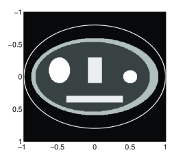
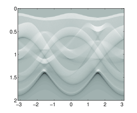
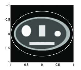
Figure 6.1: Numerical reconstruction using inversion formula (1.9) on the elliptical domain $E=\{\left(x,y\right):x^{2}+\left(y/0.8\right)^{2}<1\}$. Left: Initial data $f$. Middle: Simulated data $\mathcal{U}f$. Right: Numerical reconstruction using inversion formula (1.9).

With $G$ denoting the diverging fundamental solution of the two dimensional wave equation and with $u$ denoting the solution of (1.1), our inversion operator in (1.5) and (1.9) can be written in the form

$$f_{\rm UBP}\left(x_{0}\right)=2\,\nabla_{x_{0}}\cdot\int_{\partial\Omega}\nu_{x}\int_{0}^{\infty}G\left(x-x_{0},t\right)u\left(x,t\right)\mathrm{d}t\mathrm{d}s\left(x\right)\,.$$

The analog of this expression in three spatial dimensions (where $G$ and $u$ are replaced by the three dimensional fundamental solution and the solution of the three dimensional wave equation, respectively) is the so-called universal back-projection introduced in the context of photoacoustic tomography in [27]. In this paper it has also been shown that the universal back-projection formula exactly recovers the initial data of the three dimensional wave equation on spherical domains. This result has been extended to ellipsoids in $\mathbb{R}^{3}$ in [25]. In the latter paper, it is further shown that for any smooth convex bounded domain $\Omega\subset\mathbb{R}^{3}$, the universal back-projection formula recovers the initial data of the three dimensional wave equation modulo the term

$$\left(\mathcal{K}_{\Omega}^{\mathrm{(3D)}}f\right)\left(x_{0}\right)=-\frac{1}{16\pi^{2}}\int_{\Omega}f\left(x_{1}\right)\,\frac{\left(\partial_{a}^{3}\mathcal{R}\chi_{\Omega}\right)\left(\hat{n}\left(x_{1},x_{0}\right),\hat{a}\left(x_{1},x_{0}\right)\right)}{\lvert x_{1}-x_{0}\rvert^{2}}\,\mathrm{d}x_{1}\,.$$

The identities derived in the current paper demonstrate that results similar to the ones of [25] also holds in two spatial dimensions. After initial submission of the present manuscript, these results have actually been generalized to arbitrary dimension (see [32]).

References

• [1] P. Kuchment, L. A. Kunyansky, Mathematics of thermoacoustic and photoacoustic tomography, European J. Appl. Math. 19 (2008) 191–224.
• [2] M. Xu, L. V. Wang, Photoacoustic imaging in biomedicine, Rev. Sci. Instruments 77 (4) (2006) 041101 (22pp).
• [3] P. Burgholzer, J. Bauer-Marschallinger, H. Grün, M. Haltmeier, G. Paltauf, Temporal back-projection algorithms for photoacoustic tomography with integrating line detectors, Inverse Probl. 23 (6) (2007) S65–S80.
• [4] G. Paltauf, R. Nuster, M. Haltmeier, P. Burgholzer, Experimental evaluation of reconstruction algorithms for limited view photoacoustic tomography with line detectors, Inverse Probl. 23 (6) (2007) S81–S94.
• [5] L. E. Andersson, On the determination of a function from spherical averages, SIAM J. Math. Anal. 19 (1) (1988) 214–232.
• [6] S. J. Norton, M. Linzer, Ultrasonic reflectivity imaging in three dimensions: Exact inverse scattering solutions for plane, cylindrical and spherical apertures, IEEE Trans. Biomed. Eng. 28 (2) (1981) 202–220.
• [7] X. L. Dean-Ben, V. Ntziachristos, D. Razansky, Acceleration of optoacoustic model-based reconstruction using angular image discretization, IEEE Trans. Med. Imag. 31 (5) (2012) 1154–1162.
• [8] Y. Dong, T. Görner, S. Kunis, An iterative reconstruction scheme for photoacoustic imaging, Preprint (2011).
• [9] G. Paltauf, J. A. Viator, S. A. Prahl, S. L. Jacques, Iterative reconstruction algorithm for optoacoustic imaging, J. Opt. Soc. Am. 112 (4) (2002) 1536–1544.
• [10] J. Zhang, M. A. Anastasio, X. Pan, L. V. Wang, Weighted expectation maximization reconstruction algorithms for thermoacoustic tomography, IEEE Trans. Med. Imag. 24 (6) (2005) 817–820.
• [11] P. Burgholzer, G. J. Matt, M. Haltmeier, G. Paltauf, Exact and approximate imaging methods for photoacoustic tomography using an arbitrary detection surface, Phys. Rev. E 75 (4) (2007) 046706.
• [12] D. Finch, S. Patch, Rakesh, Determining a function from its mean values over a family of spheres, SIAM J. Math. Anal. 35 (5) (2004) 1213–1240.
• [13] Y. Hristova, P. Kuchment, L. Nguyen, Reconstruction and time reversal in thermoacoustic tomography in acoustically homogeneous and inhomogeneous media, Inverse Probl. 24 (5) (2008) 055006 (25pp).
• [14] P. Stefanov, G. Uhlmann, Thermoacoustic tomography with variable sound speed, Inverse Probl. 25 (7) (2009) 075011 (16pp).
• [15] M. Haltmeier, Frequency domain reconstruction for photo-and thermoacoustic tomography with line detectors, Math. Models Methods Appl. Sci. 19 (2) (2009) 283–306.
• [16] M. Haltmeier, O. Scherzer, P. Burgholzer, R. Nuster, G. Paltauf, Thermoacoustic tomography and the circular Radon transform: exact inversion formula, Math. Models Methods Appl. Sci. 17 (4) (2007) 635–655.
• [17] M. Haltmeier, O. Scherzer, G. Zangerl, A reconstruction algorithm for photoacoustic imaging based on the nonuniform FFT, IEEE Trans. Med. Imag. 28 (11) (2009) 1727–1735.
• [18] K. P. Kostli, D. Frauchiger, J. J. Niederhauser, G. Paltauf, H. P. Weber, M. Frenz, Optoacoustic imaging using a three-dimensional reconstruction algorithm, IEEE Sel. Top. Quant. Electr. 7 (6) (2001) 918–923.
• [19] Y. Xu, M. Xu, L. V. Wang, Exact frequency-domain reconstruction for thermoacoustic tomography–II: Cylindrical geometry, IEEE Trans. Med. Imag. 21 (2002) 829–833.
• [20] J. A. Fawcett, Inversion of $n$-dimensional spherical averages, SIAM J. Appl. Math. 45 (2) (1985) 336–341.
• [21] D. Finch, M. Haltmeier, Rakesh, Inversion of spherical means and the wave equation in even dimensions, SIAM J. Appl. Math. 68 (2) (2007) 392–412.
• [22] M. Haltmeier, A mollification approach for inverting the spherical mean Radon transform, SIAM J. Appl. Math. 71 (5) (2011) 1637–1652.
• [23] L. A. Kunyansky, Explicit inversion formulae for the spherical mean Radon transform, Inverse Probl. 23 (1) (2007) 373–383.
• [24] L. A. Kunyansky, Reconstruction of a function from its spherical (circular) means with the centers lying on the surface of certain polygons and polyhedra, Inverse Probl. 27 (2) (2011) 025012 (22pp).
• [25] F. Natterer, Photo-acoustic inversion in convex domains, Inverse Probl. Imaging 6 (2) (2012) 1–6.
• [26] V. P. Palamodov, A uniform reconstruction formula in integral geometry, Inverse Probl. 28 (6) (2012) 065014.
• [27] M. Xu, L. V. Wang, Universal back-projection algorithm for photoacoustic computed tomography, Phys. Rev. E 71 (1) (2005) 0167061–0167067.
• [28] M. Agranovsky, P. Kuchment, L. Kunyansky, On reconstruction formulas and algorithms for the thermoacoustic tomography, in: L. V. Wang (Ed.), Photoacoustic imaging and spectroscopy, CRC Press, 2009, Ch. 8, pp. 89–101.
• [29] D. Finch, Rakesh, Recovering a function from its spherical mean values in two and three dimensions, in: L. V. Wang (Ed.), Photoacoustic imaging and spectroscopy, CRC Press, 2009, Ch. 7, pp. 77–88.
• [30] F. John, Partial Differential Equations, 4th Edition, Vol. 1 of Applied Mathematical Sciences, Springer Verlag, New York, 1982.
• [31] R. N. Bracewell, The Fourier Transform and its Applications, McGraw Hill, 2000.
• [32] M. Haltmeier, Universal inversion formulas for recovering a function from spherical means, arXiv:1206.3424 [math.AP] (2012).