Fast and Efficient Numerical Methods for an Extended Black-Scholes Model

Abstract

An efficient linear solver plays an important role while solving partial differential equations (PDEs) and partial integro-differential equations (PIDEs) type mathematical models. In most cases, the efficiency depends on the stability and accuracy of the numerical scheme considered. In this article we consider a PIDE that arises in option pricing theory (financial problems) as well as in various scientific modeling and deal with two different topics. In the first part of the article, we study several iterative techniques (preconditioned) for the PIDE model. A wavelet basis and a Fourier sine basis have been used to design various preconditioners to improve the convergence criteria of iterative solvers. We implement a multigrid (MG) iterative method. In fact, we approximate the problem using a finite difference scheme, then implement a few preconditioned Krylov subspace methods as well as a MG method to speed up the computation. Then, in the second part in this study, we analyze the stability and the accuracy of two different one step schemes to approximate the model.

Keywords: convolutional integral; preconditioner; stability; convergence.

1 Introduction

The pricing of options is a central problem in financial investment. It is important in both theoretical and practical point of view since the use of options thrives in the financial market. In option pricing theory, the study of the Black-Scholes equation is very important and interesting (study of a parabolic partial differential equation (PDE)). In recent days, researchers have extended the model by looking at the nonlocal effects, which is a linear partial integro-differential equation (PIDE).

We consider such a partial integro-differential equation [7, 9]

$$\frac{\partial u(x,t)}{\partial t}=\mathcal{L}u(x,t),$$ (1)

where

$$\mathcal{L}u(x,t)=\sigma\frac{\partial^{2}u(x,t)}{\partial x^{2}}+\mu\frac{\partial u(x,t)}{\partial x}-ru(x,t)+\lambda\int_{\Omega}\ J(x-y)\left(u(y,t)-u(x,t)\right)dy,$$

with initial condition

$$u(x,0)=\psi(x),\ -\infty<x<\infty.$$

Here $\sigma\geq 0$, $\lambda\geq 0$, with $(\sigma,\lambda)\neq(0,0)$, $r\geq 0$ and $\mu\in\mathbb{R}$, $J$ is the kernel of the model and $u=u(x,t)$ represents the option price (contingent claim). A normalized kernel function $J(x)$, i.e., $\int_{\Omega}J(x)dx=1$ has been considered in most of the models [10, 12, 17] with suitable parameter values. In general, $J(x-y)$ is a kernel function that models the interaction between options at positions $x$ and $y$. The effect of close neighbours $x$ and $y$ is usually greater than that from more distant ones; this is incorporated in $J$. For simplicity we assume that $J$ is a non-negative function that satisfies smoothness, symmetry and decay conditions. One may consider any $J$ to implement the schemes we discuss in this study. $\frac{1}{2}e^{-|x|}$ and $\sqrt{\frac{\omega}{\pi}}e^{-\omega x^{2}}$ are two sample kernel functions. Boundary conditions are always an issue in these types of models. Here one may easily consider BCs [9]

$$\frac{\partial^{2}u}{\partial x^{2}}=0,\ \text{as }\ x\rightarrow\pm\infty.$$

Operator defined by (1) with $\sigma=0,\mu=0,\ r=0$ comes while modeling phase transitions [10], dynamics of neurons in the brain model [8, 14], and population dynamics models [17] as well.

Numerical approximation and analysis of PDEs and PIDEs using finite difference, finite element method and the pseudo-spectral method are of ongoing research interest. Specially for PIDEs, fast and efficient numerical tools are still to be developed. A clear introduction about option pricing models and some finite difference schemes to approximate the models can be found in [9, 12].

A noble study about the model problem (1) can be found in [12]. The authors consider a European and an American vanilla and barrier options based on the variance gamma process. They discuss derivation of (1) in detail and approximate the model problem numerically by implementing a finite difference algorithm. They present some numerical experiments on the option pricing. But no efficient linear algebra solvers for the discrete equivalent of the model as well as the stability and the accuracy analysis of the approximation are discussed.

In [10], Dugald et. al. consider a nonlocal model of phase transitions of type (1) ($\sigma=0,\ \mu=0,\ r=0$). Stability of stationary solution and coarsening of solutions have been discussed by the authors. They present a finite element scheme to solve the problem and discuss some experimental results.

In [2], the author also considers the nonlocal model of phase transitions. He approximates the problem using the forward Euler scheme and examines the convergence rate of the scheme.

A convolutional model of $\dot{\theta}$ Neuron network has been considered in [3]. The author approximates the problem using finite element method in space, then he applies implicit schemes for time stepping. Then the author analyzes the error in such an approximation.

The PIDE model (1) is well studied in [7]. They discuss viscosity solution of the model followed by a few finite difference approximations. They show that the infinite domain can be truncated to a finite domain $[A,B]$ where $A$ and $B$ depend on the decay of the kernel function $J(x)$. Thus the problem can be considered as a IBVPs. Considering the kernel of the convolution integral as

$$J(x)\equiv J_{\delta}(x)=\sqrt{\frac{1}{2\pi\delta}}\exp\left(-\frac{y^{2}}{2\delta^{2}}\right),$$

the authors in [7] formulate

$$A=+\sqrt{-2\delta^{2}\log(\delta\varepsilon\sqrt{2\pi})},$$

and $B=-A,$ where $\varepsilon>0$ is considered so that $J_{\delta}(x)\geq\varepsilon$. One may consider the model in a spatial periodic domain [2] as well. We use these concepts to approximate the model in a finite as well as a periodic spatial domain.

There are many other articles those discuss these type of models, but to the best of our knowledge the discussion about efficient linear solvers for this type of models is absent. So we focus on some fast and efficient numerical schemes as well as the stability and the accuracy analysis of two finite difference schemes for the operator acting on (1). We start the study by approximating the problem using the backward Euler in time for (1) and investigate some linear algebra tools to speed up the computational process in $\Omega\subset\mathbb{R}$. Then we analyze the stability and the accuracy of two different schemes considering $\Omega=\mathbb{R}$.

The article is organized in the following way. We propose and implement several efficient linear system solvers to compute solutions of (1) in Section 2. Then we discuss the stability of an explicit and an semi-implicit scheme in Section 3. We use Fourier transforms of the integro-differential equation for our analysis throughout this study. The accuracy analysis of two full discrete schemes as well as a semi-discrete approximation are presented in Section 4 and Section 5, respectively. We finish the article with discussion, conclusions and open problems in Section 6.

2 Numerical approximation

Several standard ordinary differential equation solvers are available and can be used to approximate the time derivative. So our main goal, in this study, is to approximate the model (1) in space domain. Here we first perform a time integration, then look for some fast and efficient space integration tools.

Now one may start with the forward Euler scheme for time stepping (an explicit scheme), which uses the values of only previous time step to calculate those of the next. The Algorithm is very simple, in that each unknown, at time step $n+1$, is calculated independently, so it does not require simultaneous solution of equations, and can even be performed easily. But it is unstable for large time steps. We have analyzed the stability condition, and the accuracy of such a scheme in Section 3 and thereafter. Instabilities are big problems in numerical approximation. We want to use large time steps and so we are interested in using implicit schemes.

2.1 An implicit scheme

We start with the implicit Euler scheme for time integration. We approximate the model (1) in time by

$$-\Delta t\sigma\frac{\partial^{2}u^{n}(x)}{\partial x^{2}}-\Delta t\mu\frac{\partial u^{n}(x)}{\partial x}+(1+r\Delta t)u^{n}(x)-\Delta t\lambda\int_{\Omega}\ J(x-y)\left(u^{n}(y)-u^{n}(x)\right)dy=u^{n-1}(x),$$

where $u^{n}(x)=u(x,t_{n})$, $n\geq 0$. We will demonstrate several schemes to approximate the semi-discrete spatial model. For simplicity we write

$$\mathcal{L}u^{n}(x)\equiv\mathcal{L}_{1}(u^{n}(x))+\mathcal{L}_{2}(u^{n}(x))=u^{n-1}(x),$$ (2)

where,

$$\mathcal{L}_{1}(u^{n}(x))=-\Delta t\sigma\frac{\partial^{2}u^{n}(x)}{\partial x^{2}}-\Delta t\mu\frac{\partial u^{n}(x)}{\partial x}+(1+r\Delta t)u^{n}(x),$$

and

$$\mathcal{L}_{2}(u^{n}(x))=-\Delta t\lambda\int_{\Omega}\ J(x-y)\left(u^{n}(y)-u^{n}(x)\right)dy.$$

It is easy to verify that the operator $\mathcal{L}$ acting on (2) is an elliptic partial differential operator [11].

Now it is our aim to design and implement some fast and efficient solvers for (2). We start by approximating

$$\frac{\partial^{2}u^{n}(x)}{\partial x^{2}}=\frac{U^{n}_{i+1}-2U^{n}_{i}+U^{n}_{i-1}}{h^{2}},\quad\frac{\partial u^{n}(x)}{\partial x}=\frac{U^{n}_{i+1}-U^{n}_{i-1}}{2h},$$

and

$$\mathcal{L}_{1}u^{n}(x_{i}) =\sum_{j=-\infty}^{\infty}\int_{\Omega_{i}}J(x_{i}-y)(U^{n}(x_{i})-U^{n}(y))dy$$

$$\approx\sum_{j=-N/2}^{N/2-1}hJ(x_{i}-x_{j})(U^{n}(x_{i})-U^{n}(x_{j})).$$

Based on these approximations we write the full discrete model as

$$AU^{n}=U^{n-1},$$ (3)

which is a system of linear equations with unknown $U^{n}$. The symbol of the discrete equivalent of $\mathcal{L}$ can be written as (see Section 3)

$$A_{syb}(\Delta t,h\xi)=\Delta t\left(1-\tilde{q}(\xi)+\frac{4}{h^{2}}\sin^{2}\left(\frac{h\xi}{2}\right)-\frac{i}{h}\sin(h\xi)\right).$$

Considering

$$g(\Delta t,h\xi)=\frac{1}{A_{syb}(\Delta t,h\xi)}$$

the unknown can be expressed in the Fourier domain as (see Section 3 for details)

$$\tilde{U}^{n}(\xi)=g^{n}(\Delta t,h\xi)\tilde{U}^{0}(\xi).$$

Since,

$$|A_{syb}(\Delta t,h\xi)|\geq 1$$

for any choice of $\Delta t$ and $h$, the scheme is unconditionally stable (a few discrete symbols of this type of operators have been evaluated in detail in next section).

Now the main difficulty of solving linear systems like (3) is that the maximal eigenvalue grows exponentially whereas the minimal eigenvalue is bounded. This situation results in an exponential growth of the condition number

$$cond(A)=\mathcal{O}(N^{2})=\mathcal{O}(2^{2k}),\quad\mbox{ for some $k>1$}.$$

As a result, any iterative solver becomes slower, and a preconditioning is highly needed. To be precise for the Krylov subspace type methods, the solution of the linear system $Au=b$ with some $u_{0}$ is

$$\|u^{j}-u\|_{A}\leq 2\left(\frac{\sqrt{\rho(A)}-1}{\sqrt{\rho(A)}+1}\right)^{j}\|u-u^{0}\|_{A},\ \|x\|_{A}=x^{T}Ax,$$

where $\rho(A)$ is the spectral condition number of $A$. The convergence of the above expression is neat, but it has rarely been presented the convergence of conjugate gradient type methods unless $\rho(A)\approx 1$ [6, page 128]. Thus it becomes clear that one needs to find a matrix $D$ such that

$$B=D^{-1/2}AD^{-1/2}$$

is well conditioned. It is very popular to replace $\rho(A)$ in the iterative solvers by $\rho(B)$, which is called preconditioning [6, 18] and is used for the preconditioned linear system solvers. Thus we get the motivation to develop and to compare a few preconditioned solvers based on the established and popular preconditioning techniques for local second order elliptic operators. We implement and demonstrate the power of multigrid, wavelet as well as Fourier preconditioners. Our goal here is to implement preconditioners in a traditional way so that

1. $D$ is a symmetric and positive definite matrix.

2. $\rho(B)=\mathcal{O}(1)$, as $N\rightarrow\infty$.

To be specific, we discuss several types of preconditioners below.

Wavelet Diagonal Preconditioning:

One of the most successful preconditioners for elliptic PDEs is the wavelet diagonal preconditioning (WDP) which has been studied in details in [18, 22], and many other references. Since $\mathcal{L}$ is of elliptic type we attempt to implement wavelet diagonal preconditioning to solve (3). Suppose $\mathcal{L}$ is defined over a periodic domain. Then a preconditioner can be defined by combining two separate steps:

1. Define a basis transformation $\mathcal{F}$ (wavelet decomposition operator), given by a wavelet transformation, and a wavelet reconstruction operator $\mathcal{F}^{*}$ whose columns are the elements of the wavelet basis denoted by $\psi_{\lambda}$.

2. Define an invertible diagonal scaling matrix $\mathcal{S}$, whose elements are of the form $s_{\lambda}\approx 2^{-2|\lambda|}$, where $|\lambda|$ denotes the scale index of the wavelet.

We consider the symmetric proconditioner

$$D=\mathcal{F}^{*}\mathcal{S}^{1/2}\mathcal{F}$$

as a scaled operator [18, 22]. Then we define the preconditioned operator (equivalent to $\mathcal{L}$ ) by

$$\mathcal{F}^{*}\mathcal{S}^{1/2}\mathcal{F}\mathcal{L}\mathcal{F}^{*}\mathcal{S}^{1/2}\mathcal{F}.$$

A detailed discussion about designing such a preconditioner can be found in [18]. A preconditioner of this type is sensitive with boundary conditions. One may also consider $D=\mathcal{F}^{*}\mathcal{S}\mathcal{F}$ to define a left or a right preconditioner to implement a preconditioned BICG solver. The implementation detail is same as the symmetric preconditioner discussed above.

Fourier Sine Preconditioning:

Localization in the position-wave number space is an important concept in PDEs and can be extended to PIDEs. Most recently, a frame of functions, called windowed Fourier frames, has been employed to solve a variable coefficient second order elliptic PDE [4]. Here it is our aim to design and to implement preconditioners based on the Fourier sine transformation (FSP) for the PIDE (3). This preconditioning is sensitive with boundaries, and works very well for periodic boundary value problems.

The symbol of the operator $\mathcal{L}$ defined by (2) can be written as

$$\Delta t\sigma\xi^{2}-\Delta t\mu i\xi+(1+r\Delta t)-\Delta t\lambda\sqrt{2\pi}(\hat{J}(\xi)-\hat{J}(0)).$$ (4)

When $\xi$ is very large, $\xi^{2}$ term becomes the dominating term in (4) and so $\mathcal{L}$ can be approximated by $\Delta t\sigma\xi^{2}$ in the frequency domain. Thus we approximate

$$\mathcal{L}u\approx\Delta t\sigma\frac{\partial^{2}}{\partial x^{2}}u=\sum\Delta t\sigma\xi_{k}^{2}b_{k}\sin(\xi_{k}x).$$

Let $M_{k}=\Delta t\sigma\xi_{k}^{2}\neq 0$, then

$$\frac{1}{M_{k}}\Delta t\sigma\frac{\partial^{2}}{\partial x^{2}}u\approx\sum_{j\in\mathbb{N}}b_{n}\sin(\xi_{k}x).$$

Thus

$$\left|\frac{1}{M_{k}}\Delta t\sigma\frac{\partial^{2}}{\partial x^{2}}u\right|\approx\left|\sum_{j\in\mathbb{N}}b_{k}\sin(\xi_{k}x)\right|.$$

Now

$$\left|\sum_{j\in\mathbb{N}}b_{k}\sin(\xi_{k}x)\right|^{2} \leq \sum_{j\in\mathbb{N}}|b_{k}|^{2}\leq B\|u\|^{2}$$

where $B$ is the frame upper bound [16]. It is clear from  [16] that $B<\infty$ if we consider a tight frame. Thus

$$\left|\frac{1}{M_{k}}\Delta t\sigma\frac{\partial^{2}}{\partial x^{2}}u\right|<\infty,\quad\text{and so}\quad\left|\frac{1}{M_{k}}\mathcal{L}u\right|<\infty.$$

Based on this idea we define a preconditioned operator

$$P\mathcal{L}P,$$

with the symmetric preconditioner

$$P=F^{*}M^{-1/2}F,$$

where $F$ stands for the Fourier sine transformation operator [16]. The invertibility of the operator $P\mathcal{L}P$, considering $F$ a windowed Fourier transform operator, has been proved in [4] (where $\mathcal{L}$ is a second order elliptic operator). The idea can be extended to the PIDE model that we have considered here. So we avoid attempting to prove the invertibility of the Fourier sine preconditioner (FSP) $P\mathcal{L}P$ here. One may also consider $P=F^{*}M^{-1}F$ to define a left or a right preconditioner to implement a preconditioned BICG solver. The implementation detail is same as the symmetric precomnditioner we have discussed above.

Multigrid Preconditioning:

Multigrid (MG) methods are now a days the fastest and most efficient numerical solvers for linear systems. There are huge recent literatures on MG methods. Actually multigrid method combines two separate ideas [6, 21]:

1. fine grid residual smoothing by relaxation.

2. coarse grid residual correction.

Here the idea is to perform a few iterations (smoothing) in a fine grid, then switch to a coarser level and perform a few iterations, and so on. This is called coarse grid corrections. After corrections, one switches back to the fine grid and performs a few post-smoothing. Thus a multigrid algorithm uses three basic and old steps:

• relaxation step.

• restriction step.

• interpolation step.

A detailed discussion about multigrid can be found in [5, 6, 21] and in many other references. Since the operator (2) is of elliptic type, multigrid would be one of the choices to be considered to verify it’s efficiency. Here we implement a so-called $v-$cycle to solve the system (3). It behaves well with both periodic and non-periodic boundary conditions.

In our problem we use just one $v$-cycle. One can use $\nu$ $v$-cycles if the solution is not sufficiently accurate after the completion of one cycle. We follow the Algorithm 1 for computation.

Algorithm 1.

Multigrid method to solve system of linear equations
To solve the system of linear equations $\mathcal{A}\underline{u}=\underline{f}$ using the multigrid method

INPUT

the finest grid matrix $\mathcal{A}^{h},$ right-hand vector $\underline{f}^{h},$ $L$ the number of steps to travel down the coarsest grid, $\mu$ the number of relaxation(iterations) on each grid, tolerance Tol, number of v-cycles $\nu,$ initial solution $\underline{u}^{h}=\underline{0}$

OUTPUT

The approximate solutions $\underline{u}^{h}.$

Step 1

For $\gamma=1,2,\cdots,\nu$ or error $<$ Tol do the following steps

Step 2

Relax $\mathcal{A}^{h}\underline{u}^{h}=\underline{f}^{h}$ $\mu$ times using the Jacobi iteration with the initial data $\underline{u}_{0}^{h}.$

Step 3

Set $\underline{r}^{h}=\underline{f}^{h}-\mathcal{A}^{h}\underline{u}^{h}.$

Step 4

For $k=2,3,\cdots,L-1$
define residual $\underline{f}^{kh}=\underline{r}^{kh}$, where $r^{kh}_{i}=r^{(k-1)h}_{2i-1}$, $i=1,2,\cdots,\frac{N}{k}$, take the initial guess $\underline{u}_{0}^{kh}=0,$ and relax $\mathcal{A}^{kh}\underline{u}^{kh}=\underline{f}^{kh}$ $\mu$ times as in step 2.

Step 5

Set $\underline{f}^{Lh}=\underline{r}^{Lh}$ and solve $\mathcal{A}^{Nh}\underline{u}^{Lh}=\underline{f}^{Lh}$ exactly.

Step 6

For $k=L-1,L-2,\cdots,1$ we upgrade $\underline{u}^{kh}$ by using

$$u_{2j-1}^{kh} \longleftarrow u_{2j-1}^{kh}+u_{j}^{(k+1)h};\quad j=1,2,\cdots,N_{(k+1)h},$$

$$u_{2j}^{kh} \longleftarrow u_{2j}^{kh}+\frac{1}{2}\left[u_{j}^{(k+1)h}+u_{j+1}^{(k+1)h}\right];\quad j=1,2,\cdots,N_{(k+1)h}-1,$$

$$u_{2N_{(k+1)h}}^{kh} \longleftarrow u_{2N_{(k+1)h}}^{kh}+\frac{1}{2}\left[u_{1}^{(k+1)h}+u_{N_{(k+1)h}}^{(k+1)h}\right]$$

and upgrade the solution $\mu$ times as in step 2.

Step 7

If $\|\underline{u}^{h}\|\leq\mbox{Tol}$ or for $\nu>\gamma>1$ if $\|\underline{u}^{h,\gamma}-\underline{u}^{h,\gamma+1}\|\leq\mbox{Tol},$ output the required solution $\underline{u}^{h}$ else “program stopped after $\nu$ v-cycle”.

STOP

This is to note that one may use FFT for each matrix vector multiplication to reduce the computational costs since the operator $A$ acting on (3) is a toeplitz matrix [13].

2.2 Numerical results and discussions

Here we present some experimental/computer generated results to demonstrate the efficiency of the schemes. We implement the schemes in MATLAB. The MATLAB function ”FFT” is used to define the Fourier sine preconditioner; MATLAB functions ”wavedec”, and ”waverec” have been used for the wavelet diagonal preconditioner with the Daubechies wavelet ’db6’. Here we consider a spatial periodic $[0\ 1]$ domain and

$$J(x)=\sum_{r=-\infty}^{\infty}J^{\infty}(x-r)\quad\text{with}\quad J^{\infty}(x)=\sqrt{\frac{100}{\pi}}e^{-100x^{2}}.$$

A detailed discussion about such a consideration of the kernel function can be found in [3]. We consider $\sigma=0.01$, $\mu=0.01$, $r=0.01$, $\lambda=0.1$, $\delta=100$ for all the numerical results presented here.

In Figure 1, we present condition numbers of the preconditioned operators $P\mathcal{L}P$, and $D\mathcal{L}D$, as well as the condition number of $\mathcal{L}$. We notice that $\rho(D\mathcal{L}D)$, and $\rho(P\mathcal{L}P)$ are of $\mathcal{O}(1)$, where as $\rho(\mathcal{L})$ is of $\mathcal{O}(N^{2})$. Then, in Figure 2, we compare the number of iterations taken by the preconditioned solvers for a set of $N$ values. We notice that the preconditioned systems converge in a few iterations and the number of iterations is independent of the system size.

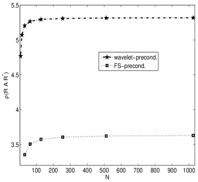
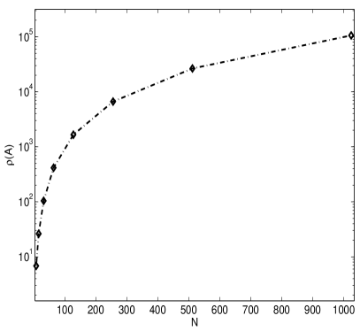
Figure 1: Left Figure: Condition numbers of the wavelet preconditioned operator, and the Fourier sine preconditioned operator, both are of $\mathcal{O}(1)$, Right Figure: Condition number of $A$, which is of $\mathcal{O}(N^{2})$.

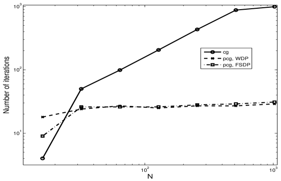
Figure 2: The Number of iterations taken to converge by the conjugate gradient, the WDP conjugate gradient and the FSP conjugate gradient methods to solve (3) considering $\Delta t=0.01$.

Then we demonstrate the total CPU time taken to solve the linear system by the solvers MG, WDP CG and FSP CG respectively to see the time efficiency of the techniques in Figure 3. Here we observe that in terms of CPU time the MG out performs all other schemes. In fact, the MG method takes very little computational time compared to the other two. The WDP and FSP techniques take most of the time to define the preconditioners, the preprocessing steps to use preconditioned linear system solvers.

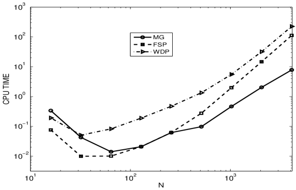
Figure 3: CPU time taken to converge by the WDP, the FSP and the MG methods for various choices of system size. For the multigrid method we consider one $\log 2(N)-2$ level $v-$cycle with one SOR iteration with $\omega=1.2$ in all levels but the coarsest one. In the coarsest level we solve the system exactly. We use Intel(R) Core(TM) i3 CPU M380 at 2.53 GHz processor with ram 2.00 GB. Here we solve (3) considering $\Delta t=0.01$, and by varying spatial grid points $N$, and $u_{0}(x)=\exp[-100(x-.5)^{2}]$.

2.3 An explicit implicit scheme

While solving the linear system (3) we notice that $A$ is a full matrix. Thus matrix vector multiplications are computationally costly. To reduce the computation cost further we look for an another scheme that may reduce computational costs. We implement an explicit implicit scheme where $A$ becomes a spare matrix, thus reduces computation costs in matrix vector multiplications.

We approximate the model (1) in time by

$$-\Delta t\sigma\frac{\partial^{2}u^{n}(x)}{\partial x^{2}}+(1+r\Delta t)u^{n}(x)=u^{n-1}(x)+\Delta t\mu\frac{\partial u^{n-1}(x)}{\partial x}+\Delta t\lambda\int_{\Omega}\ J(x-y)\left(u^{n-1}(y)-u^{n-1}(x)\right)dy,$$

where $u^{n}(x)=u(x,t_{n})$, $n\geq 0$. For simplicity we write

$$\mathcal{L}_{1}(u^{n}(x))=\mathcal{L}_{2}u^{n-1}(x),$$ (5)

where

$$\mathcal{L}_{1}(u^{n}(x))=-\Delta t\sigma\frac{\partial^{2}u^{n}(x)}{\partial x^{2}}+(1+r\Delta t)u^{n}(x),$$

and

$$\mathcal{L}_{2}(u^{n}(x))=\Delta t\mu\frac{\partial u^{n-1}(x)}{\partial x}+\Delta t\lambda\int_{\Omega}\ J(x-y)\left(u^{n-1}(y)-u^{n-1}(x)\right)dy.$$

The operator $\mathcal{L}_{1}$ is an elliptic partial differential operator [11]. After the time integration, the right hand side of (5) is a known vector and explicitly depends on $u^{n-1}$, $n\geq 1$. Thus all the linear algebra tools we discussed above for (2) are applicable to (5), and they are indeed, efficient schemes for elliptic PDEs.

To justify our claim we implement the MG method, the fastest tool we implemented in the previous section, to solve the linear system obtained from (5). We compare the CPU time taken to solve the linear system obtained by the implicit solver and the explicit implicit solver (5) in Figure 4. Here we notice that the scheme (2) and the explicit implicit scheme (5) are comparable. In fact, it is observed from Figure 4 that the scheme (5) requires a minimum CPU time to converge compared to all other solvers.

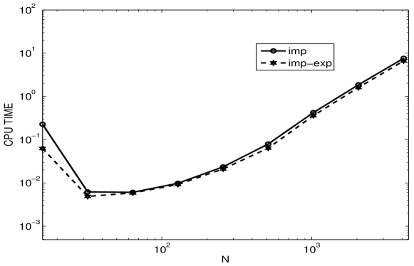
Figure 4: CPU time taken to converge by MG methods for various choices of system size from the implicit as well as the explicit implicit solvers. Here we consider one $\log 2(N)-2$ level $v-$cycle with one SOR iteration with $\omega=1.2$ in all levels but the coarsest one. In the coarsest level we solve the system exactly. We use Intel(R) Core(TM) i3 CPU M380 at 2.53 GHz processor with ram 2.00 GB. Here we solve (3) and (5) considering $\Delta t=0.01$, and by varying spatial grid points $N$, and $u_{0}(x)=\exp[-100(x-.5)^{2}]$.

3 Stability analysis

From the above Section we see that the scheme (5) dominates the implicit scheme in terms of computational time. This numerical experiment motivates us to analyze the stability and the accuracy of an explicit and an explicit implicit scheme. For the simplicity of the stability analysis we consider $\sigma=\mu=\lambda=r=1$. Here we analyze the stability of the forward Euler scheme (explicit) and a mix Euler scheme (explicit implicit). We consider the linear partial integro-differential equation [9] (an IVP)

$$u_{t}(x,t)=-u+u_{x}+u_{xx}+\int_{-\infty}^{\infty}J(x-y)\left(u(y,t)-u(x,t)\right)dy$$ (6)

with $u(x,t_{0})=u_{0}(x),$ $x\in\mathbb{R}.$ This IVP can be approximated in space by

$$\frac{dU_{j}(t)}{dt} = \frac{U_{j+1}-2U_{j}+U_{j-1}}{h^{2}}+\frac{U_{j+1}-U_{j-1}}{2h}-U_{j}$$ (7)

$$\qquad+\qquad h\sum_{k=-\infty}^{\infty}J(x_{j}-x_{k})(U_{k}-U_{j})$$

for each $j\in\mathbb{Z}$ where $U_{j}(t)\approx u(x_{j},t)$ and $x_{j}=jh$ where $h$ is the uniform spacing between the grid points $x_{j}$ and $x_{j+1}$ for all $j\in\mathbb{Z}$. We need the following definitions to support our study.

For the sequence $\{v_{m}:m\in\mathbb{Z}\}$ on the mesh points $\{x_{m}=mh:m\in\mathbb{Z}\}$ the discrete Fourier Transform (DFT) is defined by

$$\tilde{v}(\xi)=\frac{h}{\sqrt{2\pi}}\sum_{m=-\infty}^{\infty}e^{-ihm\xi}v_{m}$$ (8)

if $v_{m}\in L_{2}(h\mathbb{Z})$, and its inverse is

$$v_{m}=\frac{1}{\sqrt{2\pi}}\int_{-\frac{\pi}{h}}^{\frac{\pi}{h}}e^{ihm\xi}\tilde{v}(\xi)d\xi$$ (9)

where $\xi\in[\frac{-\pi}{h},\frac{\pi}{h}].$ Parseval’s Formulae  [19, 23] are defined as

$$||\tilde{v}||_{h}^{2}=\int_{-\frac{\pi}{h}}^{\frac{\pi}{h}}|\tilde{v}(\xi)|^{2}d\xi=\sum_{m=-\infty}^{\infty}h|v_{m}|^{2}=||v||_{h}^{2}.$$ (10)

An explicit scheme

We apply the explicit Euler scheme to the semi-discrete model (7) to obtain

$$U_{j}^{n+1}-U_{j}^{n} = -\Delta tU_{j}^{n}+\Delta t\frac{U_{j+1}^{n}-U_{j-1}^{n}}{2h}+\Delta t\frac{U_{j+1}^{n}-2U_{j}^{n}+U_{j-1}^{n}}{h^{2}}$$

$$\qquad+\qquad h\Delta t\sum_{k=-\infty}^{\infty}J(x_{j}-x_{k})\left(U_{k}^{n}-U_{j}^{n}\right)$$

where $U_{j}^{n}=U(x_{j},t_{n}).$ This is equivalent to

$$U_{j}^{n+1} = \Delta t\frac{U_{j+1}^{n}-U_{j-1}^{n}}{2h}+\Delta t\frac{U_{j+1}^{n}-2U_{j}^{n}+U_{j-1}^{n}}{h^{2}}+U_{j}^{n}\left(1-\Delta t-h\Delta t\sum_{k=-\infty}^{\infty}J(x_{j}-x_{k})\right)$$ (11)

$$\qquad+h\Delta t\sum_{k=-\infty}^{\infty}J(x_{j}-x_{k})U_{k}^{n}.$$

We multiply (11) by $\frac{h}{\sqrt{2\pi}}e^{-ijh\xi}$ and sum over all $j$ to obtain

$$\frac{h}{\sqrt{2\pi}}\sum_{j=-\infty}^{\infty}e^{-ijh\xi}U_{j}^{n+1} = \frac{h}{\sqrt{2\pi}}\sum_{j=-\infty}^{\infty}e^{-ijh\xi}U_{j}^{n}\left(1-\Delta t-h\Delta t\sum_{k=-\infty}^{\infty}J(x_{j}-x_{k})\right)$$

$$+\frac{h}{\sqrt{2\pi}}\sum_{k=-\infty}^{\infty}e^{-ikh\xi}U_{k}^{n}\left[h\Delta t\sum_{j=-\infty}^{\infty}J(x_{j}-x_{k})e^{-i(j-k)h\xi}\right]$$

$$+\frac{h}{\sqrt{2\pi}}\sum_{j=-\infty}^{\infty}e^{-ijh\xi}\left(\Delta t\frac{U_{j+1}^{n}-2U_{j}^{n}+U_{j-1}^{n}}{h^{2}}\right)$$

$$+\frac{h}{\sqrt{2\pi}}\sum_{j=-\infty}^{\infty}e^{-ijh\xi}\left(\Delta t\frac{U_{j+1}^{n}-U_{j-1}^{n}}{2h}\right).$$

So using $J(x)=J(-x)$ we have

$$\tilde{U}^{n+1}(\xi) = \left\{1-\Delta t+h\Delta t\sum_{j=-\infty}^{\infty}J(x_{j}-x_{k})\left(e^{i(k-j)h\xi}-1\right)\right\}\tilde{U}^{n}(\xi)$$

$$+\frac{\Delta t}{h^{2}}\tilde{U}^{n}(\xi)\left(e^{ih\xi}+e^{-ih\xi}-2\right)+\frac{\Delta t}{2h}\tilde{U}^{n}(\xi)\left(e^{ih\xi}-e^{-ih\xi}\right).$$

Thus

$$\tilde{U}^{n}(\xi)=\left(g(h\xi,\Delta t)\right)^{n}\tilde{U}^{0}(\xi),$$ (12)

where

$$g(h\xi,\Delta t) = 1-\Delta t+\Delta t\left(h\sum_{r=-\infty}^{\infty}e^{-irh\xi}J(x_{r})-h\sum_{r=-\infty}^{\infty}e^{-irh0}J(x_{r})\right)$$ (13)

$$+\frac{\Delta t}{h^{2}}\left(e^{ih\xi}+e^{-ih\xi}-2\right)+\frac{\Delta t}{2h}\left(e^{ih\xi}-e^{-ih\xi}\right)$$

$$= 1-\Delta t+\sqrt{2\pi}\Delta t\left(\tilde{J}(\xi)-\tilde{J}(0)\right)-4\frac{\Delta t}{h^{2}}\sin^{2}{\frac{h\xi}{2}}+\frac{i\Delta t}{h}\sin(h\xi).$$

Now we carry out the stability analysis of (11) following [1, 19]. We need the following Lemma to bound $g(h\xi,\Delta t).$

Proposition 1.

Assume that $J(x)\in L_{2}(\mathbb{R})\cap C(\mathbb{R})$ satisfies

H1

$J(x)\geq 0;$

H2

$J(x)$ is normalized such that $\int_{-\infty}^{\infty}J(x)dx=1;$

H3

$J(x)$ is symmetric, i.e. $J(x)=J(-x),$ for all $x\in\mathbb{R};$

H4

$J(x)$ is decreasing on $(0,\infty);$

H5

$\hat{J}(\xi)\geq 0.$

Then H1 - H4 give the DFT results $0\leq\tilde{J}(0)$ and $\tilde{J}(\xi)\leq\tilde{J}(0)\leq\sqrt{\frac{2}{\pi}}+\tilde{J}(\xi)$ for all $\xi\in[-\frac{\pi}{h},\frac{\pi}{h}]$ and the CFT results $\hat{J}(\xi)\leq\hat{J}(0)\leq\sqrt{\frac{2}{\pi}}+\hat{J}(\xi).$ Further, if $\mathbf{H5}$ holds, then $\tilde{J}(\xi)\geq 0$ for all $J\in H^{r}(\mathbb{R})$, $r>\frac{1}{2}$, [2].

Now we back to the main discussion. The scheme is stable if

$$|g|\leq 1.$$

Here

$$|g|^{2} = \left(1-\Delta t+\sqrt{2\pi}\Delta t(\tilde{J}(\xi)-\tilde{J}(0))-\frac{4\Delta t}{h^{2}}\sin^{2}\left(\frac{h\xi}{2}\right)\right)^{2}$$

$$\qquad+\qquad\left(\frac{\Delta t}{h}\right)^{2}\sin^{2}\left(h\xi\right)\leq 1$$

gives

$$\Delta t\left(1+\tilde{q}^{2}(\xi)-2\tilde{q}(\xi)+\frac{8}{h^{2}}\sin^{2}\left(\frac{h\xi}{2}\right)-\frac{8\tilde{q}(\xi)}{h^{2}}\sin^{2}\left(\frac{h\xi}{2}\right)+\right.$$

$$\left.\frac{16}{h^{4}}\sin^{4}\left(\frac{h\xi}{2}\right)+\frac{1}{h^{2}}\sin^{2}h\xi\right)\leq\left(2-2\tilde{q}(\xi)+\frac{8}{h^{2}}\sin^{2}\frac{h\xi}{2}\right).$$

Thus applying Proposition 1 we have

$$\Delta t\left(9+\frac{25}{h^{2}}+\frac{16}{h^{4}}\right)\leq 4,$$

and so

$$\Delta t\leq\frac{4h^{4}}{(3h^{2}+4)^{2}+h^{2}}\leq\frac{4h^{4}}{(3h^{2}+4)^{2}}=\frac{4}{(3+4/h^{2})^{2}}.$$ (14)

Theorem 1.

If $J(x)$ is a normalized symmetric nonnegative function and $J\in L_{2}(\mathbb{R})\cap C(\mathbb{R})$ then there exists $0<\frac{4}{(3+4/h^{2})^{2}}\leq\Delta t^{*}$ such that

$$\|U^{n}\|_{h}\leq\|U^{0}\|_{h}$$

for all $0<\Delta t\leq\Delta t^{*}$ and $n\geq 0.$

Proof.

The proof easily follows from perseval’s relation. ∎

Thus in the discrete $L_{2}$ norm, (11) is a stable scheme [19, Definition 1.5.1] with the stability condition (14).

An explicit implicit scheme

Applying a mixed Euler scheme we write a full discrete version of the model (6) by

$$U_{j}^{n+1}-U_{j}^{n} = -\Delta tU_{j}^{n+1}+\Delta t\frac{U_{j+1}^{n}-U_{j}^{n}}{h}+\Delta t\frac{U_{j+1}^{n+1}-2U_{j}^{n+1}+U_{j-1}^{n+1}}{h^{2}}$$

$$\qquad+\qquad h\Delta t\sum_{k=-\infty}^{\infty}J(x_{j}-x_{k})\left(U_{k}^{n}-U_{j}^{n}\right)$$

where $U_{j}^{n}=U(x_{j},t_{n}).$ This is equivalent to

$$U_{j}^{n+1}\left(1+\Delta t\right) = \Delta t\frac{U_{j+1}^{n}-U_{j}^{n}}{2h}+\Delta t\frac{U_{j+1}^{n+1}-2U_{j}^{n+1}+U_{j-1}^{n+1}}{h^{2}}+U_{j}^{n}\left(1-h\Delta t\sum_{k=-\infty}^{\infty}J(x_{j}-x_{k})\right)$$ (15)

$$\qquad+h\Delta t\sum_{k=-\infty}^{\infty}J(x_{j}-x_{k})U_{k}^{n}.$$

Multiplying (15) by $\frac{h}{\sqrt{2\pi}}e^{-ijh\xi}$ and summing over all $j$ we get

$$(1+\Delta t)\frac{h}{\sqrt{2\pi}}\sum_{j=-\infty}^{\infty}e^{-ijh\xi}U_{j}^{n+1} = \frac{h}{\sqrt{2\pi}}\sum_{j=-\infty}^{\infty}e^{-ijh\xi}U_{j}^{n}\left(1-h\Delta t\sum_{k=-\infty}^{\infty}J(x_{j}-x_{k})\right)$$

$$+\frac{h}{\sqrt{2\pi}}\sum_{k=-\infty}^{\infty}e^{-ikh\xi}U_{k}^{n}\left[h\Delta t\sum_{j=-\infty}^{\infty}J(x_{j}-x_{k})e^{-i(j-k)h\xi}\right]$$

$$+\frac{h}{\sqrt{2\pi}}\sum_{j=-\infty}^{\infty}e^{-ijh\xi}\left(\Delta t\frac{U_{j+1}^{n+1}-2U_{j}^{n+1}+U_{j-1}^{n+1}}{h^{2}}\right)$$

$$+\frac{h}{\sqrt{2\pi}}\sum_{j=-\infty}^{\infty}e^{-ijh\xi}\left(\Delta t\frac{U_{j+1}^{n}-U_{j}^{n}}{h}\right).$$

So using $J(x)=J(-x)$

$$\tilde{U}^{n+1}(\xi)(1+\Delta t-\frac{\Delta t}{h^{2}}\left(e^{ih\xi}+e^{-ih\xi}-2\right)) = \left\{1+h\Delta t\sum_{j=-\infty}^{\infty}J(x_{j}-x_{k})\left(e^{i(k-j)h\xi}-1\right)\right\}\tilde{U}^{n}(\xi)$$

$$+\frac{\Delta t}{2h}\tilde{U}^{n}(\xi)\left(e^{ih\xi}-1\right)$$

giving

$$\tilde{U}^{n+1}(\xi)=g(h\xi,\Delta t)\tilde{U}^{n}(\xi).$$

And we write

$$\tilde{U}^{n}(\xi)=\left(g(h\xi,\Delta t)\right)^{n}\tilde{U}^{0}(\xi),$$ (16)

where

$$g(h\xi,\Delta t) = \frac{1+\sqrt{2\pi}\Delta t\left(\tilde{J}(\xi)-\tilde{J}(0)\right)+\frac{\Delta t}{h}\left(e^{ih\xi}-1\right)}{1+\Delta t+4\frac{\Delta t}{h^{2}}\sin^{2}{\frac{h\xi}{2}}}.$$ (17)

The scheme is stable if

$$\left|1+\sqrt{2\pi}\Delta t\left(\tilde{J}(\xi)-\tilde{J}(0)\right)+\frac{\Delta t}{h}\left(e^{ih\xi}-1\right)\right|\leq\left|1+\Delta t+4\frac{\Delta t}{h^{2}}\sin^{2}{\frac{h\xi}{2}}\right|$$

which gives

$$\left(1+\sqrt{2\pi}\Delta t\left(\tilde{J}(\xi)-\tilde{J}(0)\right)-\frac{\Delta t}{h}\right)^{2}+\left(\frac{\Delta t}{h}\right)^{2}\leq\left(1+\Delta t+4\frac{\Delta t}{h^{2}}\sin^{2}{\frac{h\xi}{2}}\right)^{2}.$$

Now

$$\left(1+\Delta t\right)^{2}\leq\left(1+\Delta t+4\frac{\Delta t}{h^{2}}\sin^{2}{\frac{h\xi}{2}}\right)^{2},$$

and

$$0\leq\left|\sqrt{2\pi}\left(\tilde{J}(\xi)-\tilde{J}(0)\right)\right|\leq 2.$$

Simplifying the above inequality we get

$$\Delta t^{2}\left(\tilde{q}^{2}(\xi)-1+\frac{2}{h^{2}}-\frac{2}{h}\tilde{q}(\xi)\right)\leq\Delta t\left(2+\frac{2}{h}-2\tilde{q}(\xi)\right),$$

and so

$$\Delta t\leq\frac{2h(h+1)}{3h^{2}+4h+2}.$$ (18)

Theorem 2.

If $J(x)$ is a normalized symmetric nonnegative function and $J\in L_{2}(\mathbb{R})\cap C(\mathbb{R})$ then there exists $0<\frac{2h(h+1)}{3h^{2}+4h+2}\leq\Delta t^{*}$ such that

$$\|U^{n}\|_{h}\leq\|U^{0}\|_{h}$$

for all $0<\Delta t\leq\Delta t^{*}$ and $n\geq 0.$

Proof.

The proof easily follows from perseval’s relation. ∎

Thus in the discrete $L_{2}$ norm, (15) is a stable scheme [19, Definition 1.5.1] with the stability condition (18). We demonstrate maximum values of $\Delta t$ from both (14) and (18) respectively in Figure 5 for various choices of $h$. It shows the dominance of the semi-implicit scheme.

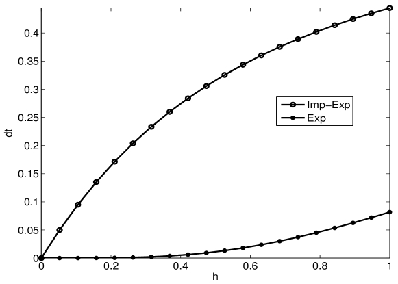
Figure 5: Maximum choices of $\Delta t$ from the inequalities (14) and (18).

Computational algorithm

From the schemes (12) and (16) it follows that the DFT gives a each way to compute numerical solutions. The approximate solution $U^{n}(\cdot)$ can be computed in the spatial domain simply, accurately and rapidly using the following steps. For faster computations, one may precompute the FFT of $u_{0}$, $J(x)$, and $J(0)$.

1. Compute the fast Fourier transform (FFT) of $u_{0}$.

2. Compute $g$ using the FFT of $J$.

3. Evaluate $g^{n}$ and multiply with the result in step $1$.

4. Compute the inverse FFT of the product defined in step $3$.

4 Accuracy analysis

Applying the continuous Fourier transform (6) can be written as

$$\hat{u}_{t}(\xi,t)=\hat{q}(\xi)\hat{u}(\xi,t),$$ (19)

where

$$\hat{q}(\xi)=\sqrt{2\pi}\left(\frac{-1}{\sqrt{2\pi}}+\hat{J}(\xi)-\hat{J}(0)-\frac{\xi^{2}}{\sqrt{2\pi}}+\frac{i\xi}{\sqrt{2\pi}}\right).$$

Thus the exact solution of (19) in the frequency domain is

$$\hat{u}(\xi,t)=e^{\hat{q}(\xi)t}\hat{u}_{0}(\xi).$$ (20)

Here it is easy to verify that $\Re(\hat{q})\leq 0$ (Proposition 1, which is presented in Section 3) which gives the stability property $|\hat{u}(\xi,t)|\leq|\hat{u}_{0}(\xi,t)|.$

Computational algorithm

The following steps can be taken to compute the exact solution and the error in schemes (12) and (16).

1. Compute the FFT of $u_{0}$.

2. Compute $\hat{q}$ as defined in (19) using FFT of $\hat{J}$.

3. Evaluate $\exp(n\Delta t\hat{q})$ and multiply with the result obtained from step $1$.

4. Compute the inverse FFT of the product defined in $3$.

5. Evaluate $\|u(\cdot,t)-U^{n}(\cdot)\|$.

In this section it is our aim to present a theoretical bound of the error term $\|u-U^{n}\|$. Now we carry out the convergence analysis of (11) and (15) following [19]. We apply the inverse CFT on (20) to get

$$u(x,t)=\frac{1}{\sqrt{2\pi}}\int_{-\infty}^{\infty}e^{ix\xi}e^{\hat{q}(\xi)t}\hat{u}_{0}(\xi)d\xi,$$ (21)

which is the exact solution of (6).

4.1 The explicit scheme (12)

Using the inverse DFT formula (9) on (12), the approximate solution can be presented as

$$U_{m}^{n}=\frac{1}{\sqrt{2\pi}}\int_{-\frac{\pi}{h}}^{\frac{\pi}{h}}e^{imh\xi}\left(g(h\xi,\Delta t)\right)^{n}\tilde{u}_{0}(\xi)d\xi.$$ (22)

Applying the Fourier interpolation [19] the mesh function (22) can be written as

$$\mathcal{S}U^{n}(x)=\frac{1}{\sqrt{2\pi}}\int_{-\frac{\pi}{h}}^{\frac{\pi}{h}}e^{ix\xi}\left(g(h\xi,\Delta t)\right)^{n}\tilde{u}_{0}(\xi)d\xi.$$ (23)

Thus

$$u(x,t_{n})-\mathcal{S}U^{n}(x)=\frac{1}{\sqrt{2\pi}}\int_{|\xi|\leq\frac{\pi}{h}}e^{ix\xi}\left(e^{\hat{q}(\xi)t_{n}}\hat{u}_{0}(\xi)-\left(g(h\xi,\Delta t)\right)^{n}\tilde{u}_{0}(\xi)\right)d\xi$$

$$+\frac{1}{\sqrt{2\pi}}\int_{|\xi|>\frac{\pi}{h}}e^{ix\xi}e^{\hat{q}(\xi)t_{n}}\hat{u}_{0}(\xi)d\xi.$$ (24)

So

$$\|u(x,t_{n})-\mathcal{S}U^{n}(x)\|^{2} \leq \frac{1}{\sqrt{2\pi}}\int_{|\xi|\leq\frac{\pi}{h}}\left|e^{\hat{q}(\xi)t_{n}}\hat{u}_{0}(\xi)-\left(g(h\xi,\Delta t)\right)^{n}\tilde{u}_{0}(\xi)\right|^{2}d\xi$$ (25)

$$+\frac{1}{\sqrt{2\pi}}\int_{|\xi|>\frac{\pi}{h}}\left|\hat{u}_{0}(\xi)\right|^{2}d\xi,$$

using Parseval’s relation and the stability property $\hat{q}\leq 0$.

Let us find a bound related to the-evolution error first. Here

$$\frac{1}{\sqrt{2\pi}}\int_{|\xi|\leq\frac{\pi}{h}}\left|e^{\hat{q}(\xi)t_{n}}\hat{u}_{0}(\xi)-g(h\xi,\Delta t)^{n}\tilde{u}_{0}(\xi)\right|^{2}d\xi$$

$$\leq \sqrt{\frac{2}{\pi}}\int_{|\xi|\leq\frac{\pi}{h}}\left|e^{\hat{q}(\xi)t_{n}}-g(h\xi,\Delta t)^{n}\right|^{2}|\hat{u}_{0}(\xi)|^{2}d\xi+\sqrt{\frac{2}{\pi}}\int_{|\xi|\leq\frac{\pi}{h}}\left|\sum_{j\neq 0}\hat{u}_{0}\left(\xi+\frac{2\pi j}{h}\right)\right|^{2}d\xi,$$

since $\left|g(h\xi,\Delta t)\right|\leq 1.$ Now following [19, page 204], [2]

$$\sqrt{\frac{2}{\pi}}\int_{|\xi|\leq\frac{\pi}{h}}\left|\sum_{j\neq 0}\hat{u}_{0}\left(\xi+\frac{2\pi j}{h}\right)\right|^{2}d\xi \leq C_{1}(\sigma)h^{2\sigma}\|u_{0}\|_{H^{\sigma}(\mathbb{R})}^{2},$$ (26)

where $C_{1}(\sigma)=2\left(\frac{1}{\pi}\right)^{2\sigma}\sum_{j=1}^{\infty}\left(2j-1\right)^{-2\sigma}$ assuming that the initial function is smooth and there exists $\sigma>\frac{1}{2}$ such that $\|u_{0}\|_{H^{\sigma}(\mathbb{R})}$ is bounded, and

$$\frac{1}{\sqrt{2\pi}}\int_{|\xi|>\frac{\pi}{h}}|\hat{u}_{0}(\xi)|^{2}d\xi \leq C_{2}(\sigma)h^{2\sigma}\|u_{0}\|_{H^{\sigma}(\mathbb{R})}^{2}.$$ (27)

When $t_{n}=n\Delta t$

$$e^{\hat{q}(\xi)t_{n}}-g(h\xi,\Delta t)^{n}={e^{\hat{q}(\xi)\Delta t}}^{n}-g^{n}=(e^{\hat{q}(\xi)\Delta t}-g)\sum_{r=0}^{n-1}{e^{\hat{q}(\xi)\Delta t}}^{n-r}g^{r}.$$

Since $\hat{q}(\xi)\leq 0$ and $|g(h\xi,\Delta t)|\leq 1$ we have

$$|{e^{\hat{q}(\xi)\Delta t}}^{n}-g^{n}|\leq n|e^{\hat{q}(\xi)\Delta t}-g|,$$

or equivalently

$$\left|e^{\hat{q}(\xi)t_{n}}-{g(h\xi,\Delta t)}^{n}\right|\leq n|e^{\hat{q}(\xi)\Delta t}-g(h\xi,\Delta t)|.$$ (28)

Now, for the scheme (11),

$$e^{\Delta t\hat{q}(\xi)}-g(h\xi,\Delta t) = e^{\Delta t\sqrt{2\pi}\left(\hat{J}(\xi)-\hat{J}(0)-\frac{\xi^{2}+1}{\sqrt{2\pi}}+\frac{i\xi}{\sqrt{2\pi}}\right)}-\left(1-\Delta t+\Delta t\sqrt{2\pi}\left(\tilde{J}(\xi)-\tilde{J}(0)\right)\right.$$ (29)

$$\left.-4\frac{\Delta t}{h^{2}}\sin^{2}\frac{h\xi}{2}+\frac{i\Delta t}{h}sin(h\xi)\right)$$

$$= \Delta t\sqrt{2\pi}\left(\hat{J}(\xi)-\hat{J}(0)-\frac{\xi^{2}+1}{\sqrt{2\pi}}+\frac{i\xi}{\sqrt{2\pi}}\right)-\Delta t\sqrt{2\pi}\left(\tilde{J}(\xi)-\tilde{J}(0)\right.$$

$$\left.-\frac{4}{\sqrt{2\pi}h^{2}}\sin^{2}\frac{h\xi}{2}+\frac{i\Delta t}{h}sin(h\xi)-1\right)$$

$$+\sum_{j=2}^{\infty}\frac{\Delta t^{j}}{j!}\left(\sqrt{2\pi}\left(\hat{J}(\xi)-\hat{J}(0)-\frac{\xi^{2}+1}{\sqrt{2\pi}}+\frac{i\xi}{\sqrt{2\pi}}\right)\right)^{j}.$$

Assuming that $J\in H^{r}(\mathbb{R})$ with $r>\frac{1}{2}$ and applying the Poisson summation formula, (29) becomes

$$e^{\Delta t\hat{q}(\xi)}-g(h\xi,\Delta t) = -\Delta t\sqrt{2\pi}\sum_{j\neq 0}\left(\hat{J}(\xi+\frac{2\pi j}{h})-\hat{J}(\frac{2\pi j}{h})\right)+\frac{4\Delta t}{h^{2}}\sin^{2}\left(\frac{h\xi}{2}\right)-\Delta t\xi^{2}$$ (30)

$$\qquad+i\Delta t\xi-\frac{i\Delta t}{h}\sin\left(h\xi\right)+\mathcal{O}(\Delta t^{2})$$

$$= -\Delta t\sqrt{2\pi}\sum_{j\neq 0}\left(\hat{J}(\xi+\frac{2\pi j}{h})-\hat{J}(\frac{2\pi j}{h})\right)+\mathcal{O}\left(\left(\frac{h\xi}{2}\right)^{4}\right)$$

$$+\frac{i\Delta t}{h}\left(h\xi\right)^{3}+\mathcal{O}((h\xi)^{5})+\mathcal{O}(\Delta t^{2}).$$

Proposition 2.

[2] Assume that H1, H3 and H5 of Lemma 1 hold and in addition, the following condition holds:

H6.

$\frac{d}{d\xi}\hat{J}(\xi)\leq 0$ for $\xi\geq 0.$

Then, for all $|\xi|\leq\frac{\pi}{h},$ $\qquad\left|\sum_{j\neq 0}\left(\hat{J}(\xi+\frac{2\pi j}{h})-\hat{J}(\frac{2\pi j}{h})\right)\right|\leq 2\hat{J}(\frac{\pi}{h}).$

Thus applying Proposition 2, (30) can be written as

$$|e^{\Delta t\hat{q}(\xi)}-g(h\xi,\Delta t)| \leq \Delta tC_{1}(h)+C_{2}\Delta th^{2}|\xi|^{4}$$ (31)

where $C_{1}(h)=2\sqrt{2\pi}\hat{J}(\frac{\pi}{h}).$ If $J\in L_{2}(\mathbb{R})$, then $|\hat{J}(\xi)|\rightarrow 0$ as $|\xi|\rightarrow\infty$  [15], [20, page 30]. The rate of convergence determines the accuracy of the scheme. We have

$$\int_{|\xi|\leq\frac{\pi}{h}}\left|\left(e^{\hat{q}(\xi)t_{n}}-g(h\xi,\Delta t)^{n}\right)\hat{u}_{0}(\xi)\right|^{2}d\xi$$ (32)

$$\leq \int_{|\xi|\leq\frac{\pi}{h}}n^{2}\left|e^{\hat{q}(\xi)\Delta t}-g(h\xi,\Delta t)\right|^{2}|\hat{u}_{0}(\xi)|^{2}d\xi,\quad\mbox{using (\ref{vnaa11:f})}$$

$$\leq n^{2}\int_{|\xi|\leq\frac{\pi}{h}}\left|\Delta tC_{1}(h)+C_{2}\Delta th^{2}|\xi|^{3}\right|^{2}|\hat{u}_{0}(\xi)|^{2}d\xi,\quad\mbox{using (\ref{vnaa05b:f})}$$

$$\leq t_{n}\int_{-\infty}^{\infty}\left|C_{1}(h)+C_{2}h^{2}|\xi|^{4}\right|^{2}|\hat{u}_{0}(\xi)|^{2}d\xi$$

$$\leq t_{n}C_{1}(h)\|u_{0}\|^{2}+t_{n}C_{2}h^{2}\|u_{0}\|_{H^{2}(\mathbb{R})}^{2}.$$

Thus applying (26),(27) and (32), (25) takes the form

$$\|u(x,t_{n})-\mathcal{S}U^{n}(x)\|\leq C_{1}(h)\|u_{0}\|^{2}+C_{2}h\|u_{0}\|_{H^{2}(\mathbb{R})}^{2}+C_{3}(\sigma)h^{\sigma}\|u_{0}\|_{H^{\sigma}(\mathbb{R})}$$ (33)

for all $u_{0}\in H^{\sigma}(\mathbb{R})$ with $\sigma>\frac{1}{2}.$ Thus we end up with the following result.

Theorem 3.

If the kernel function $J(x)$ satisfies assumptions H1 - H6 and (11) is a stable approximation for the IDE (6), then there exist constants $C_{1}(h),$ $C_{2},$ $C_{3}(\sigma)$ such that

$$\|u(x,t_{n})-\mathcal{S}U^{n}(x)\|\leq t_{n}C_{1}(h)\|u_{0}\|+C_{2}h\|u_{0}\|_{H^{2}(\mathbb{R})}+C_{3}(\sigma)h^{\sigma}\|u_{0}\|_{H^{\sigma}(\mathbb{R})}$$

for any $u_{0}\in H^{\sigma}(\mathbb{R})$ with $\sigma>\frac{1}{2}$.

4.2 The explicit implicit scheme (15)

Using series expansion

$$e^{\Delta t\sqrt{2\pi}\left(\hat{J}(\xi)-\hat{J}(0)-\frac{\xi^{2}+1}{\sqrt{2\pi}}+\frac{i\xi}{\sqrt{2\pi}}\right)} =1+\Delta t\sqrt{2\pi}\left(\hat{J}(\xi)-\hat{J}(0)-\frac{\xi^{2}+1}{\sqrt{2\pi}}+\frac{i\xi}{\sqrt{2\pi}}\right)$$

$$+\Delta t^{2}\left(\sqrt{2\pi}\left(\hat{J}(\xi)-\hat{J}(0)-\frac{\xi^{2}+1}{\sqrt{2\pi}}+\frac{i\xi}{\sqrt{2\pi}}\right)\right)^{2}+\mathcal{O}(\Delta t^{3}).$$

Also

$$g(h\xi,\Delta t) = \left(1+\sqrt{2\pi}\Delta t\left(\tilde{J}(\xi)-\tilde{J}(0)\right)+\frac{\Delta t}{h}\left(e^{ih\xi}-1\right)\right)\left(1+\Delta t+4\frac{\Delta t}{h^{2}}\sin^{2}{\frac{h\xi}{2}}\right)^{-1}.$$

Letting $\Delta t\leq\frac{1}{1+\frac{4}{h^{2}}\sin^{2}{\frac{h\xi}{2}}}=\frac{h^{2}}{h^{2}+4\sin^{2}{\frac{h\xi}{2}}}\leq 1$ (since $\min_{\theta}\sin^{2}\theta=0$), considering $\frac{\Delta t}{h}$, and $\frac{\Delta t}{h^{2}}$ constants we have

$$\left(1+\Delta t+4\frac{\Delta t}{h^{2}}\sin^{2}{\frac{h\xi}{2}}\right)^{-1}=1-\left(\Delta t+4\frac{\Delta t}{h^{2}}\sin^{2}{\frac{h\xi}{2}}\right)+\left(\Delta t+4\frac{\Delta t}{h^{2}}\sin^{2}{\frac{h\xi}{2}}\right)^{2}-\cdots,$$

and so

$$\Delta t\tilde{q}(\xi)\times\left(1+\Delta t+4\frac{\Delta t}{h^{2}}\sin^{2}{\frac{h\xi}{2}}\right)^{-1}=\Delta t\tilde{q}(\xi)\left(1-\left(\Delta t+4\frac{\Delta t}{h^{2}}\sin^{2}{\frac{h\xi}{2}}\right)\right)+\mathcal{O}(\Delta t^{3}),$$

where $\tilde{q}(\xi)=\sqrt{2\pi}\left(\tilde{J}(\xi)-\tilde{J}(0)\right)$. Also

$$\frac{\Delta t}{h}\left(e^{ih\xi}-1\right)=\frac{\Delta t}{h}\left({ih\xi}-h^{2}\xi^{2}/2-\frac{ih^{3}\xi^{3}}{6}\right)+\mathcal{O}(h^{4}\xi^{4}),$$

gives

$$\frac{\Delta t}{h}\left(e^{ih\xi}-1\right)\times\left(1+\Delta t+4\frac{\Delta t}{h^{2}}\sin^{2}{\frac{h\xi}{2}}\right)^{-1}$$

$$= \frac{\Delta t}{h}\left({ih\xi}-h^{2}\xi^{2}/2-\frac{ih^{3}\xi^{3}}{6}\right)\left(1-\left(\Delta t+4\frac{\Delta t}{h^{2}}\sin^{2}{\frac{h\xi}{2}}\right)\right)$$

$$= \frac{\Delta t}{h}\left({ih\xi}-h^{2}\xi^{2}/2-\frac{ih^{3}\xi^{3}}{6}\right)-\frac{\Delta t^{2}}{h}\left({ih\xi}-h^{2}\xi^{2}/2-\frac{ih^{3}\xi^{3}}{6}\right)$$

$$-\left({ih\xi}-h^{2}\xi^{2}/2-\frac{ih^{3}\xi^{3}}{6}\right)4\frac{\Delta t^{2}}{h^{3}}\sin^{2}{\frac{h\xi}{2}}.$$

Thus

$$g(h\xi,\Delta t) = 1+\Delta t\left[-1-\frac{4}{h^{2}}\sin^{2}\frac{h\xi}{2}+\tilde{q}(\xi)+\frac{1}{h}\left({ih\xi}-h^{2}\xi^{2}/2-\frac{ih^{3}\xi^{3}}{6}\right)\right]$$

$$+\Delta t^{2}\left[\left(1+4\frac{1}{h^{2}}\sin^{2}{\frac{h\xi}{2}}\right)^{2}-\tilde{q}(\xi)\left(1+4\frac{1}{h^{2}}\sin^{2}{\frac{h\xi}{2}}\right)\right.$$

$$-\left.\frac{1}{h}\left({ih\xi}-h^{2}\xi^{2}/2-\frac{ih^{3}\xi^{3}}{6}\right)\left(1+4\frac{1}{h^{2}}\sin^{2}{\frac{h\xi}{2}}\right)\right]+\mathcal{O}(\Delta t^{3}),$$

gives

$$\left|e^{\Delta t\sqrt{2\pi}\left(\hat{J}(\xi)-\hat{J}(0)-\frac{\xi^{2}+1}{\sqrt{2\pi}}+\frac{i\xi}{\sqrt{2\pi}}\right)}-g(h\xi,\Delta t)\right|\leq\Delta tC_{1}(h)+C_{2}\Delta th^{2}\xi^{4}+C_{3}\Delta t^{2}.$$

Thus following similar procedure as of the accuracy analysis of the explicit Euler scheme we estimate the accuracy of the scheme (15) by the following theorem.

Theorem 4.

If the kernel function $J(x)$ satisfies assumptions H1 - H6 and (15) is a stable approximation for the IDE (6), then there exist constants $C_{1}(h),$ $C_{2},$ $C_{3}$, $C_{4}(\sigma)$ such that

$$\|u(x,t_{n})-\mathcal{S}U^{n}(x)\|\leq t_{n}C_{1}(h)\|u_{0}\|+C_{2}h\|u_{0}\|_{H^{2}(\mathbb{R})}+C_{3}\Delta t\|u_{0}\|+C_{4}(\sigma)h^{\sigma}\|u_{0}\|_{H^{\sigma}(\mathbb{R})},$$

for any $u_{0}\in H^{\sigma}(\mathbb{R})$ with $\sigma>\frac{1}{2}$.

We compute error in such approximations that have been presented above considering various choices of the kernel function and the initial function. We present errors estimated by Theorem 3 and Theorem 4 in Figure 6. From this computation we observe the supremacy of the explicit implicit scheme as well as the importance of the choices of the initial function $u_{0}(x)$ and the kernel function $J(x)$. Here it can easily be noticed that smooth $J(x)$ and $u_{0}(x)$ give better accuracy and that justifies the Theorem 3 and the Theorem 4.

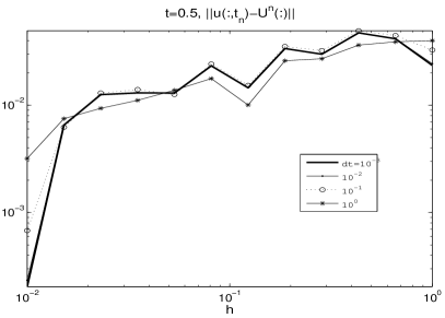
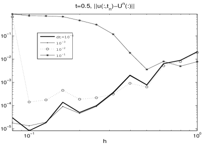
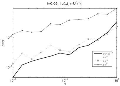
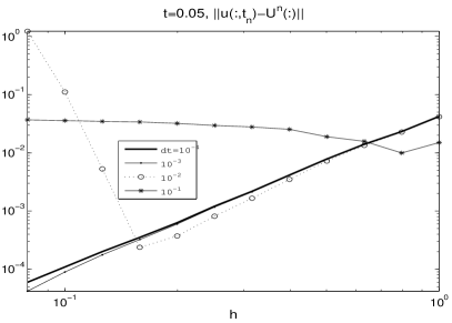
Figure 6: Here we present the error $\|u(:,t_{n})-U^{n}(:)\|$ estimated by the explicit scheme (right two) and the explicit-implicit (left two). Here in the bottom Figures we consider $J(x)=e^{-|x|}$, $u_{0}(x)=e^{-|x|}$; in the top Figures we consider $u_{0}(x)=\sqrt{\frac{10}{\pi}}e^{-10x^{2}}$, $J(x)=\sqrt{\frac{1}{\pi}}e^{-x^{2}}$

5 Accuracy of the semidiscrete approximation

Here we study the accuracy of the scheme (7). Applying the discrete Fourier transform on (7)

$$\tilde{U}_{t}(\xi,t)=\tilde{q}(\xi)\tilde{U}(\xi,t)$$ (34)

where $\xi\in\left[-\frac{\pi}{h},\frac{\pi}{h}\right]$ and

$$\tilde{q}(\xi)=\sqrt{2\pi}\left(\tilde{J}(\xi)-\tilde{J}(0)\right)-\frac{4}{h^{2}}\sin^{2}{\frac{h\xi}{2}}+\frac{i}{h}\sin({h\xi})-1$$

and thus

$$\tilde{U}(\xi,t)=e^{\tilde{q}(\xi)t}\tilde{U}_{0}(\xi).$$ (35)

Applying the inverse Fourier transform to (35)

$$U_{m}(t)=\frac{1}{\sqrt{2\pi}}\int_{-\frac{\pi}{h}}^{\frac{\pi}{h}}e^{imh\xi}e^{\tilde{q}(\xi)t}\tilde{U}_{0}(\xi)d\xi.$$ (36)

We interpolate $U_{m}(t)$ defined in (36) by [19]

$$\mathcal{S}U(x,t)=\frac{1}{\sqrt{2\pi}}\int_{-\frac{\pi}{h}}^{\frac{\pi}{h}}e^{ix\xi}e^{\tilde{q}(\xi)t}\tilde{U}_{0}(\xi)d\xi.$$

Similar to the Theorem 3 (using (21)),

$$u(x,t)-\mathcal{S}U(x,t)=\frac{1}{\sqrt{2\pi}}\int_{|\xi|\leq\frac{\pi}{h}}e^{ix\xi}\left(e^{\hat{q}(\xi)t}\hat{u}_{0}(\xi)-e^{\tilde{q}(\xi)t}\tilde{U}_{0}(\xi)\right)d\xi$$

$$+\frac{1}{\sqrt{2\pi}}\int_{|\xi|\geq\frac{\pi}{h}}e^{ix\xi}e^{\hat{q}(\xi)t}\hat{u}_{0}(\xi)d\xi.$$ (37)

Theorem 5.

If $J$, and $\hat{J}$ satisfy the assumptions H1 - H6 and $u_{0}\in H^{\sigma}(\mathbb{R})$ with $\sigma>\frac{1}{2},$ then there exist constants $C_{1}(h),$ $C_{3}(\sigma)$ such that

$$\|u(x,t)-\mathcal{S}U(t)\|\leq tC_{1}(h)\|u_{0}\|+C_{2}h\|u_{0}\|_{H^{2}(\mathbb{R})}^{2}+C_{3}(\sigma)h^{\sigma}\|u_{0}\|_{H^{\sigma}(\mathbb{R})},$$

where (7) is a semidiscrete approximation to the IDE (6).

Proof.

We have

$$\|u(\cdot,t)-\mathcal{S}U(\cdot,t)\|^{2} = \int_{-\infty}^{\infty}{\left|u(\cdot,t)-\mathcal{S}U(\cdot,t)\right|}^{2}dx$$ (38)

$$\leq \frac{1}{\sqrt{2\pi}}\int_{|\xi|\leq\frac{\pi}{h}}\left|e^{\hat{q}(\xi)t}\hat{u}_{0}(\xi)-e^{\tilde{q}(\xi)t}\tilde{U}_{0}(\xi)\right|^{2}d\xi$$

$$+\frac{1}{\sqrt{2\pi}}\int_{|\xi|\geq\frac{\pi}{h}}\left|\hat{u}_{0}(\xi)\right|^{2}d\xi$$

since by Lemma 1 $Real(\hat{q})\leq 0.$ Similar to the analysis of the full discrete approximation the first part of the right-hand side of (38) can be written as

$$\frac{1}{\sqrt{2\pi}}\int_{|\xi|\leq\frac{\pi}{h}}\left|e^{\hat{q}(\xi)t}\hat{u}_{0}(\xi)-e^{\tilde{q}(\xi)t}\tilde{U}_{0}(\xi)\right|^{2}d\xi$$

$$\leq \frac{2}{\sqrt{2\pi}}\int_{|\xi|\leq\frac{\pi}{h}}\left|e^{\hat{q}(\xi)t}-e^{\tilde{q}(\xi)t}\right|^{2}|\hat{u}_{0}(\xi)|^{2}d\xi+\frac{2}{\sqrt{2\pi}}\int_{|\xi|\leq\frac{\pi}{h}}\left|\sum_{j\neq 0}\hat{u}_{0}\left(\xi+\frac{2\pi j}{h}\right)\right|^{2}d\xi.$$

We have

$$\left|e^{\hat{q}(\xi)t}-e^{\tilde{q}(\xi)t}\right|\leq t|\hat{q}(\xi)-\tilde{q}(\xi)|$$

since $real(\tilde{q}(\xi))\leq 0\quad\mbox{and}\quad real(\hat{q}(\xi))\leq 0.$ Now

$$\hat{q}(\xi)-\tilde{q}(\xi) = \sqrt{2\pi}\sum_{j=-\infty,j\neq 0}^{\infty}\left(\hat{J}\left(\xi+\frac{2\pi j}{h}\right)-\hat{J}\left(\frac{2\pi j}{h}\right)\right)$$

$$+\left(\xi^{2}-\frac{4}{h^{2}}\sin^{2}(\frac{h\xi}{2})\right)+\left(-i\xi+\frac{i\sin(h\xi)}{h}\right)$$

$$= \sqrt{2\pi}\sum_{j=-\infty,j\neq 0}^{\infty}\left(\hat{J}\left(\xi+\frac{2\pi j}{h}\right)-\hat{J}\left(\frac{2\pi j}{h}\right)\right)+C_{2}h^{2}\xi^{4}+\mathcal{O}((h\xi)^{5}).$$

Thus

$$|\hat{q}(\xi)-\tilde{q}(\xi)| \leq C(h)+C_{2}h^{2}\xi^{4},$$

and $C(h)=2\hat{J}(\frac{\pi}{h})$ as $h\rightarrow 0$. Now

$$\int_{|\xi|\leq\frac{\pi}{h}}\left|e^{\hat{q}(\xi)t}-e^{\tilde{q}(\xi)t}\right|^{2}|\hat{u}_{0}(\xi)|^{2}d\xi \leq t^{2}\int_{|\xi|\leq\frac{\pi}{h}}\left|\hat{q}(\xi)-\tilde{q}(\xi)\right|^{2}|\hat{u}_{0}(\xi)|^{2}d\xi$$

$$\leq t^{2}C(h)^{2}\|u_{0}\|^{2}+C^{2}h^{2}\|u_{0}\|_{H^{2}(\mathbb{R})}^{2},$$

gives

$$\int_{|\xi|\leq\frac{\pi}{h}}\left|e^{\hat{q}(\xi)t}-e^{\tilde{q}(\xi)t}\right|^{2}|\hat{u}_{0}(\xi)|^{2}d\xi\leq t^{2}C^{2}(h)\|u_{0}\|^{2}+C_{2}t^{2}h^{2}\|u_{0}\|_{H^{2}(\mathbb{R})}^{2}.$$ (39)

Thus applying (26),(27) and (39), (38) takes the form

$$\|u(x,t)-\mathcal{S}U(t)\|\leq tC_{1}(h)\|u_{0}\|+C_{2}h\|u_{0}\|_{H^{2}(\mathbb{R})}^{2}+C_{3}(\sigma)h^{\sigma}\|u_{0}\|_{H^{\sigma}(\mathbb{R})}$$ (40)

for some $C_{1}$, $C_{2}$, $C_{3}$ for all $u_{0}\in H^{\sigma}(\mathbb{R})$ with $\sigma>\frac{1}{2}.$ ∎

6 Summary and conclusions

In this study, we consider a linear partial integro-differential operator (PIDO) that comes in modeling financial engineering problems as well as in modeling various scientific problems. We study a few finite difference schemes (FDSs) for European style options with a jump-diffusion term (the PIDO). In the first part of the study we introduce several preconditioned linear system solvers for the full discrete equivalent of the model. We observe that all the preconditioned solvers are very efficient, and the multigrid solver is way better than the wavelet diagonal preconditioned solver and the Fourier sine preconditioned solvers. In fact, a one $v-$cycled Multigrid solver is several times faster than the other two. The implementation costs for the sine and the wavelet preconditioning are relatively higher than that of the multigrid technique. So we conclude that a multigrid method can be used to speed up the computation of the finite dimensional (full discrete) PIDE model. Here we also conclude that the explicit implicit scheme outperforms the implicit scheme in terms of computational costs.

Here, in the second part of this study, we analyze the stability and the accuracy of two different finite difference schemes. While analyzing the stability and the accuracy of the finite difference schemes (an explicit scheme as well as an explicit implicit scheme) we notice that the schemes are conditionally stable (under some reasonable restrictions imposed on the kernel function). The explicit implicit scheme is faster than that of the explicit scheme as well as the implicit scheme, which agrees with the properties of the time and the space discretizations of the PIDE we consider in this study. We establish some bounds of the error in such full discrete as well as semi-discrete schemes.

Here we analyze the model in one space dimension only. Preconditioners can be employed to speed up the computational process for the full discrete model, specially for two and three space dimensional domains as well as preconditioned solvers along with higher order multi-step schemes may be better options to think of, and that leaves as future research directions.

References

- [1] Q. Alfio, R. Sacco, and F. Saleri. Numerical Mathematics. Springer, 2000.
- [2] S. K. Bhowmik. Numerical approximation of a nonlinear partial integro-differential equation. PhD thesis, Heriot-Watt University, Edinburgh, UK, April, 2008.
- [3] S. K. Bhowmik. Numerical approximation of a convolution model of dot theta-neuron networks. Applied Numerical Mathematics, 61:581–592, 2011.
- [4] S. K. Bhowmik and C. C. Stolk. Preconditioners based on windowed fouerier frames applied to elliptic partial differential equations. Journal of Pseudo-Differential Operators and Applications, 2(3):317–342, April 2011.
- [5] W. L. Briggs. Multigrid Tutorial. SIAM, Pennsylvania, 1987.
- [6] K. Chen. Matrix Preconditioning Techniques and Applications. Cambridge University Press, 2005.
- [7] R. Cont and E. Voltchkova. A finite difference scheme for option pricing in jump diffusion and exponential levy models. SIAM J. NUMER. ANAL., 43(4):1596–1626, 2005.
- [8] S. Coombes, G. J. Lord, and M. R. Owen. Waves and bumps in neuronal networks with axo-dendritic synaptic interactions. SIAM Journal., 3(October), 2002.
- [9] D. J. Duffy. Finite Difference Methods for Financial Engineering, A Partial Differential Equation Approach. Wiley Finance, John Wiley and Sons, 2006.
- [10] D. B. Duncan, M. Grinfeld, and I. Stoleriu. Coarsening in an integro-differential model of phase transitions. Euro. Journal of Applied Mathematics, 11:511–523, 2000.
- [11] L. C. Evans. Partial Differential Equations. AMS, 1998.
- [12] F. Fiorani. Option Pricing Under the Variance Gamma Process. PhD thesis, University of Trieste, 2009.
- [13] G. H. Golub and C. F. V. Loan. Matrix Computations. Third edition, The Johns Hopkins University Press, Baltimore and London, 1996.
- [14] Y. Guo and C. C. Chow. Existence and stability of standing pulses in neural networks:—existence. SIAM J. Applied Dynamical Systems, 4(2):217–248, 2005.
- [15] K. Maleknejad. A comparison of fourier extrapolation methods for numerical solution of deconvolution. New York Journal of Mathematics, 183:533–538, 2006.
- [16] S. Mallat. A Wavelet Tour of Signal Processing. Elsevier, 2009.
- [17] J. Medlock and M. Kot. Spreading disease: integro-differential equations old and new. Mathematical Biosciences, 184:201–222, 2003.
- [18] C. C. Stolk. A preconditioner for the helmholtz equation based on adaptive phase space tiling. Xrive, 2010.
- [19] J. C. Strikwerda. Finite Difference Schemes and Partial Differential Equations. Wadsworth and Brooks, Cole Advanced Books and Software, Pacific Grove, California, 1989.
- [20] L. N. Trefethen. Spectral Methods in Matlab. SIAM, Philadelphia, 2000.
- [21] U. Trottenberg, C. W. Oosterlee, and A. Schuller. Multigrid. Academic Press, 2001.
- [22] K. Urban. Wavelet Methods for Elliptic Partial Differential Equations. Oxford University Press, 2009.
- [23] J. S. Walker. Fast Fourier Transforms. Second edition, CRC press, Boca Raton, New York, London, Tokyo, 1996.