Observations of four glitches in the young pulsar J1833$-$1034 and study of its glitch activity

Abstract

We present the results from timing observations with the GMRT of the young pulsar J1833$-$1034, in the galactic supernova remnant G21.5$-$0.9. We detect the presence of 4 glitches in this pulsar over a period of 5.5 years, making it one of a set of pulsars that show fairly frequent glitches. The glitch amplitudes, characterized by the fractional change of the rotational frequency, range from $1\times 10^{-9}$ to $7\times 10^{-9}$, with no evidence for any appreciable relaxation of the rotational frequency after the glitches. The fractional changes observed in the frequency derivative are of the order of $10^{-5}$. We show conclusively that, in spite of having significant timing noise, the sudden irregularities like glitches detected in this pulsar can not be modeled as smooth timing noise. Our timing solution also provides a stable estimate of the second derivative of the pulsar spin-down model, and a plausible value for the braking index of 1.857, which, like the value for other such young pulsars, is much less than the canonical value of 3.0. PSR J1833$-$1034 appears to belong to a class of pulsars exhibiting fairly frequent occurrence of low amplitude glitches. This is further supported by an estimate of the glitch activity parameter, $A_{g}~{}=~{}1.53\times 10^{-15}$ $s^{-2}$, which is found to be significantly lower than the trend of glitch activity versus characteristic age (or spin frequency derivative) that a majority of the glitching pulsars follow. We present evidence for a class of such young pulsars, including the Crab, where higher internal temperature of the neutron star could be responsible for the nature of the observed glitch activity.

1 Introduction

Beside the basic, smooth spin-down of the neutron star due to the electromagnetic torque mechanism, pulsar timing studies also reveal the presence of irregularities in the rotation of the star, mainly of two kinds : timing noise, which is characterized by continuous, random fluctuations in the rotation rate; and glitches, which are sudden increases in the rotation rate. These spin-up events are superposed on the long-term spin-down of the pulsar, and manifest themselves as sudden early arrival of the pulses. A recent work by (Espinoza et al., 2011) reports a total of 315 glitches observed in 102 pulsars. The magnitude of the change in rotation frequency, $\nu$, during a glitch is typically in the range $10^{-10}$ $<$ $\Delta\nu/\nu$ $<$ $10^{-6}$, and the fractional increment in the spin-down rate, $\Delta\dot{\nu}/\dot{\nu}$, is in the range $10^{-5}$ to $10^{-2}$.

The most plausible explanation for the sudden spin-up is the irregular flow of angular momentum from the faster rotating superfluid interior to the more slowly rotating solid crust of the neutron star as it slows down (Lyne et al., 1995). The current unified model for glitches is based on the superfluidity of the neutrons in a neutron star. The rotating superfluid in the neutron star carries angular momentum, by forming quantized vortices. The spacing between the vortices is negligible compared to the radius of the neutron star. On the macroscopic scale, the flow pattern looks like uniform rotation. These quantized vortices in the neutron superfluid in the inner crust can get pinned to the lattice of heavy neutron-rich nuclei. The pinning is possible because the effective width of the vortex core is less than or comparable to the lattice spacing of the nuclei. The pinning force is related to the energy gain when vortices are pinned to the lattice. The vortices stay pinned in this manner until a stronger force unpins them from the lattice sites. These pinned vortices in the crustal nuclei are rotating slower than the surrounding superfluid. Due to this differential velocity, magnus forces that act radially outward cause sudden unpinning and migration of vortices, which results in the transfer of angular momentum from the superfluid to the crust. This gives rise to a sudden speed-up of the solid crust, which manifests as a glitch in the timing behaviour of the pulsar. Anderson and Itoh (1975) were the first to make this connection between sudden unpinning of vortices and pulsar glitches. In the unpinned state, the superfluid moment of inertia is not coupled to the crust, hence the effective moment of inertia of the crust decreases, which in-turn increases the spin-down rate. Between glitches, the vortex lines undergo a slow, thermally activated process, called vortex creep. The post-glitch relaxation is a process of recoupling of the vortices to another steady (pinned) state. Once the moment of inertia recovers due to this recoupling via repinning, the original extrapolated spin-down rate is restored. Thus, the observed sudden increase in the rotation rate, followed by exponential relaxation back to the extrapolated pre-glitch rotation rate, provides a useful probe of the neutron star interior.

The pulsar J1833$-$1034 was independently discovered at the GMRT (Gupta et al., 2005) and at Parkes (Camilo et al., 2006) and is associated with the galactic supernova remnant (SNR) G21.5$-$0.9. This pulsar has quite a high spin-down luminosity that is amongst the top ten of all the known pulsars in our Galaxy. The flux density measured at radio wavelengths is very low $-$ the estimated mean flux density from the observations at 610 MHZ is 0.65 mJy (Gupta et al., 2005). With a period of 61.86 ms and a period derivative of 2.02$\times$10^-13 s/s, it has a characteristic age, $\tau_{c}$ $\approx$ 4.8 kyr (Camilo et al., 2006), which makes it a fairly young pulsar. Existing studies indicate that younger pulsars are more likely to show glitches. About half of all known pulsars with $\tau_{c}$ less than 3$\times$10⁴ have exhibited glitches, but this fraction is much lower for the older population (Yuan et al., 2010). PSR J1833$-$1034 is thus a good candidate for the study of glitches. In this paper we report the detection of multiple glitches from this pulsar using timing observations carried out at the GMRT at 610 MHz, and present a detailed study of its glitch activity. We also provide refined estimates of the timing parameters for this pulsar, including an estimate of the braking index. In Section 2 we explain the observations and data analysis techniques. Section 3 describes the detected glitches and their modeling in detail. In Section 4 we discuss the significance of our results. Summary and future scope are presented in section 5.

2 Observations and data analysis

The GMRT is a multi-element aperture synthesis telescope consisting of 30 antennae, each of 45 m diameter, spread over a region of 25 km diameter (Swarup et al., 1997). Though designed to function primarily as an aperture synthesis telescope, the GMRT can also be used as an effective single dish in an array mode by adding the signals from individual dishes, either coherently or incoherently (Gupta et al., 2000), for studying compact objects like pulsars. The radio signals at the observing frequency band, from both polarizations of the 30 dishes, are eventually converted to baseband signals of 16 MHz or 32 MHz bandwidth, which are then sampled at Nyquist rate. These digitised signals are delay corrected and then Fourier Transformed in a FX correlator to get spectral information. After fringe derotation, these dual polarization spectral voltage samples from all the antennae are added coherently in the GMRT Array Combiner (GAC), to produce the phased array outputs for each polarization. These are then converted to intensity, integrated to the desired time constant and recorded on disk for off-line processing. The data are time-stamped using a minute pulse signal, derived from the observatory’s GPS receiver, which is embedded in the data stream.

The timing observations described here were carried out in the total intensity phased array mode at 610 MHz. In this mode of operation, the array needs to be phased up before observing the target pulsars. This is achieved by recording the correlator data for a point source calibrator, solving for the antenna based gains and phases from these, and applying the phases as corrections to the output of the Fourier Transform stage of the correlator. The array remains phased for up to a few hours and dephases due to slow changes in instrumental and ionospheric phases. When this happens, one needs to rephase the array to proceed with further observations.

Table 1: Main parameters for the two pulsars observed, at 610 MHz with a bandwidth of 16 MHz, with a typical cadence of 10 days.

PSR	Period	Mean flux at	Integration	$N_{p}$	$(S/N)_{exp}$
	(ms)	610 MHz(mJy)	time (min)
B1855+09	5.36	16.8†	5	55970	177
J1833-1034	61.86	0.65‡	90	87293	32

${\dagger}$ extrapolated flux using the catalogued values at 400 and 1400 MHz.

${\ddagger}$ Gupta et al. (2005)

$N_{p}$ is number of pulses accumulated in the integration time.

$(S/N)_{exp}$ is the expected S/N for the 610 MHz profile at any epoch.

Timing observations for PSR J1833$-$1034 were started around mid-2005, shortly after its discovery at the GMRT. In the beginning, after the initial, closely spaced observations that are needed to obtain the timing solution for a newly discovered pulsar, the observations were somewhat random and sparse in time. Since the occurrences of glitches are unpredictable and their relaxation timescales can be quite short, regular monitoring is important for detection and study of the glitches. From mid-2007, after the possible detection of the first glitch from this pulsar, a regular timing program was started, with observations roughly about 10 days apart, except for the GMRT maintenance intervals. Each observing epoch has a 90 min long scan on PSR J1833$-$1034, and a shorter scan of 5 min on PSR B1855$+$09, which acts as a control pulsar for validating the data quality and reliability of the time-of-arrival (TOA) values from the newly established GMRT timing pipeline. The final data for each scan are total intensity values for each of 256 spectral channels (across a 16 MHz bandwidth), recorded with a sampling interval of 0.256 ms. The main observing parameters for a typical epoch are summarized in Table 1.

In the off-line processing, the recorded multi-channel total intensity data are first dedispersed to remove the effect of interstellar dispersion on the pulse shape. The dedispersed time series data are then synchronously folded using the topocentric pulsar period, obtained from the best existing model parameters (barycentric) for the concerned pulsar, after correcting for the observing time and location. The UTC corresponding to the middle of the observing session is used as the reference point for that particular epoch and it is derived from analysis of the GPS pulse signal embedded in the data. The predicted topocentric periods are calculated using “polyco” files produced by the pulsar timing program TEMPO . For the control pulsar, the barycentric model parameters were taken from the ATNF pulsar catalog ; for J1833$-$1034, these were obtained from the initial epochs of observations and refined at successive epochs, as required. The topocentric TOAs at each epoch are obtained by cross-correlating the average profile at that epoch with the highest signal-to-noise (S/N) profile from all the epochs used as a template. These are then converted to solar system barycentric TOAs using the Jet Propulsion Laboratory DE200 solar system ephemeris (Standish, 1982) inside TEMPO. To illustrate the quality of the profiles, Fig. 1 shows the highest S/N profile (which is used as the template), as well as a typical average profile (whose S/N is close the median value from profiles of all epochs). For the timing analysis using TEMPO, we have used these topocentric TOAs along with the uncertainties related to the S/N of the profiles. The tiny uncertainty of the TOA of the reference epoch is artificially increased to make it close to the median value.

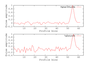
Figure 1: Highest signal-to-noise ratio profile (top panel) and typical average profile (bottom panel) for PSR J1833$-$1034. The highest signal-to-noise ratio is 22, whereas the typical average profile has a signal-to-noise ratio of 10.

At the solar system barycentre, the time evolution of the rotational phase of a solitary pulsar is well-approximated by a polynomial of the form (Manchester and Taylor, 1977)

$$\phi_{m}(t)=\phi_{0}+\nu(t-t_{0})+\frac{1}{2}\dot{\nu}(t-t_{0})^{2}+\frac{1}{6}\ddot{\nu}(t-t_{0})^{3}$$ (1)

where $\phi_{0}$ is the reference phase at time $t_{0}$; $\nu$, $\dot{\nu}$ and $\ddot{\nu}$ are the pulsar rotational frequency and its derivatives. TEMPO attempts to minimize the deviations between the observed and model rotational phases using $\chi^{2}$ minimization. Timing irregularities are seen as slow, large changes in the residuals $\phi$ $-$ $\phi_{m}$, where $\phi$ is the measured phase and $\phi_{m}$ is the model phase.

For a glitch, there is a sudden change in the phase residuals, modeled by an abrupt jump in the frequency and its derivative, followed by a relaxation process. The frequency perturbation due to a glitch can be described as (Yuan et al., 2010)

$$\Delta\nu(t)=\Delta\nu_{p}+\Delta\dot{\nu_{p}}t+\Delta\nu_{d}e^{-t/\tau_{d}}$$ (2)

$$\Delta\dot{\nu}(t)=\Delta\dot{\nu_{p}}+\Delta\dot{\nu_{d}}e^{-t/\tau_{d}}$$ (3)

where $\Delta\nu$ and $\Delta\dot{\nu}$ are the changes in the pulse frequency and its derivative, relative to the pre-glitch model; $\Delta\nu_{p}$ and $\Delta\dot{\nu_{p}}$ are the persistent change in rotational frequency and its derivative; $\Delta\nu_{d}$ is the amplitude of the exponentially decaying part of the jump in rotational frequency (and $\Delta\dot{\nu_{d}}$ is the corresponding value for the frequency derivative), with a relaxation time constant $\tau_{d}$. The total frequency change at the time of the glitch is then given by

$$\Delta\nu_{g}=\Delta\nu_{p}+\Delta\nu_{d}$$ (4)

The instantaneous change in $\dot{\nu}$ at the glitch is given by,

$$\Delta\dot{\nu_{g}}=\Delta\dot{\nu_{p}}+\Delta\dot{\nu_{d}}$$ (5)

3 Results

We first discuss the timing results for the control pulsar and then present the results from the timing analysis of the target pulsar J1833$-$1034, using GMRT data spanning 30th July 2005 to 11th Jan 2011. The post-fit residuals obtained from the phase connected timing solution for the control pulsar B1855$+$09 (shown in Fig. 2) over the full data span of 52 epochs, yield a root-mean-square (rms) value of 15 $\mu$s. This is more than the theoretical, expected value ($\sigma_{th}$) of 3 $\mu$s, which is based on the expected S/N of 177 given in Table 1, and using $\sigma_{TOA}$ $\simeq$ $\frac{W}{S/N}$ (where $W$ is the pulse width and $S/N$ is the expected signal-to-noise ratio of the average profiles). However, it matches well with the value expected for the achieved S/N (which has a maximum value of 35 in all the observing epochs). Nevertheless, our final 610 MHz timing residuals for PSR B1855$+$09 are worse off by factor of 5 in rms from the 1420 MHz results obtained by Hobbs et al. (2006). In addition to signal to noise limitations, there can be effects of interstellar weather that can reduce the accuracy of the TOAs : the pulse arrival time at each epoch can have extra deviations due to propagation effects in the interstellar medium, which will be larger at the lower frequency. These results verify, to first order, the proper working of the pulsar timing set-up at the GMRT.

In order to check for any low-level systematic effects in the timing residuals for this control pulsar, we investigated the changes in the rms value when adjacent residuals are averaged. For truly white-noise residuals, this rms should decrease as the square root of the number of residuals averaged. Fig. 3 shows the results for this on a log-log plot, where the data points are found to match quite well with a slope of $-$0.5 (green dashed line). The over-all post-fit residuals thus exhibit a white-noise behaviour and are likely free from any systematics. The averaging of post-fit residuals over 166 days (10 TOAs) achieves a rms of 3 $\mu$s for B1855$+$09, which implies a long-term timing stability of 1 part in 4$\times 10^{12}$. The above results for the control pulsar establish the basic fidelity of the timing pipeline for the GMRT.

For PSR J1833$-$1034, since the S/N is typically significantly lower than for the control pulsar, to check the data quality for timing purposes we show the distribution of TOA errors in Fig. 4. The bulk of the values are clustered in the range of 100 to 300 $\mu$s, with a small tail of larger values. This skew in the distribution is due to degradation of S/N at some epochs, possibly due to fading caused by interstellar scintillation. However, the achieved TOA uncertainties are still good enough to detect changes in the residuals of the order of several milliseconds due to the occurrence of glitches.

Figure 2: Timing residuals for the control MSP B1855$+$09, which show a rms $\sim$ 15 $\mu$s.

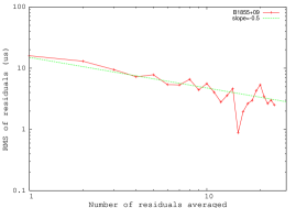
Figure 3: RMS of residuals versus number of consecutive residuals averaged, for the PSR B1855$+$09. Green dashed lines indicate the expected slope of $-$0.5 for uncorrelated residuals.

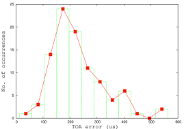
Figure 4: Distribution of TOA errors for PSR J1833$-$1034.

Figure 5: Timing residuals for the target pulsar PSR J1833$-$1034 from the first 1.5 years of data, prior to the first detected glitch at $\sim$ 2007.2.

Starting with the initial timing observations for PSR J1833$-$1034, we are able to build up a phase-connected timing solution (shown in Fig. 5), till the epoch of 2007.2. From this 1.5 year data span, we obtain a fairly good timing model for this pulsar, including a second frequency derivative (see the first row of Table 2), and the rms of the residuals is around 174 $\mu$s. The reference epoch (MJD) for these measurements is set to the epoch which is mid-point of our full data span (i.e. MJD of 54575), for better comparison with the later models. The pulsar position used in the timing model is the one determined from the Chandra observations (Camilo et al., 2006). The position derived from our timing solution of 1.5 years of phase-connected residuals is within the 3$\sigma$ error bars of this X-ray position. We derive a braking index ($n$ $=$ $\nu\ddot{\nu}$/$\dot{\nu}^{2}$ ) of 2.168(8) for this pulsar from this initial data span (see last column of Table 2).

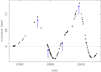
Figure 6: Residuals from the full 5.5 yrs of data without modeling of any glitch event, showing strong signature of timing noise, as well as evidence for glitches $-$ these are typically seen as sudden negative change in the slope of the residuals, and the suspected locations are indicated by arrows. The detection and modeling of these glitches are explained in detail in the text, and illustrated in Figs 8, 8, 10 & 10.

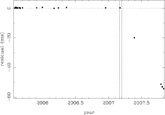
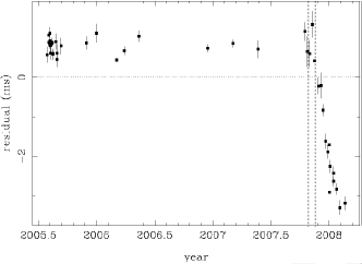
Figure 7: Timing residuals illustrating the first glitch event at $\sim$ 2007.2. This initial model is obtained from fitting $\nu$, $\dot{\nu}$ and $\ddot{\nu}$ to TOAs from 2005.5 up to the suspected epoch of the glitch. The final model yields a glitch with $\Delta\nu_{g}$/ $\nu$ of $3.34\times 10^{-9}$, localised in time to the interval marked by the dotted lines.

Figure 8: Timing residuals illustrating the second glitch event at $\sim$ 2007.9. This initial model is obtained from fitting $\nu$, $\dot{\nu}$ and $\ddot{\nu}$ and the glitch model for the first glitch, to TOAs from 2005.5 up to the suspected epoch of the glitch. The final model yields a glitch with $\Delta\nu_{g}$/ $\nu$ of $1.00\times 10^{-9}$, localised in time to the interval marked by the dotted lines.

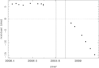
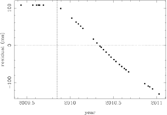
Figure 9: Timing residuals illustrating the third glitch event at $\sim$ 2008.8. This initial model is obtained from fitting $\nu$ & $\dot{\nu}$ over the first 130 days shown here, with $\ddot{\nu}$ held constant at the value obtained from the fit to the first 1.5 years of data. The final model yields a glitch with $\Delta\nu_{g}$/ $\nu$ of $1.6\times 10^{-9}$, localised in time to the interval marked by the dotted lines.

Figure 10: Timing residuals illustrating the fourth glitch event at $\sim$ 2009.9. This initial model is obtained from fitting $\nu$ & $\dot{\nu}$ over the first 152 days shown here, with $\ddot{\nu}$ held constant at the value obtained from the fit to the first 1.5 years of data. The final model yields a glitch with $\Delta\nu_{g}$/ $\nu$ of $6.9\times 10^{-9}$, localised in time to the interval marked by the dotted lines.

Table 2: Rotational parameters for PSR J1833$-$1034 from different timing solutions. The first row is for the timing solution from the initial 1.5 years of data, before the first detected glitch. The second row is for the full 5.5 yrs of data, without inclusion of any glitch models. The third row is for the full 5.5 yrs of data, with glitch models fixed to the values derived from the piecemeal modeling of the glitches. The last row is for the solution from the final global fit, including all four glitches (2 free parameters each, with glitch epochs fixed to the values obtained from the piecemeal fittings), and four frequency derivatives. All errors are 1$\sigma$ values.

No of glitches	Ref Epoch	Data span	No. of	$\nu$	$\dot{\nu}$	$\ddot{\nu}$	Residual	Braking
fitted	(MJD )	MJD	TOAs	($s^{-1}$)	($10^{-11}s^{-2}$)	($10^{-22}s^{-3}$)	(ms)	Index
$-$	54575	53581$-$54164	22	16.159357125(2)	$-$5.275017(9)	3.73(1)	0.174	2.168(8)
$-$	54575	53581$-$55572	94	16.15935713057(2)	$-$5.27507199(3)	3.6006(2)	15.4	2.0891(1)
$4$	54575	53581$-$55572	94	16.15935711448(2)	$-$5.27507291(3)	3.6232(2)	2.20	2.1041(1)
$4$	54575	53581$-$55572	94	16.15935711336(3)	$-$5.2751130(1)	3.197(1)	0.512	1.8569(6)

Fig. 6 shows the timing residuals for the full data set (94 epochs spanning 5.5 years) for this pulsar, relative to a simple slow-down model including the pulsar spin frequency and its first two derivatives. The best fit model parameters from this are listed in the second row of Table 2. The residuals, with a relatively large rms of 15.4 ms, are clearly dominated by non-random, low frequency timing noise effects. The amplitude of this timing noise is a strongly increasing function of the length of the data span. The effect of this timing noise was probably not detected for the initial data span of 1.5 years, as the fitting of the spin-frequency and its two derivatives can mask most of the low-frequency trends. In these timing noise dominated residuals of Fig. 6, the presence of glitches can be distinguished by sudden changes in the slope of the curve. Clear events are seen at 2007.2 and 2009.9, and less likely ones at 2007.9 and 2008.8, all of which are marked by arrows in Fig. 6.

The presence of a glitch is confirmed by taking relatively shorter stretches of data around the suspected glitch event, and doing a local timing fit to the TOAs, starting with a model for the data prior to the glitch. Sudden, systematic deviation of the residuals from a smooth behaviour is taken as the signature of the occurrence of a glitch (as seen in Figs 8, 8, 10 & 10). Detailed modeling is then carried out to estimate the glitch epoch, and the changes in frequency and frequency derivative at the glitch. The best possible value of the glitch epoch is estimated by minimising the phase increment required to obtain a phase-connected solution over the interval around the glitch epoch (Janssen et al., 2006). The measurement uncertainty of the glitch epoch is obtained from the corresponding 3$\sigma$ limit of the glitch phase increment parameter.

Starting with an initial timing model having $\nu$, $\dot{\nu}$ and $\ddot{\nu}$, we find that the first glitch (Fig. 8) occurred at MJD $=$ 51469 ($\pm$ 7), with a fractional change in the rotational frequency (${\Delta\nu_{g}}/{\nu}$) of 3.34$\times 10^{-9}$. The modeling for this glitch includes 26 TOAs observed over 824 calender days, of which there are 236 days of data after the glitch event. Fig. 8 shows the second glitch event, which is best fit by a fractional increase in rotational frequency of 1.00$\times 10^{-9}$ at MJD $=$ 54423 ($\pm$ 9). As we have a fairly good timing model for the first 1.5 years (including the first glitch event), without any timing noise effects, the pre-glitch interval for this second glitch includes all of these TOAs over 842 calender days, with a pre-fit model of $\nu$, $\dot{\nu}$, $\ddot{\nu}$ and the derived parameters of the first glitch. There is a third glitch (Fig. 10) detected at MJD $=$ 54750 ($\pm$ 15) with a fractional change in the rotational frequency of 1.6$\times 10^{-9}$. The last glitch event (Fig. 10) observed at MJD $=$ 55142 ($\pm$ 2) yields a fractional change in the rotational frequency of 6.9$\times 10^{-9}$. In order to minimse the effects of timing noise, the pre-glitch interval for the third glitch includes TOAs over 130 days and the fourth glitch includes TOAs over 152 days, with the pre-fit model having $\nu$, $\dot{\nu}$ & $\ddot{\nu}$. But since the pre-fit data span over smaller intervals, the fit uses $\nu$, $\dot{\nu}$ as free parameters, with $\ddot{\nu}$ kept constant to the value derived from the initial 1.5 yrs of data. Inclusion of TOAs over larger spans increases the influence of timing noise, where the residuals depart from the simple spin-down model with $\nu$, $\dot{\nu}$ and $\ddot{\nu}$, making it harder to detect the glitches accurately. There are also small changes in slow-down rate, of the order of $10^{-5}$, observed at the glitch epochs. The new timing models, after inclusion of the glitch parameters, yield phase-connected timing residuals with rms values of 177 $\mu$s, 216 $\mu$s, 227 $\mu$s and 1.5 $m$s respectively, for the four cases.

It is sometimes possible that, for data that are relatively sparsely sampled and have significant amount of timing noise (both of which are somewhat true for the present case), there can be large deviations in residuals with respect to the basic spin-down model of $\nu$, $\dot{\nu}$ & $\ddot{\nu}$, which $\it may$ mimic glitch-like behaviour. In order to discriminate between the effect of timing noise and genuine glitches, we investigated the pre-fit and post-fit residuals around the glitch epochs by fitting with higher frequency derivatives without inclusion of any glitch model. For example, for the case of TOAs spanning over the first 936 days (including glitch-1 and glitch-2), the rms for the post-fit residuals is 216 $\mu$s (shown in Fig. 11). The model includes two glitches and a spin-down model with $\nu$, $\dot{\nu}$ & $\ddot{\nu}$, which amount to 9 free parameters. The same span of TOAs can also be fitted with a model having $\nu$ and 8 frequency derivatives, without inclusion of any glitch models, which also amounts to 9 free parameters, as for the model with glitches. The post-fit residuals shown in Fig. 12, have a much larger rms value of 951 $\mu$s and also show large discontinuities, including at the glitch epoch. Similar effects were found for the data around the 3rd and 4th glitches. This illustrates the fact that some of the large TOA variations that we see for this pulsar, over and above the basic spin-down model, can not be satisfactorily explained with a model of timing noise characterised by higher order derivatives, but are better modeled with discrete glitch events.

Figure 11: Post-fit residuals after fitting for the first two glitches, for TOAs spanning the first 936 days. The rms is 216 $\mu$s.

Figure 12: Post-fit residuals (for TOAs spanning the first 936 days) after fitting with a model having $\nu$ and 8 frequency derivatives, without inclusion of any glitch models, which amounts to 9 free parameters, as for the model with glitches. The rms is 951 $\mu$s, and there are large deviations at the epoch of the first glitch.

Finally, to obtain a global model for the entire data span, we have compared the following three approaches : (i) taking the models for the 4 glitches obtained from the piecemeal fits to the individual glitches as fixed and then fitting for $\nu$, $\dot{\nu}$ & $\ddot{\nu}$ over the entire data span; (ii) a fit to the full data span using $\nu$ and up to 12 frequency derivatives (the maximum allowed by TEMPO) without any glitch models included; and (iii) a global fit for 4 glitches, $\nu$ and first four frequency derivatives, to achieve the same count of 13 free parameters as in case (ii) $-$ each glitch contributes 2 free parameters (spin-frequency increment and change in spin-down rate), as the glitch epochs are fixed to the values obtained during the piecemeal fittings, by minimising the phase increment at the glitch epoch. Case (i) gives the residuals shown in the middle panel of Fig. 13, with an rms of 2.2 ms, and fairly smooth behaviour with large swings, typical of timing noise. Results from this fit are given in the third row of Table 2. Case (ii) gives the residuals shown in the top panel of Fig. 13. Though the rms is 1.4 ms, the variations of the residuals show sudden, large jumps (as at the epoch of the first glitch) and also sharp, cuspy variations (as at the epoch of the 4th glitch). For case (iii), global fits with all 4 glitches (using the results from the piecemeal fits as the starting pre-fit model) and increasing number of frequency derivatives were tried, and the following was found : for 4 glitches plus $\nu$, $\dot{\nu}$ & $\ddot{\nu}$, the residuals are 1.2 ms and the behaviour is qualitatively similar to case (i); for the case of two more derivatives added to achieve the same number of 13 degrees of freedom as it was for the case (ii), the residuals (shown in the bottom panel of Fig. 13) reduce significantly to 0.5 ms and also the slow, large fluctuations typical of timing noise are noticeably suppressed. The glitch parameters are not very different from those obtained from the piecemeal fits. The results from this model are summarised in the 4th row of Table 2 and the final glitch parameters are given in Table 3.

From the above, we argue that the best timing model is that given by a global fit of 4 glitches and 5 spin frequency terms, which gives the best global fit to the data and reduces the residuals to a minimum. The attempt to fit the TOAs with a pure timing noise model having large number of derivatives does not give acceptable results : both for localised fits to data sets that span individual glitches, as well as for the global data set. For such cases, the rms of the residuals is larger and/or the residuals show uncharacteristically large, abrupt changes. We take the results from this fit as the final timing model for this data set. These results are summarised in the last row of Table 2 and in Table 3.

Now in order to measure the amount of timing noise present in this pulsar, we have used the definition given by Arzoumanian et al. (1994),

$$\Delta_{8}=log_{10}(\frac{1}{6\nu}|\ddot{\nu}|t^{3})$$ (6)

where the spin-frequency, $\nu$ and its second derivatives, $\ddot{\nu}$, are measured over a $t$ $=$ $10^{8}$ s interval. We have used first 3.16 years of data for PSR J1833$-$1034 to estimate the value of $\Delta_{8}$ as 0.5, which follows the correlation between timing noise and spin-down rate, i.e. the younger pulsars with larger spin-down rate exhibit more timing noise than older pulsars, seen by Arzoumanian et al. (1994) and later by Hobbs et al. (2010).

The value of the braking index determined from the final global fit is 1.8569(6). This braking index is much less than 3, which is in general agreement with the values obtained for other young pulsars having reliable estimates for this quantity. For example, for Crab pulsar, $n$ $=$ 2.509(1) (Lyne et al., 1988, 1993), for PSR J1846$-$0258, $n$ $=$ 2.65(1) (Livingstone et al., 2006), for PSR B0540$-$69, $n$ $=$ 2.140(9) (Livingstone et al., 2005), for PSR B1509$-$58, $n$ $=$ 2.837(1) (Kaspi et al., 1994) and for PSR J1119$-$6127, $n$ $=$ 2.684(2) (Weltevrede et al., 2011). A value of n $<$ 3 indicates that simple magnetic dipole model does not completely explain spin-down evolution of pulsars. Particle outflow in the pulsar wind can also carry away some of its rotational kinetic energy.

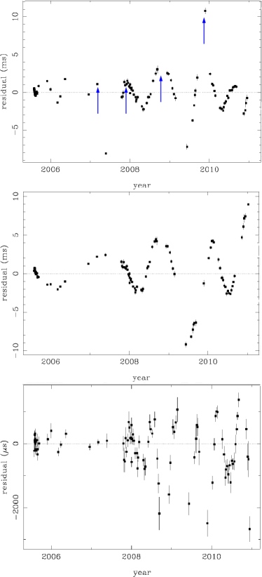
Figure 13: Timing residuals for PSR J1833$-$1034, for different types of global fits, all having the same number of 13 free parameters. The top panel shows residuals with 12 frequency derivatives fitted, without any glitch models. The suspected glitch epochs are marked by arrows. At the first, third and fourth glitch epochs there is clear evidence for discontinuities in the residuals. The middle panel shows residuals with a model of four glitches, derived from piecemeal fitting and two derivatives of pulsar spin-frequency. The presence of low-frequency timing noise is clearly seen in these residuals, which otherwise show a smooth behaviour. The bottom panel shows residuals obtained from a global fit of four glitch models and four frequency derivatives. The rms is significantly lower and the residuals are much more whitened in nature, indicating that this model gives the best global timing fit to this data set.

Table 3: The parameters of all the four glitches detected in PSR 1833$-$1034, as determined from a global fit to the timing data. The errors on the least significant digit are at 1$\sigma$ level.

Glitch epoch	Date	Fit span	$\frac{\Delta\nu_{g}}{\nu}$	$\frac{\Delta\dot{\nu}_{g}}{\dot{\nu}}$
(MJD)		(MJD)	($10^{-9}$)	($10^{-5}$)
54169 ($\pm$7)	5th Mar2007	53581$-$54405	3.11(5)	1.4(2)
54423 ($\pm$9)	12th Nov2007	53581$-$54517	1.09(6)	4.0(3)
54750 ($\pm$15)	11th Nov2008	54620$-$54885	3.55(6)	$-$7.7(2)
55142 ($\pm$2)	6th Nov2009	54990$-$55572	7.50(8)	$-$9.9(2)

4 Discussion

Our timing study of the young pulsar J1833$-$1034 associated with the galactic SNR G21.5$-$0.9 shows clear evidence of frequent glitches in the pulsar’s rotational history. We find as many as 4 glitches over the observing span of 5.5 years. Compared to the typical range of glitch amplitudes mentioned in section 1, the fractional changes in the rotational frequency seen for this pulsar are relatively small, ranging from $1\times 10^{-9}$ to $7\times 10^{-9}$. This behaviour is similar to the Crab pulsar, which shows $\Delta\nu/\nu$ $\sim$ $10^{-8}$; whereas the Vela pulsar exhibits larger glitches, generally with $\Delta\nu/\nu$ $>$ $10^{-6}$. As the amplitude of a glitch is related to the amount of stress built up in the pinned vortices, one might expect some correlation between the amplitude of glitches and the inter-glitch interval. Pulsars that have small amplitude glitches do tend to show smaller interval between glitches (as observed for PSR J0537$-$6910 by Middleditch et al. (2006) and for PSR B1642$-$03 by Shabanova (2009)), and this is borne out in the case of PSR J1833$-$1034 as well. Clearly, this pulsar falls under the category of pulsars that exhibit relatively frequent, but low amplitude glitches.

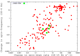
Figure 14: Plot of changes in the pulsar spin-down rate, $|\Delta\dot{\nu}|$, with spin-frequency due to glitches. The data points (red circles) are from the glitch table of the ATNF pulsar catalog. The data points for PSR 1833$-$1034 are denoted by squares.

PSR J1833$-$1034 also shows small but permanent changes in the slow-down rate at the glitches, and the typical fractional change of $\dot{\nu}$ is a few parts in $10^{-5}$ (Table 3). These small increases in $|\dot{\nu}|$ are thought to be due to the decrease in the effective moment of inertia of the crust, which includes all components of the star dynamically coupled to the crust. Decoupling of the superfluid moment of inertia during the unpinning state reduces the entire moment of inertia of the star. However, for the third and fourth glitches, we observe a decrease in $\dot{\nu}$. This sign change of $\dot{\nu}$ may imply a small increase in moment of inertia or a small decrease in spin-down torque at the time of the glitch.

We did not detect any exponential recovery or decay with time after the glitches in our data, for either the change in rotational frequency or its derivative. This may imply that there are only permanent changes in the rotational parameters when this pulsar glitches. However, there is also a possibility that this may be due to the fact that our sampling interval for the timing properties of this pulsar $-$ about a week to 10 days $-$ is somewhat coarser than what may be required to adequately sample the expected decay time-scale for such low amplitude glitches. For example, in case of the Crab pulsar, for glitches with an amplitude of the order of $\sim$ $10^{-8}$, the exponential decay time-scale is of $\sim$ 10 days (Wong et al., 2001). Such time scales would be hard to detect in our timing data, and would need a much more intensive campaign of observations.

For the general pulsar population it is found that glitches with small $\Delta\nu$ also have small changes in $|\dot{\nu}|$. This is shown in Fig. 14, using the database of the glitch table in the ATNF pulsar catalog , where a clear correlated trend can be seen. Our results of the glitch parameters for PSR J1833$-$1034 shows that this pulsar follows this trend quite well.

The level of strength and frequency of occurrence of glitches in a pulsar can be quantified by the glitch activity parameter, $A_{g}$, defined as the mean change in frequency per unit time owing to glitches (Lyne, 1999):

$$A_{g}=\frac{1}{T}\sum{\Delta\nu_{g}}$$ (7)

where $\sum{\Delta\nu_{g}}$ is the total increase of the frequency owing to all the glitches over an interval of $T$. Glitches are considered as events of angular momentum transfer from the superfluid interior to the crust of the neutron star. The same rate of angular momentum transfer can be achieved with frequent small glitches or occasional larger ones. The glitch activity parameter combines the amplitude and frequency of angular momentum loss due to glitches over the interval of $T$. $A_{g}$ is relatively insensitive to the additional discovery of smaller glitches as the quality of a given data set improves, and hence it can be used as a long-term indicator of glitch effects (Wong et al., 2001). We find $A_{g}$ $=$ $1.53\times 10^{-15}$ $s^{-2}$ for PSR J1833$-$1034.

Fig. 15 shows the range of known values of $A_{g}$, as well as its dependence on $|\dot{\nu}|$, for a collection of 32 pulsars. The data are mostly from literature (circles), except for a few points (triangles for B0611$+$22, B1853$+$01 and B0540$-$69) which are from unpublished results from observations at the Torun Radio Telescope by one of us (Wojciech Lewandowski). The literature references are as follow : Lyne et al. (2000) (B0833$-$45, B1325$-$43, B1535$-$56, B1641$-$45, B1727$-$33, B1736$-$29, B1758$-$23, B1800$-$21, B1823$-$13, B1830$-$08, B1859$+$07, B2224$+$65, B0355$+$54, B0525$+$21 and B1737$-$30), Wang et al. (2000) (B0833$-$45, B1046$-$58, J1105$-$6107, J1123$-$6259, B1338$-$62, B1610$-$50, B1706$-$44, B1727$-$47, B1758$-$23, B1757$-$24 and B1800$-$21,), Wong et al. (2001) (B0531$+$21), Hobbs et al. (2002) (J1806$-$2125), Urama (2002) (B1737$-$30), Weltevrede et al. (2011) (J1119$-$6127), Shabanova and Urama (2000) (B1822$-$09), Middleditch et al. (2006)) (J0537$-$6910), Livingstone et al. (2006) (J1846$-$0258). Though there is some scatter present, for a majority of pulsars there is an overall trend of increasing $A_{g}$ with increasing $|\dot{\nu}|$. This trend is mirrored in a plot of glitch activity versus characteristic age, as shown in Fig. 16 : glitch activity is higher for younger pulsars with characteristic age $\sim$ 10 kyr, and as the characteristic age increases, the activity falls off. These effects could be due to the fact that the flow of the angular momentum from the interior decreases with age (or increases with $|\dot{\nu}|$). There are a few pulsars with relatively higher values of $|\dot{\nu}|$ (or relatively smaller values of characteristic age) that have somewhat lower values of $A_{g}$, and hence lie off the main curve. Detailed investigation shows that these are a group of very young pulsars (i.e. low characteristic age), such as the Crab, PSR J1119$-$6127, PSR B1853$+$01, PSR J1846$-$0258 and PSR B0540$-$69. We find that our young pulsar J1833$-$1034 fits in very well with this group.

Glitches are thought to be caused by the release of stress built up during the regular spin-down of the pulsar. This stress on the pinned vortices in the superfluid interior gets released to the solid crust by a collective unpinning of many vortices. This unpinning process results in a sudden spin-up of the crust due to this discontinuous transfer of angular momentum from the interior, which in-turn is manifested in a change in observed pulsar frequency. Frequent, low amplitude glitches implies that the release of the built up stress happens in a more uniform and continuous manner than for pulsars which show few, large amplitude glitches. In other words, for the younger pulsars with larger slow-down rates, the flow of the angular momentum from the interior seems to be a smoother process. According to McKenna and Lyne (1990), the higher internal temperature associated with the younger neutron stars might prevent the build up of larger stresses. In such cases, stresses on the pinned vortices get relieved by thermal drift of the vortices from one pinning site to another in a gradual fashion, resulting in frequent low amplitude glitches. Hence such pulsars may constitute a distinct class of glitching pulsars: younger pulsars with lower glitch activity and higher internal temperatures. These relatively young pulsars may evolve towards the normal trend (i.e. towards right on Fig. 16) as they age.

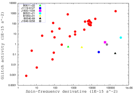
Figure 15: Plot of glitch activity parameter, $A_{g}$, versus the spin-down rate, $\dot{\nu}$, of pulsars. Circles are data points taken from literature and triangles are data points taken from Torun observations. The glitch activity of PSR 1833$-$1034 is denoted by the square.

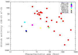
Figure 16: Plot of glitch activity parameter, $A_{g}$, versus characteristic age of pulsars. Circles are data points taken from literature and triangles are data points taken from Torun observations. The glitch activity of PSR 1833$-$1034 is denoted by the square.

5 Summary and future scope

In this paper we have presented results for four glitches detected in PSR J1833$-$1034, from 5.5 years of timing observations at the GMRT. These glitches show fractional change of the rotational frequency ranging from 1$\times 10^{-9}$ to 7$\times 10^{-9}$, with no evidence for any appreciable relaxation of the rotational frequency after the glitches. The fractional changes observed in the frequency derivative for this pulsar are of the order of $10^{-5}$. This pulsar appears to belong to a class of pulsars exhibiting fairly frequent occurrences of low amplitude glitches. We calculate the glitch activity parameter for PSR J1833$-$1034 to be $1.53\times 10^{-15}$ $s^{-2}$, which puts it in a special class of young pulsars like the Crab, and offset from the normal trend of glitch activity versus characteristic age (or spin frequency derivative) that a majority of the glitching pulsars follow. This could be related to the thermal history of young neutron stars.

The final timing solution obtained after modeling of the glitches provides reliable estimates of the second derivative of the spin-down model for PSR J1833$-$1034. The resulting braking index of 1.8569(6) is much less than the canonical value of 3, as also found for other young pulsars, supports the claim that pure dipole braking does not provide the full picture for pulsar spin-down.

With aid of the high time resolution and coherent dedispersion capabilities of the new GMRT Software Backend (Roy et al., 2010), we aim to search of giant pulse (GP) emission from this young pulsar. Though it is thought that most of the GP emitters are neutron stars with strong magnetic field at the light cylinder ($B_{LC}$ = $10^{4}$ to $10^{5}$ G) (Romani and Johnston, 2001), the detection of GPs in pulsars like J1752$+$2359 (Ershov and Kuzmin, 2006), B1112$+$50 (Ershov and Kuzmin, 2003) and B0031$-$07 (Kuzmin et al., 2004; Kuzmin and Ershov, 2004) reveals that GPs are also produced in pulsars with relatively low magnetic fields at the light cylinder. So even though the $B_{LC}$ of J1833-1034 is factor of 7 lower than the Crab, it can be worth searching for GPs using the coherent dedispersed output taken with the GSB.

6 Acknowledgments

The current work is based on 5.5 years of regular timing observations at the GMRT. We would like to thank all the staff members of the GMRT who are associated in maintaining and running of the telescope to make it available for the observations. We acknowledge the support of all the telescope operators who helped during these long extensive pulsar timing observations. The GMRT is run by the National Centre for Radio Astrophysics of the Tata Institute of Fundamental Research. We would like to thank Prof. Dipankar Bhattacharya for insightful discussions on the theory of glitches. We acknowledge the referee of this paper for his useful and constructive comments that helped to improve the quality of this paper significantly. Wojciech Lewandowski also acknowledges the support of the Polish Grant N N203 391934.

References

- Anderson and Itoh (1975) Anderson, P. W., Itoh, N., 1975, Nature, 256, 25.
- Arzoumanian et al. (1994) Arzoumanian, Z., Nice, D., J., Taylor, J., H., and Thorsett, S., E., 1994, ApJ, 422, 671.
- Camilo et al. (2006) Camilo, F, Ransom, S., M., Gaensler, B., M., Slane, P., O., Lorimer, D., R., Reynolds, J., Manchester, R., N., and Murray, S., S., 2006, A&A, 637, 456.
- Espinoza et al. (2011) Espinoza, C., M., Lyne, A., G., Stappers, B., W., and Kramer, M., 2011, arXiv:1102.1743v1.
- Ershov and Kuzmin (2003) Ershov, A., A., and Kuzmin, A., D., 2003, Pis’ma v AZh, 29, 111.
- Ershov and Kuzmin (2006) Ershov, A., A., and Kuzmin, A., D., 2006, Chin. J. Astron. Astrophys., 6, 30.
- Gupta et al. (2000) Gupta, Y., Gothoskar, P., B., Joshi, B., C., Vivekanand, M., Swain, R., Sirothia, S., and Bhat, N., D., R., 2000, in IAU Colloq. 177, Pulsar Astronomy, ed. Kramer, M., Wex, N., and Wielebinski, R., (ASP Conf. Ser. 202, San Francisco: ASP), 277.
- Gupta et al. (2005) Gupta, Y., Mitra, D., Green, D., A., and Achrayya, A., 2005, Current Science, 89, 853.
- Hobbs et al. (2002) Hobbs, G., Lyne, A., G., Joshi, B., C., Kramer, M., Stairs, I., H., Camilo, F., Manchester, R., N., D’Amico, N., Possenti, A., Kaspi, V., M., 2002, MNRAS, 333, L7.
- Hobbs et al. (2006) Hobbs, G., B., Edwards, R., T., Manchester, R., N., 2006, MNRAS, 369, 655.
- Hobbs et al. (2010) Hobbs, G., B., Lyne, A., G., and Kramer, M., 2010, MNRAS, 402, 1027.
- Janssen et al. (2006) Janssen, G., H. and Stappers, B., W., 2006 AA, 457, 611.
- Kaspi et al. (1994) Kaspi, V., M., Manchester, R., N., Siegman, B., Johnston, S. and Lyne, A., G., 1994, ApJ, 422, L83.
- Kuzmin and Ershov (2004) Kuzmin, A., D. and Ershov, A., A., 2004, AA, 427, 575.
- Kuzmin et al. (2004) Kuzmin, A., D., Ershov, A., A. and Losovsky, B., Ya, 2004, Pis’ma v AZh, 30, 285.
- Livingstone et al. (2005) Livingstone, M., A., Kaspi, V., M., Gavriil, F., P., 2005, ApJ, 633, 1095.
- Livingstone et al. (2006) Livingstone, M., A., Kaspi, V., M., Gotthelf, E., V. and Kuiper, L., 2006, ApJ, 647, 1286.
- Lyne et al. (1988) Lyne, A., G., Pritchard, R., S., Smith, F., G., 1988, MNRAS, 233, 667.
- Lyne (1999) Lyne, A., G., 1999, in Arzoumanian Z., van der Hooft F., van der Heuvel E. P. J. eds, Pulsar Timing, General Relativity and the Internal Structure of Neutron Stars, Koninklijke Nederlandse Akademie van Wetenschappen, Amsterdam, 141.
- Lyne et al. (1993) Lyne A., G., Pritchard R., S., Smith, F., G., 1993, MNRAS, 265, 1003.
- Lyne et al. (1995) Lyne, A., G., Pritchard, A., G., Shemar, S., L., 1995, ApA, 16, 179.
- Lyne et al. (2000) Lyne, A., G., Shemar, S., L., Smith, F., Graham, 2000, MNRAS, 315, 534.
- Manchester and Taylor (1977) Manchester, R., N., Taylor, J., H., 1977, Pulsars, San Francisco, CA (USA): W. H. Freeman.
- McKenna and Lyne (1990) McKenna, J., and Lyne, A., G., 1990, Nature, 343, 349.
- Middleditch et al. (2006) Middleditch, J., Marshall, F., E., Wang, Q., D., Gotthelf, E., V., and Zhang, W., 2006, ApJ, 652, 1531.
- Romani and Johnston (2001) Romani, R., W. and Johnston, S., 2001, ApJ, 557, L93.
- Roy et al. (2010) Roy J., Gupta Y., Ue-Li Pen, Peterson J.B., Kudale S., Kodilkar J., 2010, Experimental Astronomy, 28, 55.
- Shabanova and Urama (2000) Shabanova, T., V., Urama, J., O., 2000, AA, 354, 960.
- Shabanova (2009) Shabanova, T., V., 2009, ApJ, 700, 1009.
- Standish (1982) Standish, E., M., 1982, AA, 114, 297.
- Swarup et al. (1997) Swarup, G., Ananthakrishnan, S., Subrahmanya, C., R., Rao, A., P., Kulkarni, V., K., and Kapahi, V., K., 1997, in High Sensitivity Radio Astronomy, ed. Jackson, N., and Davis, R., J., (Cambridge: Cambridge University Press), 217.
- Urama (2002) Urama, J., O., 2002, MNRAS, 330, 58.
- Wang et al. (2000) Wang, N., Manchester, R. N., Pace, R. T., Bailes, M., Kaspi, V. M., Stappers, B. W., Lyne, A. G., 2000, MNRAS, 317, 843.
- Weltevrede et al. (2011) Weltevrede P., Johnston S., and Espinoza C., M., 2011, MNRAS, 411, 1917.
- Wong et al. (2001) Wong, T., Backer, D., C., Lyne, A., G., 2001, ApJ, 548, 447.
- Yuan et al. (2010) Yuan, J. P., Wang, N., Manchester, R. N., Liu, Z. Y., 2010, MNRAS, 404, 289.